Lifshitz

Avinash Dhar, Gautam Mandal and Partha Nag

Department of Theoretical Physics

Tata Institute of Fundamental Research,

Mumbai 400 005, INDIA

email: adhar, mandal, parthanag@theory.tifr.res.in

Abstract

We study renormalization group flows in the Lifshitz-like $N$-flavour four fermi model discussed in 0905.2928. In the large-$N$ limit, a nontrivial flow occurs in only one of all possible marginal couplings and one relevant coupling, which provides the scale for Lorentz invariance violations. We discuss in detail the phase diagram and RG flows in the space of couplings, which includes the Lifshitz fixed point, the free field fixed point and a new fixed point characterized by $z=1$ scaling and a violation of Lorentz invariance, which cannot be tuned away by adjusting a parameter. In the broken symmetry phase, the model flows from the $z=3$ Lifshitz-like fixed point in the ultraviolet to this new fixed point in the infrared. However, in a modified version of the present model, which has an effective ultraviolet cut-off much smaller than the Lorentz invariance violating scale, the infrared behaviour is governed by an approximately Lorentz invariant theory, similar to the low energy limit of the usual relativistic Nambu$-$Jona-Lasinio model. Such a modified model could be realized by a supersymmetric version of the present model.

1 Introduction

Recently, there has been considerable interest in field theories in which Lorentz invariance is explicitly violated by terms containing higher order spatial derivatives. The presence of these terms leads to softer ultraviolet behaviour while preserving unitarity (which is typically lost in the presence of Lorentz invariant higher derivative terms because of ghosts associated with higher time derivatives). At very high energies, these Lorentz invariance violating terms dominate, leading to Lifshitz-like anisotropic scaling symmetry (in the classical theory) in which time and space scale differently: $x\to x/a,t\to t/a^{z}$. The exponent $z$ characterizes the scaling symmetry.

Lifshitz-like field theories with anisotropic scaling have been used in condensed matter systems to describe quantum criticality [1]-[6]. Recently they have also been discussed in string theory in the context of possible applications of AdS/CFT duality [7]-[15] to condensed matter systems involving strongly interacting constituents. In a separate development, the idea that a relativistic theory at low energies may have a Lorentz non-invariant ultraviolet completion was suggested in [16]. This idea has been further explored in [17]-[25]. The suggestion that an ultraviolet completion of quantum gravity may be similarly formulated [26] has serious difficulties [27]-[33] because gravity elevates Lorentz invariance to a local gauge symmetry, which cannot be broken except by some kind of Higgs mechanism. In the present work we will focus only on non-gravitational theories.

Lifshitz-like field theories with Lorentz invariance violations (LIV) have also recently been discussed in the context of applications to particle physics [34, 35, 19, 25, 36, 37]. In [35, 19] it was argued that a $z=3$ Lifshitz-like ultraviolet completion of the Nambu$-$Jona-Lasinio (NJL) model [38] in $3+1$ space-time dimensions has the required properties to replace the Higgs sector of the electro-weak theory. The four-fermion coupling in this model is asymptotically free, leading to dynamical mass generation for the fermions and chiral symmetry breaking. In an appropriately gauged version, fluctuations of the magnitude of the fermion bilinear order parameter can be interpreted as the Higgs field. This model obviates the need for fine tuning at the expense of introducing LIV at high energies. The hope is that for a sufficiently large LIV scale, the low-energy theory could be consistent with experimental constraints on LIV. This may, however, require a new fine tuning of parameters [21].

The main purpose of this work is to analyze renormalization group (RG) flows in the model of [19] to understand in detail the possible emergence of Lorentz invariance at low energies. The analysis has been performed in the leading large-$N$ approximation. Our findings can be summarized as follows.

$\bullet$ At low energies, in the fermionic sector, the theory recovers approximate Lorentz invariance, violations being of order $E^{2}/\mu^{2}$, where $\mu$ is the energy scale associated with LIV. However, in the bosonic sector, in the broken chiral symmetry phase, the induced kinetic terms violate Lorentz invariance at ${\cal{O}}(1)$ level. The origin of these violations is simple to understand $-$ they arise from fermion modes with energies higher than $\mu$ propagating in a loop. These violations can be made small by imposing an effective cut-off on the theory and arranging $\mu$ to be much larger than the cut-off (see the last paragraph of Section 3).

$\bullet$ The RG flows reveal a new nontrivial fixed point, apart from the $z=3$ ultraviolet fixed point. The theory flows down from high energies to this fixed point at low energies. The above mentioned approximate Lorentz invariance in the fermionic sector and ${\cal{O}}(1)$ LIV in the bosonic sector are characteristic of this new fixed point. If one works with a fixed finite cut-off $\Lambda$, and sends the LIV scale $\mu$ much above $\Lambda$, the Lorentz violations become smaller and smaller, leading to an approximately Lorentz invariant theory which is identical to an effective theory derived from the NJL model at low energies, with a cut-off $\Lambda$.

The plan of the paper is as follows. In section 2 we deform the z=3 action with all possible marginal and relevant couplings (from the point of view of $z=3$ scaling) and study their effect on the vacuum solution. We find that only one of the three possible four-fermion (marginal) couplings has a nontrivial flow. Moreover, there is only one relevant coupling that affects the low energy physics, namely the coupling that determines the scale of LIV. This had already been remarked in [19], but section 2 provides a detailed justification for it. In section 3, we derive the effective action at a scale much smaller than the scale of LIV. We find that at low energies, in the broken symmetry phase, the kinetic terms induced by fermion loops for the massive scalar bound state of the fermions violate Lorentz invariance at ${\cal{O}}(1)$ level, which cannot be corrected by any fine-tuning of parameters. In section 4 we study the RG flow of the couplings and locate fixed points. We compare this fixed point structure with that in the relativistic NJL model. We end with some concluding remarks in section 5. Details of some of the calculations have been given in three Appendices.

2 The action and vacuum solutions

The model discussed in [19] consists of 2N species of fermions, $\psi_{ai}(t,\vec{x})$, where the index $a$ runs over the values $1,~{}2$ and the index $i$ runs from 1 to $N$. Each of these fermions is an $SU(2)$ spinor, where $SU(2)$ is the double cover of the spatial rotation group $SO(3)$. It is useful to view the index $a$ as denoting the two Weyl components of a Dirac fermion in a four dimensional theory with Lorentz invariance. The action we consider will have the following symmetries: a global $U(1)_{1}\times U(1)_{2}$ symmetry under which the fermions transform as

$$\psi_{ai}\to e^{i\alpha_{a}}\psi_{ai},\hskip 14.22636pta=1,2;$$ (1)

and a global $U(N)$ symmetry under which the fermions transform in the fundamental representation

$$\psi_{ai}\to U_{ij}\psi_{aj},\hskip 14.22636pti=1,...,N.$$ (2)

In addition to these symmetries, we will ensure that the action is invariant under the interchange $\psi_{1i}(t,\vec{x})\to\psi_{2i}(t,-\vec{x})$. This is the analogue of the parity operation in the relativistic Dirac theory.

A general action which is consistent with the above symmetries and contains all the relevant and marginal couplings is given by

$$\!\!\!S=\!\!\int\!\! \kern-18.0ptd^{3}\vec{x}\ dt\left[{\psi^{\dagger}}_{\!1i}\left\{i\partial_{t}-i\vec{\partial}.\vec{\sigma}\ \left(g_{0}(-i\vec{\partial})^{2}+g_{1}\right)-g_{2}\vec{\partial}^{2}\right\}\psi_{1i}\right.$$

$$\kern-18.0pt+{\psi^{\dagger}}_{\!2i}\left\{i\partial_{t}+i\vec{\partial}.\vec{\sigma}\ \left(g_{0}(-i\vec{\partial})^{2}+g_{1}\right)-g_{2}\vec{\partial}^{2}\right\}\psi_{2i}+g_{3}\left({\psi^{\dagger}}_{\!1i}\psi_{1i}+{\psi^{\dagger}}_{\!2i}\psi_{2i}\right)$$

$$\kern-18.0pt\left.+g_{4}^{2}\left\{\left({\psi^{\dagger}}_{\!\!1i}\psi_{1i}\right)^{2}+\left({\psi^{\dagger}}_{\!\!2i}\psi_{2i}\right)^{2}\right\}+g_{5}^{2}\left({\psi^{\dagger}}_{\!\!1i}\psi_{1i}{\psi^{\dagger}}_{2j}\psi_{2j}\right)+g^{2}\left({\psi^{\dagger}}_{\!\!1i}\psi_{2i}{\psi^{\dagger}}_{2j}\psi_{1j}\right)\right].$$

At high energies, this action has the scale invariance of a $z=3$ Lifshitz-like theory in which space and time have the dimensions $[x]=-1$ and $[t]=-3$. At low energies, the relevant term with coupling $g_{1}$ dominates, so one expects the model to flow down to an approximately Lorentz invariant theory at low energies. We will study the dynamics of this action in the large $N$ limit.

It is useful to employ the notation of Dirac matrices and rewrite the action (LABEL:relevant) in terms of the four-component spinor

$$\Psi_{i}=\left(\begin{array}[]{c}\psi_{1i}\\ \psi_{2i}\end{array}\right)$$ (6)

and its Weyl components $P_{L,R}\Psi_{i}={\Psi_{i}}_{L,R}=\psi_{1,2i}$. We will also use the Dirac gamma matrices

$$\gamma^{0}=\sigma_{1}\otimes{\bf 1},\quad\gamma^{i}=i\sigma_{2}\otimes\sigma_{i},\quad\gamma^{5}=i\gamma^{0}\gamma^{1}\gamma^{2}\gamma^{3}=\sigma_{3}\otimes{\bf 1},$$ (7)

where the $\sigma$’s are standard Pauli matrices satisfying $[\sigma_{i},\sigma_{j}]=i\epsilon_{ijk}\sigma_{k}$ and ${\bf 1}$ is the $2\times 2$ identity matrix. In terms of these matrices, the Weyl projection operators are given by $P_{L,R}=\frac{1}{2}(1\pm\gamma^{5})$. In this notation, the above action takes the form

$$S=\int \kern-18.0ptd^{3}\vec{x}\ dt\biggl{[}\bar{\Psi}_{i}\biggl{\{}\gamma^{0}\left(i\partial_{0}-g_{2}\vec{\partial}^{2}+g_{3}\right)+i\vec{\gamma}.\vec{\partial}\left(g_{1}-g_{0}\vec{\partial}^{2}\right)\biggr{\}}\Psi_{i}$$ (8)

$$\kern-18.0pt+g_{4}^{2}\biggl{\{}(\bar{\Psi}_{Li}\gamma^{0}\Psi_{Li})^{2}+(\bar{\Psi}_{Ri}\gamma^{0}\Psi_{Ri})^{2}\biggr{\}}+g_{5}^{2}(\bar{\Psi}_{Li}\gamma^{0}\Psi_{Li})(\bar{\Psi}_{Rj}\gamma^{0}\Psi_{Rj})$$

$$\kern-18.0pt+g^{2}(\bar{\Psi}_{Li}\Psi_{Rj})(\bar{\Psi}_{Rj}\Psi_{Li})\biggr{]},$$

As is usual for actions with four-fermion interactions, we now introduce auxiliary scalar fields to rewrite the above in the completely equivalent form of an action quadratic in fermions:

$$S=\int \kern-18.0ptd^{3}\vec{x}\ dt\biggl{[}\bar{\Psi}_{i}\biggl{\{}\gamma^{0}\left(i\partial_{0}-g_{2}\vec{\partial}^{2}+g_{3}\right)+i\vec{\gamma}.\vec{\partial}\left(g_{1}-g_{0}\vec{\partial}^{2}\right)+\left(\phi P_{L}+\phi^{\ast}P_{R}\right)$$ (9)

$$\kern-18.0pt+\gamma^{0}\left(\alpha P_{L}+\beta P_{R}\right)\biggr{\}}\Psi_{i}-\frac{\rho^{2}+\rho\eta}{g_{4}^{2}}-\frac{g_{4}^{2}\eta^{2}}{g_{5}^{2}}-\frac{|\phi|^{2}}{g^{2}}\biggr{]}.$$

Here $\rho$ and $\eta$ are real scalar fields and $\phi$ is a complex scalar field. We have also defined

$$2\rho+\eta\equiv\alpha,\qquad\frac{g_{5}^{2}}{g_{4}^{2}}\rho+2\frac{g_{4}^{2}}{g_{5}^{2}}\eta\equiv\beta.$$ (10)

The scalars are fermion bilinear composites, as can be easily derived from their equations of motion:

$$\rho=g_{4}^{2}(\bar{\Psi}_{Li}\gamma^{0}\Psi_{Li}),\qquad\eta=g_{5}^{2}(\bar{\Psi}_{Ri}\gamma^{0}\Psi_{Ri}),\qquad\phi=g^{2}(\bar{\Psi}_{Li}\Psi_{Ri}).$$ (11)

2.1 Vacuum solutions

Since the action (9) is quadratic in fermions, one can integrate these out to get an effective action for the scalar fields. For vacuum solutions, it is sufficient to consider only the homogeneous modes, $\rho_{0},~{}\eta_{0}$ and $\phi_{0}$, of the scalar fields. Moreover, without loss of generality, one may take $\phi_{0}$ to be real. In this case, the effective action for the scalars is given by

$$S_{eff}=-i \kern-18.0ptN\ {\rm Tr}\ln\biggl{\{}l_{0}\gamma^{0}-\vec{l}.\vec{\gamma}+\phi_{0}+\gamma^{0}(\alpha_{0}P_{L}+\beta_{0}P_{R})\biggr{\}}$$ (12)

$$\kern-18.0pt-\left(\frac{\rho_{0}^{2}+\rho_{0}\eta_{0}}{g_{4}^{2}}+\frac{g_{4}^{2}\eta_{0}^{2}}{g_{5}^{2}}+\frac{\phi_{0}^{2}}{g^{2}}\right)V,$$

where $V$ denotes the volume of space-time. Also, in the momentum space representation, we have

$$l_{0}(k_{0},\vec{k})=k_{0}+g_{2}k^{2}+g_{3},\qquad\vec{l}(\vec{k})=\vec{k}(g_{0}k^{2}+g_{1}),\qquad k=|\vec{k}|.$$ (13)

The equations of motion are obtained by varying this action with respect to $\rho_{0},~{}\eta_{0}$ and $\phi_{0}$. The calculation can be simplified by noticing that due to the “parity” symmetry $\Psi_{Li}(t,\vec{x})\to\Psi_{Ri}(t,-\vec{x})$, which we assume is unbroken, and the relations (11), the vacuum solutions $\rho_{0}$ and $\eta_{0}$ are related, i.e.

$$\rho_{0}/g_{4}^{2}=\eta_{0}/g_{5}^{2}.$$ (14)

Thus, there are really only two independent variables, $\rho_{0}$ and $\phi_{0}$ . Using this relation after varying (12) with respect to $\rho_{0},~{}\eta_{0}$ and $\phi_{0}$, the two independent equations of motion can be written as

$$\frac{\rho_{0}}{\lambda_{4}}=-2i\int\frac{d^{4}k}{(2\pi)^{4}}\frac{(l_{0}+\alpha_{0})}{(l_{0}+\alpha_{0})^{2}-\vec{l}^{2}-\phi_{0}^{2}},$$ (15)

$$\frac{1}{\lambda}=2i\int\frac{d^{4}k}{(2\pi)^{4}}\frac{1}{(l_{0}+\alpha_{0})^{2}-\vec{l}^{2}-\phi_{0}^{2}}.$$ (16)

where we have defined the ’t Hooft couplings,

$$g_{4,5}^{2}N\equiv\lambda_{4,5},\qquad g^{2}N\equiv\lambda,$$ (17)

and made use of the relation

$$\alpha_{0}=\beta_{0}=\left(2+\frac{\lambda_{5}}{\lambda_{4}}\right)\rho_{0},$$ (18)

which follows from equations (10) and (14). The equations (15) and (16) are exact in the usual large N limit in which the ’t Hooft couplings are held fixed.

Let us first consider equation (15). The momentum integral on the right hand side has a power divergence, so the dependence on $\alpha_{0}$ cannot be removed by shifting $k_{0}$. To do the integral, we need to introduce a regulator. We will use a simple cut-off regulator. Continuing to Euclidean momenta, we may then write

$$\tilde{\rho}_{0} = \frac{\lambda_{4}}{2\pi^{3}}\int_{0}^{M}dk\ k^{2}\int_{-M^{3}}^{M^{3}}dk_{0}\ \frac{k_{0}-g(k)}{\left(k_{0}-g(k)\right)^{2}+l^{2}+\phi_{0}^{2}}$$ (19)

$$= \frac{\lambda_{4}}{4\pi^{3}}\int_{0}^{M}dk\ k^{2}\ \ln\left\{\frac{l^{2}+\phi_{0}^{2}+\left(M^{3}-g(k)\right)^{2}}{l^{2}+\phi_{0}^{2}+\left(M^{3}+g(k)\right)^{2}}\right\},$$

where $l=|\vec{l}|=k|g_{0}k^{2}+g_{1}|$, $g(k)=(\tilde{g}_{2}k^{2}+\tilde{g}_{3}+\tilde{\alpha_{0}})$ and $\tilde{\rho}_{0}=i\rho_{0}$, $\tilde{g}_{2}=ig_{2}$ and $\tilde{g}_{3}=ig_{3}$ are Euclidean continuations of respectively $\rho_{0}$, $g_{2}$ and $g_{3}$.

In the limit of large $M$, the integral in (19) can be done by expanding both the numerator and denominator of the argument of the ‘ln’ function around $(M^{6}+g_{0}^{2}k^{6})$. Discarding terms that vanish as $M\rightarrow\infty$, we get

$$\rho_{0}=\frac{\lambda_{4}}{\pi^{3}}\biggl{\{}-M^{2}g_{2}I_{0}-(g_{3}+\alpha_{0})I_{1}+\left(2g_{0}g_{1}-g_{2}^{2}\right)g_{2}I_{2}+\frac{4}{3}g_{2}^{3}I_{3}\biggr{\}},$$ (20)

where the coefficients $I_{0},~{}I_{1},~{}I_{2}$ and $I_{3}$ are functions of $g_{0}$ only and are listed in Appendix 1. In writing the above, we have continued the various parameters and fields back to Minkowski signature. Now, using relation (18), the above equation can be solved for $\rho_{0}$:

$$\rho_{0}\left\{1+\left(2\lambda_{4}+\lambda_{5}\right)\frac{I_{1}}{\pi^{3}}\right\}$$

$$=\frac{\lambda_{4}}{\pi^{3}}\left\{-(g_{3}+M^{2}g_{2}I_{0}/I_{1})I_{1}+\left(2g_{0}g_{1}-g_{2}^{2}\right)g_{2}I_{2}+\frac{4}{3}g_{2}^{3}I_{3}\right\}.$$ (21)

Notice that $\rho_{0}$ vanishes if $g_{2}=g_{3}=0$. If $g_{2}=0$ but $g_{3}\neq 0$, then $\rho_{0}$ is nonzero, but we may take all the couplings appearing in the solution as fixed, independent of the cut-off. In case $g_{2}\neq 0$, then the right hand side of (21) diverges quadratically with the cut-off. However, this divergence can be removed by shifting $g_{3}$, i.e. we set $g_{3}=(g_{3}^{\prime}-M^{2}g_{2}I_{0}/I_{1})$, where $g_{3}^{\prime}$ is independent of the cut-off $M$. This determines $\rho_{0}$ in terms of the $M$-independent couplings $g_{2}$, $g_{3}^{\prime}$, $g_{4}$, etc.

The other vacuum parameter, $\phi_{0}$, is determined by equation (16). In this case, the integral over $k_{0}$ on the right hand side is convergent and the entire integral is only logarithmically divergent. So a shift of the integration variable $k_{0}$ is allowed. Doing this enables us to get rid of the couplings $g_{2},~{}g_{3},~{}g_{4},~{}g_{5}$ and $\rho_{0}$ from this gap equation. After a Euclidean continuation ($k_{0}=ik_{4}$) it then takes the form

$$\frac{1}{\lambda}=2\int\frac{d^{4}k}{(2\pi)^{4}}\frac{1}{(k_{4}^{2}+l^{2}(k)+\phi_{0}^{2})}.$$ (22)

As discussed in [19], this equation signals the breaking of the global $U(1)_{1}\times U(1)_{2}$ “chiral” symmetry (1) down to $U(1)$. It also requires that the coupling $\lambda$ have a nontrivial RG flow, which depends on the couplings $g_{0}$ and $g_{1}$. We will analyze this flow in detail in section 4.

We end this section with the following comment. It should be clear from the above discussion that in the present model all the interesting dynamics arises from the NJL type of four fermi interaction (conjugate to the ’t Hooft coupling $\lambda$) and its RG flow is decoupled from the dynamics of all the other marginal couplings. Therefore, for calculational simplicity, in the rest of the paper we will set the marginal couplings $g_{4}$ and $g_{5}$ to zero. We will also set $g_{2}=g_{3}=0$ since these couplings also do not affect the RG flow of $\lambda$.

3 Low energy effective action

Setting $g_{2}=g_{3}=g_{4}=g_{5}=0$ in (8) as discussed above, and going over to the bosonic variable $\phi(x)$ as in (9), we get the action

$$S=\int d^{4}x\biggl{[} \kern-18.0pt\bar{\Psi}_{i}\biggl{\{}i\gamma^{0}\partial_{0}+i\vec{\gamma}.\vec{\partial}\left(g_{1}-g_{0}\vec{\partial}^{2}\right)+(\phi P_{L}+\phi^{*}P_{R})\biggr{\}}\Psi_{i}-\frac{N}{\lambda}|\phi|^{2}\biggr{]}.$$

We are interested in the low energy effective action for this system in the phase in which the symmetry (1) is broken. To derive the low energy action, we substitute in the above $\phi(x)=(\phi_{0}+\frac{\sigma(x)}{\sqrt{N}})e^{i\frac{\theta(x)}{\sqrt{N}}}$, where $\phi_{0}$ is the vacuum solution and $\sigma(x)$ and $\theta(x)$ are respectively the magnitude and phase of the fluctuation of $\phi(x)$ around the vacuum. We get,

$$S=\int d^{4}x\biggl{[} \kern-18.0pt\bar{\Psi}_{i}\biggl{\{}i\gamma^{0}\partial_{0}+i\vec{\gamma}.\vec{\partial}\left(g_{1}-g_{0}\vec{\partial}^{2}\right)+\biggl{(}\phi_{0}+\frac{\sigma}{\sqrt{N}}\biggr{)}\biggl{(}P_{L}e^{i\frac{\theta}{\sqrt{N}}}+P_{R}e^{-i\frac{\theta}{\sqrt{N}}}\biggr{)}\biggr{\}}\Psi_{i}$$ (24)

$$\kern-18.0pt-\frac{1}{\lambda}\sigma^{2}-\frac{2\sqrt{N}}{\lambda}\phi_{0}\sigma-\frac{N}{\lambda}\phi_{0}^{2}\biggr{]}.$$

The phase $\theta$ is the Goldstone mode. It can be “rotated” away from the Yukawa-type coupling by making the change of variables $\Psi_{iL}\rightarrow e^{-i\frac{\theta}{2\sqrt{N}}}\Psi_{iL}$ and $\Psi_{iR}\rightarrow e^{i\frac{\theta}{2\sqrt{N}}}\Psi_{iR}$. Its derivatives will, however, now appear from the fermion kinetic terms. After this change of variables, the action takes the form

$$S=\int d^{4}x\biggl{[} \kern-18.0pt\bar{\Psi}_{i}\biggl{\{}i\gamma^{0}\partial_{0}+i\vec{\gamma}.\vec{\partial}\left(g_{1}-g_{0}\vec{\partial}^{2}\right)+\phi_{0}+\frac{\sigma}{\sqrt{N}}\biggr{\}}\Psi_{i}+{\cal O}(\bar{\Psi}\partial\theta\Psi)$$ (25)

$$\kern-18.0pt-\frac{1}{\lambda}\sigma^{2}-\frac{2\sqrt{N}}{\lambda}\phi_{0}\sigma-\frac{N}{\lambda}\phi_{0}^{2}\biggr{]},$$

where ${\cal O}(\bar{\Psi}\partial\theta\Psi)$ indicates terms involving derivatives of the Goldstone mode $\theta$. In the following we will ignore these terms and retain only the mode $\sigma$. There is no basic difficulty in retaining $\theta$ also, but this is not essential for describing the RG flow of $\lambda$ and LIV properties of the low energy action.

To proceed further, it is convenient to rewrite the action (25) in momentum space. We have

$$S= \kern-18.0pt\int\frac{d^{4}k}{(2\pi)^{4}}\int\frac{d^{4}q}{(2\pi)^{4}}\bar{\Psi}_{i}(k)\biggl{\{}\left(\gamma^{0}k_{0}-\vec{\gamma}.\vec{l}(\vec{k})+\phi_{0}\right)(2\pi)^{4}\delta^{4}(k-q)+\frac{1}{\sqrt{N}}\sigma(k-q)\biggr{\}}\Psi_{i}(q)$$ (26)

$$\kern-18.0pt-\int\frac{d^{4}k}{(2\pi)^{4}}\frac{1}{\lambda}\ |\sigma(k)|^{2}-\frac{2\sqrt{N}}{\lambda}\phi_{0}\sigma(k=0)-\frac{VN}{\lambda}\phi_{0}^{2},$$

where $V$ denotes the volume of space-time and $\vec{l}(\vec{k})$ is given by (13). As discussed in the next section, although this action depends on the two parameters $g_{0}$ and $g_{1}$, the physics described by it actually depend on only a particular combination of these, namely

$$\mu=|g_{1}^{3}/g_{0}|^{\frac{1}{2}}.$$ (27)

$\mu$ has the dimensions of energy. As discussed below, its significance is that it is the energy scale at which Lorentz violations become important. The action (26) can, in fact, be explicitly written in terms of this combination. However, two different versions of the action are needed to cover the entire line of real values of $\mu$, from zero to infinity. In the form (26), the action is valid for all values, but at the expense of having a redundant variable. We will discuss this issue further in the next section after we have obtained the low energy action.

The action at low energies is obtained by integrating out high energy modes from this action. To carry out this procedure, we will need to regularize divergences in loop momentum integrals, which we will do by using a cut-off that scales like energy. However, the way in which the cut-off is imposed needs to be chosen carefully, because an arbitrarily chosen cut-off procedure (in a theory with LIV) might preclude the possibility of an approximate restoration of Lorentz invariance at low energies. We choose to impose a cut-off on the expression $(k_{4}^{2}+l^{2}(k))$, where $k_{4}=-ik_{0}$ is the Euclidean continuation of energy. To understand why it is natural to adopt this cut-off procedure, recall the definition of $l(k)=|\vec{l}(\vec{k})|=k|g_{0}k^{2}+g_{1}|$, given in (13). Now, for $g_{1}\neq 0$, we can completely scale it out of this expression by the scaling $k\rightarrow k/|g_{1}|$. This gives $l\rightarrow k|\epsilon\mu^{-2}k^{2}+1|$, where $\epsilon=\pm 1$ is the relative sign of $g_{0}$ with respect to $g_{1}$. For $k<<\mu$, $(k_{4}^{2}+l^{2}(k))$ can be well approximated by the $SO(4)$-invariant form $(k_{4}^{2}+k^{2})$. Thus, the proposed cut-off is naturally consistent with the possibility of Lorentz symmetry restoration at low energies.

In the following we will use the notation $\int[d^{4}k]_{E\rightarrow\Lambda}$ to indicate that the integral over Euclidean momenta is restricted to the region $E^{2}\leq(k_{4}^{2}+l^{2}(k))\leq\Lambda^{2}$, i.e.

$$\int[d^{4}k]_{E\rightarrow\Lambda}\ \cdots\ \equiv$$

$$~{}~{}~{}~{}~{}~{}~{}\int d^{4}k\ \theta\left(\Lambda^{2}-(k_{4}^{2}+l^{2}(k))\right)\theta\left((k_{4}^{2}+l^{2}(k))-E^{2}\right)\ \cdots,$$ (28)

where the $\theta$ is the usual step function. Note that both $\Lambda$ and $E$ have dimensions of energy. For the special case of $E=0$, it will be convenient to use the more compact notation $\int[d^{4}k]_{\Lambda}$.

Let us now integrate out from (26) all the modes between $(k_{4}^{2}+l^{2}(k))=\Lambda^{2}$ and $(k_{4}^{2}+l^{2}(k))=E^{2}$, where $\Lambda$ is the cut-off and $E<\Lambda$. The action with the lower energy cut-off $E$ is given by

$$S\kern-10.0pt = \kern-5.0pt\int\frac{[d^{4}k]_{E}}{(2\pi)^{4}}\kern-5.0pt\int\frac{[d^{4}q]_{E}}{(2\pi)^{4}}\ \bar{\Psi}_{i}(k)\biggl{\{}\kern-2.0pt(2\pi)^{4}\biggl{(}k_{0}\gamma^{0}-\vec{l}(\vec{k}).\vec{\gamma}+\phi_{0}\biggr{)}\delta^{4}(k-q)+\frac{\sigma(k-q)}{\sqrt{N}}\kern-2.0pt\biggr{\}}\Psi_{i}(q)$$ (29)

$$-\int\frac{[d^{4}k]_{E}}{(2\pi)^{4}}\left(C_{0}+C_{1}k_{0}^{2}-C_{2}k^{2}\right)|\sigma(k)|^{2}-2C_{3}\sqrt{N}\phi_{0}\sigma(k=0)-\frac{\phi_{0}^{2}NV}{\lambda}$$

$$+{\rm~{}classical~{}part}.$$

Details of the calculation leading to (29) as well as the calculations of the coefficients $C_{n}~{}(n=0,1,2,3)$ have been given in Appendix B. We have retained terms only up to ${\cal O}(1)$ in large $N$ and up to two derivatives of $\sigma(x)$. The “classical part” refers to the contribution which comes from the action evaluated on the classical solution.

Notice that even though the scalar field started out as an auxiliary field, it has now developed kinetic terms. As can be seen from equations (58)-(60), these terms imply a maximum attainable velocity at low energies for the $\sigma$ particle, which is given by

$$c_{\sigma}^{2}=\frac{C_{2}}{C_{1}}=c_{\psi}^{2}\ \frac{\bar{C_{2}}}{\bar{C_{1}}},$$ (30)

where $c_{\psi}=|g_{1}|$ is the maximum attainable velocity of the fermions at low energies. The quantities ${\bar{C}_{1,2}}$ have been defined in (60). In general $c_{\sigma}\neq c_{\psi}$, leading to LIV at low energies. As a check on our calculations, it is not difficult to see that for $g_{0}=0$, $c_{\sigma}=|g_{1}|$. Thus, we recover properties of the usual relativistic NJL model in the appropriate limit. Note that for $g_{0}\neq 0$, the model is renormalizable since the momentum integrals involved in the computation of $C_{1,2}$ are finite in the limit $\Lambda\rightarrow\infty$. However, for $g_{0}=0$, a finite $\Lambda$ is essential since in this usual, nonrenormalizable, relativistic NJL case the momentum integrals diverge.

What is the extent of the LIV at low energies? It follows from the above discussion that the magnitude of LIV depends on the deviation of the ratio $c_{\sigma}/c_{\psi}$ from unity. From equations (58)-(60) in Appendix B, we see that this quantity depends on the various energy scales only through the dimensionless ratios

$$\mu_{R}\equiv\mu/E,\qquad\bar{\mu}\equiv\mu/\Lambda.$$ (31)

In Figure 1 we have plotted $c_{\sigma}/c_{\psi}$ as a function of $\mu_{R}^{-1}$ for different values of $\bar{\mu}$.

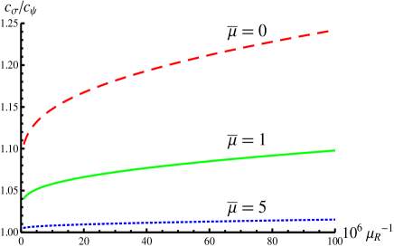
Figure 1: The variation of the ratio $c_{\sigma}/c_{\psi}$, or equivalently $({\bar{C}_{2}}/{\bar{C}_{1}})^{1/2}$, cf. (30), with $\mu_{R}^{-1}$ for different values of $\bar{\mu}$. This ratio measures Lorentz invariance violations. The dashed curve corresponds to $\bar{\mu}=0$. The other two cases have $\bar{\mu}=1$ and $5$. We have used $\phi_{0}/\mu=10^{-3}$.

In these plots, we have chosen the relative sign of $g_{0}$ and $g_{1}$ to be positive, i.e. $\epsilon=+1$. The dashed line in Figure 1 corresponds to case with $\bar{\mu}=0$, i.e. the case in which the cut-off $\Lambda$ is infinite. We see that even at very large values of $\mu_{R}$ there is violation of Lorentz invariance at ${\cal O}(1)$ level. The origin of these LIVs becomes clear from the other two lines in Figure 1. The full line corresponds to the case with $\bar{\mu}=1$ and for the dotted line $\bar{\mu}=5$. We see that the LIVs are dramatically reduced in these cases, being smaller for larger value of $\bar{\mu}$. Clearly, fermion modes with energy larger than $\mu$ propagating in the loop (Eq. (52)) make Lorentz violating contributions to $C_{1,2}$ at ${\cal O}(1)$ level. These modes can be removed from the loop by imposing a cut-off which is smaller than the LIV scale, i.e. for $\bar{\mu}>1$. For smaller cut-off, the effect should be better. This is precisely what we see in the calculations shown in Figure 1.

It should be emphasized that the ${\cal O}(1)$ violations of Lorentz invariance at low energies that we have found in the bosonic sector of the present model cannot be tuned away by adjusting any parameter. This makes (an appropriately gauged version of) the present model an unsuitable candidate for an alternative solution to the hierarchy problem. A way out could be provided by a supersymmetric extension of the model. If supersymmetry is broken at a scale $M_{s}$ much smaller than the Lorentz invariance violating scale $\mu$, then a cancellation with bosonic partners would remove the Lorentz violating contributions from fermionic modes with energy larger than $M_{s}$ propagating in the loop. This essentially means that the role of the cut-off $\Lambda$ would then be played by $M_{s}$. The residual low energy LIV would then be controlled by $M_{s}^{2}/\mu^{2}$, which can be made small by tuning the scale at which supersymmetry is broken. Existing constraints on LIV coming from bounds on the maximum attainable velocity of various particles ($\delta c<10^{-24}$) [39]-[42] implies $M_{s}/\mu<10^{-12}$. For $\mu\sim 10^{17}$GeV, this means that supersymmetry can be broken at a much higher scale, $M_{s}\sim 100$ TeV, than in the currently popular scenarios. The present scenario might become a serious possibility, should LHC see a composite Higgs but no supersymmetry.

4 RG flows and fixed points

Classically, at high enough energies (where all masses can be ignored), the action in (25) has the scaling symmetry under which $x^{0}\rightarrow x^{0}/a^{3},\ \vec{x}\rightarrow\vec{x}/a,\ \Psi\rightarrow a^{3/2}\Psi,\ \sigma\rightarrow a^{3}\sigma$, where $a$ is the parameter of scaling transformation. This is the $z=3$ Lifshitz-like fixed point. For $g_{0}=0$, classically the free fermi theory has the scaling symmetry $x^{0}\rightarrow x^{0}/a,\ \vec{x}\rightarrow\vec{x}/a,\ \Psi\rightarrow a^{3/2}\Psi$. This is the familiar Lorentz invariant case, which can be described in the above language as a $z=1$ fixed point. At energies much smaller than the scale $\mu$, Lorentz violations are small even for $z=3$, and so classically one recovers an approximately Lorentz invariant theory at low energies. In the following, we will study RG flow in the quantum theory from the $z=3$ fixed point in the ultraviolet to find out what theory it flows to in the infrared.

4.1 Determination of renormalized parameters

In order to study the flow from high to low energies, we need to find out how the various couplings get renormalized. The starting point in the determination of the renormalization of the couplings in action (26), in the leading large $N$ approximation, is the low energy action (29). To implement the Wilson RG procedure, we need to rescale the cut-off $E$ in (29) back to the original cut-off $\Lambda$. As discussed above equation (27), our cut-off procedure imposes the restriction $(k_{4}^{2}+l^{2}(k))\leq\Lambda^{2}$ on Euclidean space momentum integrals. Writing $E=b\Lambda$, we see that the cut-off $E$ on the low energy action (29) can be rescaled to $\Lambda$ by the scale transformations (change of variables) $k_{4}\rightarrow bk_{4},\ k\rightarrow ak$, followed by the scalings of the couplings

$$a^{3}g_{0}=bg_{0}^{\prime},\qquad ag_{1}=bg_{1}^{\prime}.$$ (32)

These give the renormalized couplings and RG flow in the free fermion theory. Notice that the scaling parameter, $b$, for the energy is, a priori, unrelated to the scaling parameter, $a$, for the momenta. The $z=3$ fixed point behaviour corresponds to choosing $a=b^{1/3}$, and then the couplings scale as $g_{0}^{\prime}=g_{0}$ and $g_{1}^{\prime}=b^{-2/3}g_{1}$. Since in this case $g_{0}$ is invariant under the RG flow, we can set it to unity by scaling $k\rightarrow|g_{0}|^{-1/3}k$, leaving only one independent coupling, namely $g_{1}$. Choosing $a=b$ instead, one gets $g_{0}^{\prime}=b^{2/3}g_{0}$ and $g_{1}^{\prime}=g_{1}$, which are the scalings appropriate for a $z=1$ fixed point. In this case, $g_{1}$ is invariant under the RG flow and so we can scale it away by $k\rightarrow k/|g_{1}|$. Once again we are left with only one independent coupling.

The two fixed point behaviours discussed above can be treated together by setting $a=b^{1/z}$ where $z=3$ or $1$ . Then, using the cut-off $\Lambda$ to define the dimensionless renormalized couplings, we get

$$g_{0R}\equiv\Lambda^{\frac{3}{z}-1}g_{0}^{\prime}=E^{\frac{3}{z}-1}g_{0},\qquad g_{1R}\equiv\Lambda^{\frac{1}{z}-1}g_{1}^{\prime}=E^{\frac{1}{z}-1}g_{1}.$$ (33)

They satisfy the RG equations

$$\dot{g}_{0R}=-\left(\frac{3}{z}-1\right)g_{0R},\qquad\dot{g}_{1R}=-\left(\frac{1}{z}-1\right)g_{1R},$$ (34)

where a dot denotes a derivative with respect to ($-{\rm ln}E)$ . Using these two couplings, we can define the renormalized version of (27):

$$|g_{1R}^{3}/g_{0R}|^{\frac{1}{2}}=\mu/E=\mu_{R}.$$ (35)

This is precisely the quantity defined in (31).

In the leading large-$N$ approximation, the free field renormalization (34) is not affected by the Yukawa coupling. However, the ’t Hooft coupling $\lambda$ does receive quantum corrections. Its renormalization can be deduced from the term proportional to $C_{0}$ in the low energy action (29). Scaling the cut-off $E$ back to $\Lambda$ in (29) and using the expression for $C_{0}$ given in (57), we get

$$\frac{1}{\lambda^{\prime}}=\frac{b}{a^{3}}\biggl{\{}\frac{1}{\lambda}-2\int\frac{[d^{4}k]_{E\rightarrow\Lambda}}{(2\pi)^{4}}\ \frac{k_{4}^{2}+l^{2}(k)-\phi_{0}^{2}}{(k_{4}^{2}+l^{2}(k)+\phi_{0}^{2})^{2}}\biggr{\}},$$ (36)

Now, using $(\int[d^{4}k]_{E\rightarrow\Lambda}\ \cdots)=(\int[d^{4}k]_{\Lambda}\ \cdots)-(\int[d^{4}k]_{E}\ \cdots)$ and substituting $a=b^{1/z}$, we can simplify this equation to get

$$\frac{1}{\lambda^{\prime}}=b^{1-\frac{3}{z}}\biggl{\{}\xi+2\int\frac{[d^{4}k]_{E}}{(2\pi)^{4}}\ \frac{k_{4}^{2}+l^{2}(k)-\phi_{0}^{2}}{(k_{4}^{2}+l^{2}(k)+\phi_{0}^{2})^{2}}\biggr{\}},$$ (37)

where

$$\xi\equiv\frac{1}{\lambda}-2\int\frac{[d^{4}k]_{\Lambda}}{(2\pi)^{4}}\ \frac{k_{4}^{2}+l^{2}(k)-\phi_{0}^{2}}{(k_{4}^{2}+l^{2}(k)+\phi_{0}^{2})^{2}}.$$ (38)

So, for the dimensionless renormalized coupling, $\lambda_{R}\equiv\Lambda^{\frac{3}{z}-1}\lambda^{\prime}$, we get

$$\frac{1}{\lambda_{R}}=\frac{1}{E^{\frac{3}{z}-1}}\biggl{\{}\xi+2\int\frac{[d^{4}k]_{E}}{(2\pi)^{4}}\ \frac{k_{4}^{2}+l^{2}(k)-\phi_{0}^{2}}{(k_{4}^{2}+l^{2}(k)+\phi_{0}^{2})^{2}}\biggr{\}}.$$ (39)

This leads to the RG equation

$$\dot{\lambda}_{R}=-\left(\frac{3}{z}-1\right)\lambda_{R}+\frac{(1-\phi_{R}^{2})}{(1+\phi_{R}^{2})^{2}}\ \frac{\lambda_{R}^{2}}{\pi^{3}|g_{0R}|}\int_{0}^{h_{0}}ds\ \frac{s^{2}}{\sqrt{1-s^{2}(\epsilon s^{2}+\mu_{R}^{\frac{2}{3}})^{2}}}$$ (40)

where $\epsilon=\pm 1$ is the relative sign of $g_{0}$ and $g_{1}$, $\phi_{R}\equiv\phi_{0}/E$ is the dimensionless renormalized coupling corresponding to the vev (with the RG equation $\dot{\phi}_{R}=\phi_{R}$) and

$$h_{0}=\left(\frac{1}{2}+\sqrt{\frac{1}{4}+\frac{\mu_{R}^{2}}{27}}\right)^{\frac{1}{3}}-\frac{\mu_{R}^{\frac{2}{3}}}{3}\left(\frac{1}{2}+\sqrt{\frac{1}{4}+\frac{\mu_{R}^{2}}{27}}\right)^{-\frac{1}{3}}$$ (41)

Note that the form in which the right-hand side of (40) has been written is inappropriate for the special case $g_{0R}=0$. In this case one must use the alternative, but entirely equivalent, form:

$$\dot{\lambda}_{R}=-\left(\frac{3}{z}-1\right)\lambda_{R}+\frac{(1-\phi_{R}^{2})}{(1+\phi_{R}^{2})^{2}}\ \frac{\lambda_{R}^{2}}{\pi^{3}|g_{1R}|^{3}}\int_{0}^{h_{1}}ds\ \frac{s^{2}}{\sqrt{1-s^{2}(\epsilon\mu_{R}^{-2}s^{2}+1)^{2}}},$$ (42)

where $h_{1}=h_{0}\mu_{R}^{\frac{2}{3}}$. It is easy to see that $h_{1}\rightarrow 1$ as $\mu_{R}\rightarrow\infty$.

4.2 The renormalized action

In terms of the dimensionless renormalized couplings, the low energy action (29) can be written as

$$S = \int\frac{[d^{4}k]_{\Lambda}}{(2\pi)^{4}}\int\frac{[d^{4}q]_{\Lambda}}{(2\pi)^{4}}\ \bar{\Psi}_{iR}(k)\biggl{\{}(2\pi)^{4}\Lambda\biggl{(}\tilde{k}_{0}\gamma^{0}-\vec{l_{R}}(\vec{\tilde{k}}).\vec{\gamma}+\phi_{R}\biggr{)}\delta^{4}(k-q)$$ (43)

$$+\frac{1}{\sqrt{N}}\sigma_{R}(k-q)\biggr{\}}\Psi_{iR}(q)-\Lambda^{\frac{3}{z}-1}\int\frac{[d^{4}k]_{\Lambda}}{(2\pi)^{4}}\left(\frac{1}{\lambda_{R}}+C_{1R}\tilde{k}_{0}^{2}-C_{2R}\tilde{k}^{2}\right)|\sigma_{R}(k)|^{2}$$

$$-2\frac{\Lambda^{\frac{3}{z}}}{\lambda_{R}}\sqrt{N}\phi_{R}\sigma_{R}(k=0)\ +\ \text{classical part},$$

where $\vec{l_{R}}(\vec{\tilde{k}})=\vec{\tilde{k}}(g_{0R}\tilde{k}^{2}+g_{1R}),\ \tilde{k}_{0}=k_{0}/\Lambda,\ \tilde{k}=k\Lambda^{-\frac{1}{z}}$. Moreover, the renormalized fields are related to the bare fields by $\Psi_{iR}=b^{\frac{3}{2z}+1}\Psi_{i},\ \sigma_{R}=b^{\frac{3}{z}}\sigma$. The coefficients $C_{1,2R}$ are related to $C_{1,2}$ and have been defined in (62).

This action seems to depend separately on the two couplings $g_{0R},\ g_{1R}$, but actually the physics described by it depends only on the combination $\mu_{R}$, (35). To see this more explicitly, let us make the change of variables $\tilde{k}\rightarrow\tilde{k}/|g_{1R}|,\ \Psi_{iR}\rightarrow|g_{1R}|^{\frac{3}{2}}\Psi_{iR},\ \sigma_{R}\rightarrow|g_{1R}|^{3}\sigma_{R},\ \lambda_{R}\rightarrow\lambda_{1}=\lambda_{R}/|g_{1R}|^{3}$. After this change of variables, the action takes the form

$$S = \int\frac{[d^{4}k]_{\Lambda}}{(2\pi)^{4}}\int\frac{[d^{4}q]_{\Lambda}}{(2\pi)^{4}}\ \bar{\Psi}_{iR}(k)\biggl{\{}(2\pi)^{4}\Lambda\biggl{(}\tilde{k}_{0}\gamma^{0}-\vec{\tilde{l}}_{R}(\vec{\tilde{k}}).\vec{\gamma}+\phi_{R}\biggr{)}\delta^{4}(k-q)$$ (44)

$$+\frac{1}{\sqrt{N}}\sigma_{R}(k-q)\biggr{\}}\Psi_{iR}(q)-\Lambda^{\frac{3}{z}-1}\int\frac{[d^{4}k]_{\Lambda}}{(2\pi)^{4}}\left(\frac{1}{\lambda_{1}}+\bar{C}_{1}\tilde{k}_{0}^{2}-\bar{C}_{2}\tilde{k}^{2}\right)|\sigma_{R}(k)|^{2}$$

$$-2\frac{\Lambda^{\frac{3}{z}}}{\lambda_{1}}\sqrt{N}\phi_{R}\sigma_{R}(k=0)\ +\ \text{classical part},$$

where $\vec{\tilde{l}}_{R}(\vec{\tilde{k}})=\vec{\tilde{k}}(\epsilon\tilde{k}^{2}/\mu_{R}^{2}+1)$ and $\bar{C}_{1,2}$ are given by (61). This form of the action makes it explicit that physics depends only on the combination $\mu_{R}$ since any separate dependence on $g_{0R},\ g_{1R}$ has now disappeared.

The form (44) of the low energy action is not suitable for small values of $\mu_{R}$ (equivalently for small values of $g_{1R}$ or large values of $g_{0R}$). In this case, a more suitable change of variables in the action (43) is $\tilde{k}\rightarrow\tilde{k}|g_{0R}|^{-\frac{1}{3}},\ \Psi_{iR}\rightarrow|g_{0R}|^{\frac{1}{2}}\Psi_{iR},\ \sigma_{R}\rightarrow|g_{0R}|\sigma_{R},\ \lambda_{R}\rightarrow\lambda_{3}=\lambda_{R}/|g_{0R}|$. After this change of variables, the action takes the form

$$S = \int\frac{[d^{4}k]_{\Lambda}}{(2\pi)^{4}}\int\frac{[d^{4}q]_{\Lambda}}{(2\pi)^{4}}\ \bar{\Psi}_{iR}(k)\biggl{\{}(2\pi)^{4}\Lambda\biggl{(}\tilde{k}_{0}\gamma^{0}-\vec{\tilde{l}}_{R}^{\prime}(\vec{\tilde{k}}).\vec{\gamma}+\phi_{R}\biggr{)}\delta^{4}(k-q)$$ (45)

$$+\frac{1}{\sqrt{N}}\sigma_{R}(k-q)\biggr{\}}\Psi_{iR}(q)-\Lambda^{\frac{3}{z}-1}\int\frac{[d^{4}k]_{\Lambda}}{(2\pi)^{4}}\left(\frac{1}{\lambda_{3}}+C_{1}^{\prime}\tilde{k}_{0}^{2}-C_{2}^{\prime}\tilde{k}^{2}\right)|\sigma_{R}(k)|^{2}$$

$$-2\frac{\Lambda^{\frac{3}{z}}}{\lambda_{3}}\sqrt{N}\phi_{R}\sigma_{R}(k=0)\ +\ \text{classical part},$$

where $\vec{\tilde{l}}_{R}^{\prime}(\vec{\tilde{k}})=\vec{\tilde{k}}(\epsilon\tilde{k}^{2}+\mu_{R}^{\frac{2}{3}})$ and $C_{1}^{\prime}=\bar{C}_{1}\mu_{R}^{-2},\ C_{2}^{\prime}=\bar{C}_{2}\mu_{R}^{-2/3}$. It can be shown that $C_{1,2}^{\prime}$ have a finite limit as $\mu_{R}\rightarrow 0$; see equations (60)-(65). This form of the low energy action is now suitable for small values of $\mu_{R}$.

We have thus found two equally valid descriptions of the physics of the 4-fermi theory. One is that given by the action in (43), which is valid for all the values of the renormalized coupling $\mu_{R}$. However, in this form the action depends on two couplings, $g_{0R}$ and $g_{1R}$. In the form (44) and (45), the low energy action depends only on the combination $\mu_{R}$ of these, but two different descriptions are needed to cover the entire range of possible values of $\mu_{R}$.

4.3 Fixed points

As we have argued above, the relevant renormalized coupling constants in the low energy theory are $\lambda_{1}=\lambda_{R}/|g_{1R}|^{3}$ and $\lambda_{3}=\lambda_{R}/|g_{0R}|$, with $\lambda_{3}=\mu_{R}^{2}\lambda_{1}$. The RG equations for these can be obtained from equations (40) and (42) using (34). We get

$$\dot{\lambda}_{3} = \frac{(1-\phi_{R}^{2})}{(1+\phi_{R}^{2})^{2}}\ \frac{\lambda_{3}^{2}}{\pi^{3}}\int_{0}^{h_{0}}ds\ \frac{s^{2}}{\sqrt{1-s^{2}(\epsilon s^{2}+\mu_{R}^{\frac{2}{3}})^{2}}}.$$ (46)

$$\dot{\lambda}_{1} = -2\lambda_{1}+\frac{(1-\phi_{R}^{2})}{(1+\phi_{R}^{2})^{2}}\ \frac{\lambda_{1}^{2}}{\pi^{3}}\int_{0}^{h_{1}}ds\ \frac{s^{2}}{\sqrt{1-s^{2}(\epsilon\mu_{R}^{-2}s^{2}+1)^{2}}},$$ (47)

Together with these, we also have the RG equation for $\mu_{R}$, namely

$$\dot{\mu_{R}}=\mu_{R},\qquad({\mu_{R}^{-1}})^{\hbox{$\cdot$}}=\mu_{R}^{-1}.$$ (48)

The second of these is appropriate for large $\mu_{R}$. Equations (46)-(48) constitute the set that describes the RG flows in this model. We emphasize that the explicit dependence on $z$ has dropped out of these equations. This is nice since one expects that specific values of $z$ should characterize only the end points of an RG trajectory, not the trajectory itself.

Now, let us first consider the case of small $\mu_{R}$. In this case, the appropriate equation is (46). We see that there is a possible fixed point at $\lambda_{3}=0$. For this to be a fixed point, we must also have $\mu_{R}=0$ and $\phi_{R}=0$. This is what we have been describing as the $z=3$ Lifshitz-like fixed point.

The case $\mu_{R}\rightarrow\infty$ is more interesting. In this case we must use (47), which in the limit approximates to the equation

$$\dot{\lambda}_{1}=-2\lambda_{1}+\frac{(1-\phi_{R}^{2})}{4\pi^{2}(1+\phi_{R}^{2})^{2}}\lambda_{1}^{2}.$$ (49)

For a fixed point we must have $\phi_{R}=0$ and one of the two possibilities: $\lambda_{1}=0,\ 8\pi^{2}$. The first of these is the free field (Gaussian) fixed point and the second is a new Lorentz invariance violating fixed point.

Figure 2 shows a plot of the RG flows near the three fixed points we have found. The data for this figure have been obtained using the exact RG equations (46) and (47). Note that we have used $\epsilon=+1$ in these calculations.

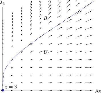
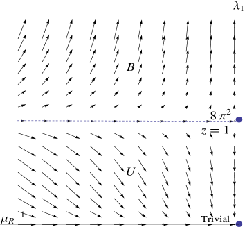
Figure 2: In the figure on the left are plotted RG flows in the $(\lambda_{3},\ \mu_{R})$ plane and in the one on the right are flows in the $(\lambda_{1},\ 1/\mu_{R})$ plane. $\mu_{R}$ increases from left to right in both figures. The chiral symmetry broken (unbroken) phase is indicated by the letter B (U). The dotted line is the critical curve on which $\phi_{0}$ vanishes.

In the broken phase, on the critical line $\phi_{R}=0$, the RG flow from UV ends on the Lorentz invariance violating fixed point in the IR. This can be seen directly from (39). Making the change of variables $k_{4}\rightarrow Ek_{4},\ k\rightarrow Ek/|g_{1}|$ in this equation, we get

$$\frac{1}{\lambda_{1}}=2\int\frac{[d^{4}k]_{1}}{(2\pi)^{4}}\ \frac{k_{4}^{2}+\tilde{l}_{R}^{2}(k)-\phi_{R}^{2}}{(k_{4}^{2}+\tilde{l}_{R}^{2}(k)+\phi_{R}^{2})^{2}}+\frac{|g_{1}|^{3}}{E^{2}}\xi,$$ (50)

where, as before, $\tilde{l}_{R}(k)=k(\epsilon k^{2}/\mu_{R}^{2}+1)$ and $\int[d^{4}k]_{1}\ \cdots=\int d^{4}k\ \theta(1-(k_{4}^{2}+\tilde{l}_{R}^{2}(k)))\ \cdots$. Now, in the broken phase, the gap equation implies $\xi=0$. So, for $\mu_{R}^{-1}=\phi_{R}=0$, the right-hand side of the above equation evaluates to $1/8\pi^{2}$. What happens for $\mu_{R}^{-1}=0$, but $\phi_{R}\neq 0$? In this case, for small values of $\phi_{R}$, the coupling increases as $\lambda_{1}\sim 8\pi^{2}/(1-\phi_{R}^{2}{\rm ln}\phi_{R}^{-2})$. So, these trajectories diverge to larger values of the coupling, doing so faster for larger values of $\phi_{R}$. Figure 2 confirms this for trajectories in the broken phase. Note that there is no fixed point for $\lambda_{1}\rightarrow\infty$ since the beta function of $\lambda_{1}^{-1}$ does not vanish at $\lambda_{1}^{-1}=0$.

In the unbroken phase, $|g_{1}|^{3}\xi$ is a non-zero constant, independent of the flow parameter $E$, while $E\rightarrow 0$ in the IR. Thus, in the unbroken phase the RG flow will terminate at $\lambda_{1}=0$ in the IR.

What does the theory look like at these two fixed points? Consider first the nontrivial fixed point at $\lambda_{1}=8\pi^{2}$. The fixed point action can be obtained from (44) by setting $\phi_{R}=0$ and taking the limit $\mu_{R}\rightarrow\infty$. For $\phi_{R}=0$, the fermions become massless. In the $\sigma$ kinetic terms, the coefficients $\bar{C}_{1,2}$ grow logarithmically in the limit $\mu_{R}\rightarrow\infty$, as shown in (67). The implication is that as we approach the fixed point $\lambda_{1}=8\pi^{2}$, the kinetic terms for $\sigma$ grow and eventually dominate the mass term. This can be seen more directly by the rescaling $\sigma\rightarrow\sigma/\sqrt{\bar{C}_{1}}$. In the limit $\mu_{R}\rightarrow\infty$, the mass term and the Yukawa interaction disappear, leaving behind a massless scalar decoupled from the fermions. So the theory at this fixed point has free massless fermions and a free massless scalar, the maximum attainable velocity of the latter being different from the former, unless $\bar{\mu}\gg 1$, in which case Lorentz invariance is restored near the fixed point.

Note that our analysis implies the existence of a fixed point in the usual relativistic NJL model as well. This can be established as follows. The RG equation for the 4-fermi coupling in the NJL model can be obtained by setting $\bar{\mu}\gg 1$ and $z=1$ in (42). Since $\mu_{R}\gg\bar{\mu}$, this also implies $\mu_{R}\gg 1$. For large $\mu_{R}$ and $z=1$, the equation for $\lambda_{1}=\lambda_{R}/|g_{1R}|^{3}$ is precisely (49). Moreover, from the low energy action (44), we see that in this parameter regime the Lorentz violating piece in the fermion kinetic term vanishes and the coefficients $\bar{C}_{1,2}$ work out to be those appropriate for a relativistic NJL model with a cut-off $\Lambda$, as we have argued below equation (67).

The other fixed point, that at $\lambda_{1}=0$, is described by just a free massless fermion. This is because near this fixed point the $\sigma$ mass goes to infinity as $\mu_{R}^{2}$ because of the manner in which $\lambda_{1}$ approaches the fixed point, which is described by equation (50). Therefore, this time the rescaling $\sigma\rightarrow\sigma/\sqrt{\bar{C}_{1}}$ leaves the mass term as dominant, with the mass going to infinity. Hence $\sigma$ decouples at the fixed point, leaving behind free massless relativistic fermions. This is the theory that one gets from the original four-fermi model at the trivial (Gaussian) fixed point.

5 Concluding remarks

In this paper we have analysed RG flows in a $z=3$ Lifshitz-like four fermi model, which is ultraviolet complete in $3+1$ dimensions. The model flows in the infrared to a theory in which Lorentz invariance is violated at ${\cal O}(1)$ level, which cannot be tuned away by adjusting a parameter. The origin of these violations can be traced to fermions with energies higher than the Lorentz violating energy scale, propagating in loops and contributing to the induced kinetic terms for the composite boson, in the chiral symmetry broken vacuum. However, if one works with a finite cut-off, which is taken to be much smaller than the Lorentz invariance violating scale, then the model flows in the infrared to an approximately Lorentz invariant theory even in the bosonic sector, which is similar to the low energy limit of the usual Nambu$-$Jona-Lasinio model in the broken phase. A physical way of interpreting the cut-off could be as supersymmetry breaking scale in a supersymmetric version of this model. In this case, the offending contributions of fermions in loops would be cancelled by their supersymmetric partners and the Lorentz violations would be controlled by the ratio of the Lorentz violating scale to the supersymmetry breaking scale, which can, in principle, be made small. Possible applications of the present model to the Higgs sector of the Standard Model would then put constraints on these two scales for consistency with data.

A remarkable feature of the general RG equations we have obtained, (32) and (36), is that they describe flow in two scaling parameters, namely $a$ and $b$. More generally, in a theory with anisotropy in $n$ different directions, the RG equations will describe flow in $n$ parameters. The parameters presumably get related near a fixed point, as in the present example in which we found that $a=b^{\frac{1}{z}}$ near the fixed point labeled by the exponent $z$. Away from the fixed points, however, a more general flow in multiple scaling parameters would seem to be more appropriate. It would be interesting to explore such more general flows.

6 Acknowledgements

We would like to thank Spenta Wadia for a collaboration at an early stage of this work and for numerous discussions. We would also like to thank Sumit Das, Alfred Shapere, Juan Maldacena, Shiraz Minwalla and Michael Peskin for discussions. G.M. would like to thank the organizers of the Benasque conference on Gravity (July 2009), the organizers of the QTS6 meeting in Lexington, the University of Kentucky, Lexington and the School of Natural Sciences, IAS, Princeton for hospitality during part of this project.

Appendix A Coefficients appearing in the vacuum solution

We give here the coefficients $I_{0},~{}I_{1},~{}I_{2}$ and $I_{3}$ that appeared in equation (20):

$$\kern-18.0ptI_{0}\equiv\int_{0}^{1}dk\frac{k^{4}}{1+g_{0}^{2}k^{6}}=\frac{1}{12g_{0}^{5/3}}\biggl{(}2\tan^{-1}{\frac{3g_{0}^{1/3}(1-g_{0}^{2/3})}{1+g_{0}^{4/3}-4g_{0}^{2/3}}}+\sqrt{3}\ln{\frac{1+g_{0}^{2/3}-\sqrt{3}g_{0}^{1/3}}{1+g_{0}^{2/3}+\sqrt{3}g_{0}^{1/3}}}\biggr{)},$$

$$\kern-18.0ptI_{1}\equiv\int_{0}^{1}dk\frac{k^{2}}{1+g_{0}^{2}k^{6}}=\frac{1}{3g_{0}}\tan^{-1}{g_{0}},$$

$$\kern-18.0ptI_{2}\equiv\int_{0}^{1}dk\frac{k^{8}}{(1+g_{0}^{2}k^{6})^{2}}=\frac{1}{6g_{0}^{3}}\left(\tan^{-1}{g_{0}}-\frac{g_{0}}{1+g_{0}^{2}}\right),$$

$$\kern-18.0ptI_{3}\equiv\int_{0}^{1}dk\frac{k^{8}}{(1+g_{0}^{2}k^{6})^{3}}=\frac{1}{24g_{0}^{3}}\left(\tan^{-1}{g_{0}}+\frac{g_{0}^{3}-g_{0}}{(1+g_{0}^{2})^{2}}\right).$$ (51)

Appendix B Evaluation of the low energy effective action

Here we give some details of the calculation that lead to the low energy action (29). Integrating out the high energy modes of the fermions gives the effective action

$$\Delta S=-i~{}{\rm Tr}~{}\ln(A+B)=-i~{}{\rm Tr}~{}\ln(A)-i~{}{\rm Tr}~{}\ln(1+A^{-1}B)$$ (52)

where $A(k,q)\equiv(2\pi)^{4}\left(\gamma^{0}k_{0}-\vec{\gamma}.\vec{l}(\vec{k})+\phi_{0}\right)\delta^{4}(k-q)$, $B(k,q)\equiv\frac{1}{\sqrt{N}}\sigma(k-q)$ and ’Tr’ stands for integration over high momenta (between the lower cut-off $E$ and upper cut-off $\Lambda$, as explained above equation (29)) and trace over all indices. $\Delta S$ can be expanded as

$$\Delta S=-i~{}{\rm Tr}~{}\ln(A)-i~{}{\rm Tr}(A^{-1}B)+\frac{i}{2}{\rm Tr}(A^{-1}B)^{2}+~{}\text{higher powers}$$ (53)

Each factor of B comes with a factor of $\frac{1}{\sqrt{N}}$ and hence the “higher powers” of $(A^{-1}B)$ are subleading in $1/N$. Thus, powers higher than quadratic in $\sigma(k)$ in the effective action (29) are subleading in $1/N$, which we omit. Now,

$${\rm Tr}~{}\ln(A)=iNV\int\frac{[d^{4}k]_{E\rightarrow\Lambda}}{(2\pi)^{4}}\quad{\rm tr}~{}\ln\left(\gamma^{0}k_{0}-\vec{\gamma}.\vec{l}(\vec{k})+\phi_{0}\right),$$ (54)

where ‘tr’ stands for trace over Dirac indices only. Also, ${\rm Tr}(A^{-1}B)$ is given by

$${\rm Tr}(A^{-1}B)=4i\phi_{0}\sqrt{N}\sigma(k=0)\int\frac{[d^{4}k]_{E\rightarrow\Lambda}}{(2\pi)^{4}}\ \frac{1}{k_{4}^{2}+l^{2}(k)+\phi_{0}^{2}},$$ (55)

where we have continued the momenta to the Euclidean signature. Thus, the coefficient $C_{3}$ appearing in (29) is given by

$$C_{3} \kern-18.0pt=\frac{1}{\lambda}-2\int\frac{[d^{4}k]_{E\rightarrow\Lambda}}{(2\pi)^{4}}\ \frac{1}{k_{4}^{2}+l^{2}(k)+\phi_{0}^{2}}.$$ (56)

Now,

$$\kern-18.0pt{\rm Tr}(A^{-1}B)^{2}=\int\frac{[d^{4}p]_{E}}{(2\pi)^{4}}|\sigma(p)|^{2}\int\frac{[d^{4}k]_{E\rightarrow\Lambda}}{(2\pi)^{4}}$$

$$\kern-18.0pt\times{\rm tr}~{}\frac{1}{\left\{\gamma^{0}k_{0}-\vec{\gamma}.\vec{l}(\vec{k})+\phi_{0}\right\}\left\{\gamma^{0}(k_{0}-p_{0})-\vec{\gamma}.\vec{l}(\vec{k}-\vec{p})+\phi_{0}\right\}}$$

Expanding to quadratic order in $p_{0},|\vec{p}|$ for small values, the above expression gives

$$\frac{i}{2}{\rm Tr}(A^{-1}B)^{2}= \kern-18.0pt\int\frac{[d^{4}p]_{E}}{(2\pi)^{4}}|\sigma(p)|^{2}\biggl{\{}C_{1}p_{0}^{2}-C_{2}p^{2}+2\int\frac{[d^{4}k]_{E\rightarrow\Lambda}}{(2\pi)^{4}}\ \frac{k_{4}^{2}+l^{2}(k)-\phi_{0}^{2}}{\left(k_{4}^{2}+l^{2}(k)+\phi_{0}^{2}\right)^{2}}\biggr{\}}$$

Thus, the action will be of the form given by equation (29) where $C_{0}$ is given by

$$C_{0}=\frac{1}{\lambda}-2\int\frac{[d^{4}k]_{E\rightarrow\Lambda}}{(2\pi)^{4}}\ \frac{k_{4}^{2}+l^{2}(k)-\phi_{0}^{2}}{\left(k_{4}^{2}+l^{2}(k)+\phi_{0}^{2}\right)^{2}}.$$ (57)

Moreover, the coefficients $C_{1,2}$ are given by

$$C_{1}(g_{0},g_{1};\Lambda,E,\phi_{0})=\int\frac{[d^{4}k]_{E\rightarrow\Lambda}}{(2\pi)^{4}}\biggl{\{}-2\Delta^{2}+4\left(l^{2}(k)+4\phi_{0}^{2}\right)\Delta^{3}$$

$$\hskip 199.16928pt-16\phi_{0}^{2}\left(l^{2}(k)+\phi_{0}^{2}\right)\Delta^{4}\biggr{\}},$$ (58)

$$C_{2}(g_{0},g_{1};\Lambda,E,\phi_{0})=\int\frac{[d^{4}k]_{E\rightarrow\Lambda}}{(2\pi)^{4}}\biggl{\{}A_{2}(k)\Delta^{2}-A_{3}(k)\Delta^{3}+A_{4}(k)\Delta^{4}\biggr{\}},$$

$$~{}~{}~{}~{}A_{2}(k)=2(g_{0}k^{2}+g_{1})(2g_{0}k^{2}+g_{1})+\frac{4}{3}g_{0}k^{2}(5g_{0}k^{2}+3g_{1}),$$

$$~{}~{}~{}~{}A_{3}(k)=\frac{4}{3}l^{2}(k)(3g_{0}k^{2}+g_{1})^{2}+4\phi_{0}^{2}(g_{0}k^{2}+g_{1})(3g_{0}k^{2}+g_{1})$$

$$~{}~{}~{}~{}\hskip 36.98866pt+\frac{8}{3}g_{0}\phi_{0}^{2}k^{2}(6g_{0}k^{2}+4g_{1}),$$

$$~{}~{}~{}~{}A_{4}(k)=\frac{16}{3}\phi_{0}^{2}l^{2}(k)(3g_{0}k^{2}+g_{1})^{2},$$ (59)

where $\Delta(k_{4},k)=1/(k_{4}^{2}+l^{2}(k)+\phi_{0}^{2})$.

For nonzero values of $g_{0}$ and $g_{1}$, one can express the dependence of $C_{1,2}$ on these parameters essentially only through one combination, the scale $\mu$ defined in (27). For example, one can scale out the dependence on $g_{1}$. This can be done by the change of the integration variable $k\rightarrow k/|g_{1}|$. We get

$$C_{1}(g_{0},g_{1};\Lambda,E,\phi_{0})=|g_{1}|^{-3}C_{1}(\epsilon\mu^{-2},1;\Lambda,E,\phi_{0})\equiv|g_{1}|^{-3}\bar{C}_{1},$$

$$C_{2}(g_{0},g_{1};\Lambda,E,\phi_{0})=|g_{1}|^{-1}C_{2}(\epsilon\mu^{-2},1;\Lambda,E,\phi_{0})\equiv|g_{1}|^{-1}\bar{C}_{2}.$$ (60)

where $\epsilon=\pm 1$ is the relative sign of $g_{0}$ and $g_{1}$. In terms of the dimensionless renormalized parameters defined in (31) and (35), it is easy to show that

$$\bar{C}_{1,2}=C_{1,2}(\epsilon\mu_{R}^{-2},1;\mu_{R}/\bar{\mu},1,\phi_{R})=C_{1,2}(\epsilon,1;1/\bar{\mu},1/\mu_{R},\bar{\phi}/\bar{\mu}),$$ (61)

where $\bar{\phi}=\phi_{0}/\Lambda$ and $\bar{\mu}=\mu/\Lambda$ are the values of the respective running couplings, $\phi_{R},\ \mu_{R}$, at the UV cut-off. The form in the second equality will be useful later when we discuss the $E\rightarrow 0$ limit of these coefficients. Now, from the first equality of (61) and (60), we get

$$\bar{C}_{1}=|g_{1R}|^{3}C_{1}(g_{0R},g_{1R};\mu_{R}/\bar{\mu},1,\phi_{R})\equiv|g_{1R}|^{3}C_{1R},$$

$$\bar{C}_{2}=|g_{1R}|C_{2}(g_{0R},g_{1R};\mu_{R}/\bar{\mu},1,\phi_{R})\equiv|g_{1R}|C_{2R}.$$ (62)

Similarly, scaling out the dependence on $g_{0}$, we get

$$C_{1}(g_{0},g_{1};\Lambda,E,\phi_{0})=|g_{0}|^{-1}C_{1}(\epsilon,\mu^{\frac{2}{3}};\Lambda,E,\phi_{0}),$$

$$C_{2}(g_{0},g_{1};\Lambda,E,\phi_{0})=|g_{0}|^{-1/3}C_{2}(\epsilon,\mu^{\frac{2}{3}};\Lambda,E,\phi_{0}).$$ (63)

Moreover, one can easily show that in terms of the renormalized parameters,

$$C_{1}(\epsilon,\mu^{\frac{2}{3}};\Lambda,E,\phi_{0})=E^{-2}C_{1}(\epsilon,\mu_{R}^{\frac{2}{3}};\mu_{R}/\bar{\mu},1,\phi_{R})\equiv C_{1}^{\prime}/E^{2},$$

$$C_{2}(\epsilon,\mu^{\frac{2}{3}};\Lambda,E,\phi_{0})=E^{-2/3}C_{2}(\epsilon,\mu_{R}^{\frac{2}{3}};\mu_{R}/\bar{\mu},1,\phi_{R})\equiv C_{2}^{\prime}/E^{2/3}$$ (64)

Then, from (62)-(64), one gets

$$C_{1}^{\prime}=\bar{C}_{1}/\mu_{R}^{2},\qquad C_{2}^{\prime}=\bar{C}_{2}/\mu_{R}^{\frac{2}{3}}.$$ (65)

It is easy to see that $C_{1,2}^{\prime}$ are finite for $\mu_{R}=0$. It follows that the quantities on right-hand side of equations in (65) have a finite limit as $\mu_{R}\rightarrow 0$.

Appendix C Limiting behaviour of $\bar{C}_{1,2}$

Here we will discuss the limiting behaviour of the coefficients $\bar{C}_{1,2R}$, given by (58), (59) and (61), for large values of $\mu_{R}$, which is the IR regime of small $E$. We first note that for any positive real number $\eta$ satisfying $\bar{\mu}^{-1}>\eta^{-1}>\mu_{R}^{-1}$, we have $(\int[d^{4}k]_{\mu_{R}^{-1}\rightarrow\bar{\mu}^{-1}}\ \cdots)=(\int[d^{4}k]_{\eta^{-1}\rightarrow\bar{\mu}^{-1}}\ \cdots)-(\int[d^{4}k]_{\mu_{R}^{-1}\rightarrow\eta^{-1}}\ \cdots)$. It follows from this identity and the second equality of (61) that

$$\bar{C}_{1,2}=C_{1,2}(\epsilon,1;1/\bar{\mu},1/\eta,\bar{\phi}/\bar{\mu})+C_{1,2}(\epsilon,1;1/\eta,1/\mu_{R},\bar{\phi}/\bar{\mu})$$ (66)

We are interested in the limit of large $\mu_{R}$ for $\bar{\phi}=0$. The $\mu_{R}$ dependence of $\bar{C}_{1,2}$ comes only from the second term above. In the limit $1\gg\eta^{-1}>\mu_{R}^{-1}$, the calculation of this term greatly simplifies since the “higher derivative” terms can be neglected. That is, in this regime of parameter values, $k\ll 1$ throughout the integration range, so we may neglect $k^{2}$ compared to $1$. Then, from (58) and (59), we find that the leading contribution goes as

$$\bar{C}_{1,2}\approx C_{1,2}(\epsilon,1;1/\bar{\mu},1/\eta,0)+\frac{1}{8\pi^{2}}{\rm ln}\left(\frac{\mu_{R}}{\eta}\right).$$ (67)

We see that $\bar{C}_{1,2}$ grow logarithmically with $\mu_{R}$. If $\bar{\mu}\gg 1$, then we may choose $\eta=\bar{\mu}$. In this case, $\bar{C}_{1}\approx\bar{C}_{2}\approx\frac{1}{8\pi^{2}}{\rm ln}\left(\mu_{R}/\bar{\mu}\right)$. These are just the values for these coefficients in the relativistic NJL case. However, in general, $\bar{C}_{1}$ is quite different from $\bar{C}_{2}$ and both are quite different from the corresponding quantities in the relativistic NJL case. Therefore, in general the $\sigma$ kinetic terms do not have Lorentz symmetry, as discussed in section 3 below equation (30).

References

- [1] R. M. Hornreich, M. Luban and S. Shtrikman, “Critical Behavior at the Onset of -Space Instability on the Line,” Phys. Rev. Lett. 35, 1678 (1975).
- [2] R. Sachdev, “Quantum Phase Transitions,” Cambridge University Press (1999).
- [3] E. Ardonne, P. Fendley and E. Fradkin, “Topological order and conformal quantum critical points,” Annals Phys. 310, 493 (2004) [arXiv:cond-mat/0311466].
- [4] S. Papanikolaou, E. Luijten, Eduardo Fradkin, “Quantum criticality, lines of fixed points, and phase separation in doped two-dimensional quantum dimer models,” Phys. Rev. B 76, 134514 (2007) [arXiv:cond-mat/0607316]
- [5] Luiz C. de Albuquerque, Marcelo M. Leite, “Uniaxial Lifshitz Point at ,” [arXiv:cond-mat/0006462].
- [6] D. T. Son, “Quantum critical point in graphene approached in the limit of infinitely strong Coulomb interaction,” Phys.Rev. B75 (2007) 235423 [arXiv:cond-mat/0701501].
- [7] D. T. Son, “Toward an AdS/cold atoms correspondence: a geometric realization of the Schroedinger symmetry,” Phys. Rev. D 78, 046003 (2008) [arXiv:0804.3972 [hep-th].
- [8] K. Balasubramanian and J. McGreevy, “Gravity duals for non-relativistic CFTs,” Phys. Rev. Lett. 101, 061601 (2008) [arXiv:0804.4053 [hep-th].
- [9] S. Kachru, X. Liu and M. Mulligan, “Gravity Duals of Lifshitz-like Fixed Points,” Phys. Rev. D 78, 106005 (2008) [arXiv:0808.1725 [hep-th].
- [10] M. Taylor, “Non-relativistic holography,” arXiv:0812.0530 [hep-th].
- [11] T. Azeyanagi, W. Li and T. Takayanagi, “On String Theory Duals of Lifshitz-like Fixed Points,” arXiv:0905.0688 [hep-th].
- [12] W. Li, T. Nishiyoka and T. Takayanagi, “Some No-go Theorems for String Duals of Non-relativistic Lifshitz-like Theories,” IPMU09-0090, KUNS-2224 [arXiv:0908.0363].
- [13] E. J. Brynjolfsson, U. H. Danielsson, L. Thorlacius and T. Zingg, “Holographic Superconductors with Lifshitz Scaling,” arXiv:0908.2611 [hep-th].
- [14] K. Balasubramanian and J. McGreevy, “An analytic Lifshitz black hole,” arXiv:0909.0263 [hep-th].
- [15] S. A. Hartnoll, “Lectures on holographic methods for condensed matter physics,” Class. Quant. Grav. 26, 224002 (2009) [arXiv:0903.3246 [hep-th]].
- [16] P. Horava, “Quantum Criticality and Yang-Mills Gauge Theory,” arXiv:0811.2217 [hep-th].
- [17] M. Visser, “Lorentz symmetry breaking as a quantum field theory regulator,” Phys. Rev. D 80, 025011 (2009) [arXiv:0902.0590 [hep-th]].
- [18] B. Chen and Q. G. Huang, “Field Theory at a Lifshitz Point,” arXiv:0904.4565 [hep-th].
- [19] A. Dhar, G. Mandal and S. Wadia “Asymptotically free four-fermi theory in 4 dimensions at the z=3 Lifshitz-like fixed point,” Phys. Rev. D 80, 105018 (2009) [arXiv:0905.2928 [hep-th]]
- [20] S. R. Das and G. Murthy, “ Models at a Lifshitz Point,” Phys. Rev. D 80, 065006 (2009) [arXiv:0906.3261 [hep-th]].
- [21] Roberto Iengo, Jorge G. Russo, Marco Serone, “Renormalization group in Lifshitz-type theories,” arXiv:0906.3477.
- [22] D. Orlando and S. Reffert, “On the Perturbative Expansion around a Lifshitz Point,” arXiv:0908.4429 [hep-th].
- [23] S. R. Das and G. Murthy, “Compact Electrodynamics in 2+1 dimensions: Confinement with gapless modes,” arXiv:0909.3064 [hep-th].
- [24] J. Alexandre, K. Farakos, P. Pasipoularides and A. Tsapalis, “Dynamical generation of Lorentz symmetry for a Lifshitz-type Yukawa model,” arXiv:0909.3719 [hep-th].
- [25] W. Chao, “The Hierarchy Problem and Lifshitz Type Quantum Field Theory,” arXiv:0911.4709 [hep-th].
- [26] P. Horava, “Quantum Gravity at a Lifshitz Point,” Phys. Rev. D 79, 084008 (2009) [arXiv:0901.3775 [hep-th]].
- [27] C. Charmousis, G. Niz, A. Padilla and P. M. Saffin, “Strong coupling in Horava gravity,” JHEP 0908 (2009) 070 [arXiv:0905.2579 [hep-th]].
- [28] M. Li and Y. Pang, “A Trouble with Horava-Lifshitz Gravity,” arXiv:0905.2751 [hep-th].
- [29] D. Blas, O. Pujolas and S. Sibiryakov, “On the Extra Mode and Inconsistency of Horava Gravity,” JHEP 0910 (2009) 029 [arXiv:0906.3046 [hep-th]].
- [30] C. Bogdanos and E. N. Saridakis, “Perturbative instabilities in Horava gravity,” arXiv:0907.1636 [hep-th].
- [31] D. Blas, O. Pujolas and S. Sibiryakov, “A healthy extension of Horava gravity,” arXiv:0909.3525 [hep-th].
- [32] K. Koyama and F. Arroja, “Pathological behaviour of the scalar graviton in Horava-Lifshitz gravity,” arXiv:0910.1998 [hep-th].
- [33] A. Papazoglou and T. P. Sotiriou, “Strong coupling in extended Horava-Lifshitz gravity,” arXiv:0911.1299 [hep-th].
- [34] D. Anselmi, “Weighted power counting, neutrino masses and Lorentz violating extensions of the Standard Model,” Phys.Rev.D79:025017,2009 and arXiv:0808.3475 [hep-ph].
- [35] D. Anselmi, “Standard Model Without Elementary Scalars And High Energy Lorentz Violation,” arXiv:0904.1849 [hep-ph].
- [36] Y. Kawamura, “Misleading Coupling Unification and Lifshitz Type Gauge Theory,” arXiv:0906.3773.
- [37] Kunio Kaneta, Yoshiharu Kawamura, “Fermion Mass Hierarchy in Lifshitz Type Gauge Theory,” arXiv:0909.2920.
- [38] Y. Nambu and G. Jona-Lasinio, “Dynamical model of elementary particles based on an analogy with superconductivity. I,” Phys. Rev. 122, 345 (1961).
- [39] S. Liberati and L. Maccione, “Lorentz Violation: Motivation and new constraints,” arXiv:0906.0681 [astro-ph.HE].
- [40] J. Bolmont, R. Buhler, A. Jacholkowska and S. J. Wagner [the H.E.S.S. Collaboration], “Search for Lorentz Invariance Violation effects with PKS 2155-304 flaring period in 2006 by H.E.S.S,” arXiv:0904.3184 [gr-qc].
- [41] L. Gonzalez-Mestres, “AUGER-HiRes results and models of Lorentz symmetry violation,” Nucl. Phys. Proc. Suppl. 190, 191 (2009) [arXiv:0902.0994 [astro-ph.HE]].
- [42] S. T. Scully and F. W. Stecker, “Lorentz Invariance Violation and the Observed Spectrum of Ultrahigh Energy Cosmic Rays,” Astropart. Phys. 31, 220 (2009) [arXiv:0811.2230 [astro-ph]].
- [43] G. Altarelli, “Particle Physics at the LHC Start,” arXiv:0902.2797 [hep-ph].