A polarizable interatomic force field for TiO₂ parameterized using density functional theory

Abstract

We report a classical interatomic force field for TiO₂, which has been parameterized using density functional theory forces, energies, and stresses in the rutile crystal structure. The reliability of this new classical potential is tested by evaluating the structural properties, equation of state, phonon properties, thermal expansion, and some thermodynamic quantities such as entropy, free energy, and specific heat under constant volume. The good agreement of our results with ab initio calculations and with experimental data, indicates that our force-field describes the atomic interactions of TiO₂ in the rutile structure very well. The force field can also describe the structures of the brookite and anatase crystals with good accuracy.

I Introduction

Recently, a bipolar switching phenomenon in TiO₂ has been observed jeong1 ; jeong2 ; shima and much work has been done to design superior TiO₂-based resistive random access memory (RRAM) devices. This, together with many other important applications of TiO₂, such as white pigment for paints, sunscreen, high-efficiency solar cells regan , and photosplitting of water to hydrogen khan ; du , has been stimulating a great deal of research interest in atomistic simulations of TiO₂. Accurate atomistic simulations would provide detailed information at the atomic level that might answer some important open questions, such as the mechanism of bipolar switching.

Force fields are the key to accurate atomistic simulations. In the last twenty years, many force fields have been built for TiO₂ matsui ; swamy ; ogata ; collins ; hallil ; kerisit ; thomas ; tetot . Among these, the partial-charge rigid-ion model of Matsui and Akaogi (MA model) matsui , and the variable-charge Morse stretch (MS-Q) interatomic potential of Swamyswamy , have been the most successful and popular. Both the MA and MS-Q models can describe a series of crystal structures quite well. A common feature of these force fields is that they were adapted to reproduce experimental bulk properties, such as lattice constants, cohesive energies, bulk moduli and elastic constants. An alternative parameterization method consists of fitting force fields to forces, energy differences, and stresses extracted from ab initio calculations ercolessi ; ts ; ts-mgo ; brommer . To our knowledge, no such ab initio force field for TiO₂ yet exists.

Having a potential that can accurately model the vibrational properties of TiO₂ as well as its structures is very important as they determine its finite-temperature macroscopic properties. The phonon dispersion curves and density of states for rutile TiO₂ have been measured by the coherent inelastic scattering of thermal neutrons along principal symmetry directions of the Brillouin zone traylor . The $\Gamma$-point phonons have been measured by Raman porto and infrared spitzer spectroscopy. In addition to these experimental determinations, phonon frequencies have been calculated ab initiomontanari ; lee ; sikora . However, little attention has been paid to the determination of phonon properties from a force field for TiO₂, even though it is a very demanding test of a force field’s accuracy. As has been demonstrated for MgOts-mgo ; aguado , ab initio-based classical force fields have the potential to give a very good description of phonon properties. TiO₂ has several competing lattice structures and is a more complex oxide than MgO. It is rather interesting, therefore, to see how well such a force field can predict its vibrational properties.

In this work, we present a polarizable classical interatomic force field for TiO₂, parameterized from ab initio calculations. We test its accuracy by comparing its predictions of structural properties, equations of state, phonon frequencies, and the temperature dependences of lattice parameters, entropy, free energy, and specific heat under constant volume in the rutile phase with experimental data and with ab initio calculations. We also calculate the structures and relative energies of the brookite and anatase phases to get an indication of the force field’s transferability.

II Force field

The potential energy function $U=U^{\textrm{sr}}+U^{\textrm{es}}$ that we use to describe interactions between ions consists of a pairwise term $U^{\textrm{sr}}$ describing short-range non-electrostatic interactions and an electrostatic term $U^{\textrm{es}}$ describing dipole induction and the electrostatic interactions of the charges and induced dipole moments of the ions.

For the short-range interaction energy we use the pairwise Morse-stretch form

$$U^{\textrm{sr}} = \sum_{i>j}D_{ij}\big{[}e^{\gamma_{ij}[1-(r_{ij}/r_{ij}^{0})]}-2e^{(\gamma_{ij}/2)[1-(r_{ij}/r_{ij}^{0})]}\big{]}$$ (1)

where $r_{ij}=|{\bf r}_{i}-{\bf r}_{j}|$ is the distance between nearby ions $i$ and $j$ and $D_{ij}$, $\gamma_{ij}$, and $r_{ij}^{0}$ are parameters that are specific to the pair of species of ions $i$ and $j$. This potential is truncated at a radius of $18.0$ a.u.

The total electrostatic contribution to the energy of the system includes charge-charge, charge-dipole, and dipole-dipole interaction terms:

$$U^{\textrm{es}} = \frac{1}{4\pi\epsilon_{0}}\sum_{i>j}\bigg{[}\frac{q_{i}q_{j}}{r_{ij}}+\sum_{\gamma}\nabla_{\gamma}\bigg{(}\frac{1}{r_{ij}}\bigg{)}\big{(}p_{i}^{\gamma}q_{j}-q_{i}p_{j}^{\gamma}\big{)}$$ (2)

$$- \sum_{\gamma,\beta}\nabla_{\beta}\nabla_{\gamma}\bigg{(}\frac{1}{r_{ij}}\bigg{)}p_{i}^{\gamma}p_{j}^{\beta}\bigg{]}+\sum_{i,\gamma}\frac{(p_{i}^{\gamma})^{2}}{2\alpha_{i}}$$

where $q_{i}$ is the charge of ion $i$, $p_{i}^{\gamma}$ is the $\gamma^{\textrm{th}}$ cartesian component of the dipole moment of ion $i$, $\alpha_{i}$ is its polarisability, and $\nabla_{\gamma}=\partial/\partial r^{\gamma}_{ij}$. The final term on the right hand side of this equation is a sum of the self energies of the ions. The self energy of an ion is the internal energy cost of inducing a dipole on it.

There are two mechanisms for the induction of ionic dipole moments. The first is via the short-range repulsive forces between ions which can distort an ion’s electron cloud thereby giving it a dipole moment. The second is the induction of a dipole moment on an ion by the electric field arising from the charges and the dipole moments of all other ions.

To model the induction by short-range repulsive forces we follow the approach of Madden et al.wilson-madden1 ; rowley . In their approach, the contribution of the short-range forces to dipole moments is given by

$${\bf p_{i}^{\text{sr}}}=\alpha_{i}\sum_{j\neq i}\frac{q_{j}{\bf r}_{ij}}{r_{ij}^{3}}f_{ij}(r_{ij})$$ (3)

where

$$f_{ij}(r_{ij})=c_{ij}\sum_{k=0}^{4}\frac{(b_{ij}r_{ij})^{k}}{k!}e^{-b_{ij}r_{ij}}$$ (4)

and $b_{ij}$ and $c_{ij}$ are model parameters.

The electrostatically-induced dipole moments are more difficult to calculate because they are all interdependent due to their contributions to, and dependences on, the electric field. At every time step we find the dipole moments of the ions by iterating to self-consistency the equation

$${\bf p}_{i}^{m}=\alpha_{i}{\bf E}({\bf r}_{i};\{{\bf p}_{j}^{m-1}\}_{j\neq i};\{{\bf r}_{j}\}_{j\neq i})+{\bf p}_{i}^{\text{sr}}$$ (5)

where ${\bf p}_{i}^{m}$ is the dipole moment on ion $i$ at iteration $m$ of the self-consistent cycle; ${\bf E}({\bf r}_{i})$ is the electric field at position ${\bf r}_{i}$.

We use Ewald summation to calculate electrostatic energies, forces, stresses, and electric fields.

Our model depends on a set of parameters $\{\eta_{n}\}$ comprising the Morse-Stretch parameters $D$, $\gamma$, and $r^{0}$, the parameters $b$ and $c$ of the short-range dipole model, and the charges $q_{\textrm{\tiny Ti}},q_{\textrm{\tiny O}}$ and polarisabilities $\alpha_{\textrm{\tiny Ti}},\alpha_{\textrm{\tiny O}}$ of the ions. In section III we describe how these parameters are determined.

III Potential parameterization

III.1 Ab initio molecular dynamics

Total energies, stresses, and forces are computed from ab initio simulations based on density functional theory (DFT). Ab initio molecular dynamics (MD) simulations employing the projector augmented wave method (PAW) were performed in the NVT ensemble under periodic boundary conditions using the VASP simulation package vasp1 ; vasp2 ; vasp3 . Only the Ti (3d,4s) and O (2s,2p) electron states were treated as valence states, however, tests in which the Ti (3s, 3p) semicore states were included yielded similar results for the energy differences between crystalline phases and the phonon frequencies of rutile TiO₂. The local-density approximation (LDA) to the exchange-correlation energy was used. The velocity Verlet algorithm verlet with a time step of $1$ fs was adopted to solve the equations of motion, and temperature was controlled using a Nose-Hoover thermostatnose . We used a $2\times 2\times 3$ supercell that contained $72$ atoms and only the $\Gamma$-point was used to sample the Brillouin zone. A kinetic energy cutoff of $180$ eV was used in the plane-wave expansion of the wave functions during the MD simulations. The goal of these ab initio MD simulations was simply to produce some reasonable atomic configurations to serve as representative snapshots at finite temperature. These configurations were then used to perform higher-precision DFT calculations of forces, stresses, and energies for use in the force-field parameterization.

III.2 Fitting procedure for the potential

We fit our potential to DFT calculations in the rutile crystal structure, however, to broaden the range of different environments for the ions, two temperatures are considered in the potential fitting: 300K and 1000K. Furthermore, at each temperature, configurations at more than one volume were chosen. For 300K eight configurations were used. Six of these configurations are taken from an ab initio MD simulation at the zero temperature equilibrium volume. The other two were obtained from simulations in which the volume was expanded by 3%. At 1000K, we used 3 sets of data in total, each containing four configurations. These three sets are obtained from MD simulations at the zero-temperature equilibrium volume, and at volumes expanded by 3% and by 9%. To minimize correlations between configurations, successive snapshots were separated from one another by 2 ps of ab initio MD. For each snapshot, we used VASP to calculate the forces, energies and stresses. To obtain these quantities with high precision, the Brillouin zone was sampled using a $2\times 2\times 2$ Monkhorst-Pack $k-$point mesh and, to converge the forces and the stress tensors properly, a very high wavefunction cutoff energy of $1500$ eV was used.

The potential parameters were obtained by minimizing the cost function

$$\Gamma(\{\eta_{n}\})=w_{f}\Delta F+w_{s}\Delta S+w_{e}\Delta E$$ (6)

with respect to the parameters $\{\eta_{n}\}$ where

$$\Delta F = \frac{\sqrt{\sum_{k=1}^{N_{c}}\sum_{I=1}^{N}\sum_{\alpha}|F_{cl,I}^{\alpha}(\{\eta_{n}\})-F_{ai,I}^{\alpha}|^{2}}}{\sqrt{\sum_{k=1}^{n_{c}}\sum_{I=1}^{N}\sum_{\alpha}(F_{ai,I}^{\alpha})^{2}}}$$ (7)

$$\Delta S = \frac{\sqrt{\sum_{k=1}^{N_{c}}\sum_{\alpha,\beta}|S_{cl}^{\alpha\beta}(\{\eta_{n}\})-S_{ai}^{\alpha\beta}|^{2}}}{3B\sqrt{n_{c}}}$$ (8)

$$\Delta E = \frac{\sqrt{\sum_{k,l}^{N_{c}}((U_{k}^{cl}-U_{l}^{cl})-(U_{k}^{ai}-U_{l}^{ai}))^{2}}}{\sqrt{\sum_{k,l}^{n_{c}}(U_{k}^{ai}-U_{l}^{ai})^{2}}}$$ (9)

$F_{cl,i}^{\alpha}$ is the $\alpha$-component of the force on ion $i$ calculated with the classical potential; $F_{ai,i}^{\alpha}$ is the $\alpha$-component of the force on ion $i$ calculated ab initio; $S_{cl}^{\alpha\beta}$ is the stress tensor component calculated with the classical potential; $S_{ai}^{\alpha\beta}$ is the stress tensor component calculated ab initio; $N_{c}$ denotes the number of snapshot configurations used in the fit; $B$ is the bulk modulus; $U_{cl}^{k}$ is the potential energy of configuration $k$ for the classical potential, and $U_{ai}^{k}$ is its energy calculated ab initio. $w_{f}$, $w_{s}$, and $w_{e}$ are weights that quantify the relative importances to the fitting cost function of forces, stresses, and energies, respectively. In this work, $w_{f}=1.0$, $w_{s}=0.5$, and $w_{e}=0.01$. These numbers are somewhat arbitrary as long as the energy differences are given a relatively small weight because we only have one energy per configuration. We tried different weights and found no significant difference in the final values of $\Delta F$, $\Delta S$, and $\Delta E$. Minimization of $\Gamma(\{\eta_{n}\})$ is performed by a combination of simulated annealing simann and Powell minimizationnumrec . The former is used to provide an initial parameter set which brings the cost function to a basin in the surface defined by $\Gamma(\{\eta_{n}\})$ in $\eta-$space. Minimization is then completed using Powell’s method.

We assume that DFT provides accurate atomic forces and energies. Therefore if, at the global minimum of $\Gamma$ in $\eta-$space, $\Delta F$ remains large it means that the potential model does not contain the ingredients necessary to fit the DFT potential energy surface closely. The model is unphysical or incomplete and the resulting force-field is unlikely to produce results that are in good agreement with experiment. Agreement with experiment can still be found by fitting to experimental data, but when agreement is not attributable to accurate interatomic forces, it is difficult to place confidence in the force-field for calculations that can not be directly checked by comparison with experiment. However, when reliable experimental data is available, simulations are of limited value anyway. For this reason we deem it important for a force-field to be able to fit DFT forces closely and the closeness of the fit achieved in the parameterisation is itself a test of the quality of the potential.

IV Results

Following the fitting procedure described in the previous section, we obtained the force-field parameters for rutile TiO₂, as listed in table 1. In this fitting, $\Delta F=0.202$, $\Delta S=0.009$, and $\Delta E=0.046$. Put another way, the root-mean-squared error in the forces is $20.2\%$ of the root-mean-squared force.

As a comparison we have checked how close the MA model’s forces are to the ab initio ones. We find that the root-mean-squared difference between the MA forces and the DFT forces is $\sim 88\%$ of the root-mean-squared DFT forces ($\Delta F\approx 0.88$, $\Delta S\approx 0.02$, $\Delta E\approx 0.63$). The MA model uses the pairwise Born-Mayer potential form and by minimising $\Gamma$ with respect to the parameters of the Born-Mayer potential we have been able to achieve a best fit of $\Delta F\approx 0.48$, $\Delta S\approx 0.01$, $\Delta E\approx 0.10$. However, this resulted in a disimprovement in the description of the three crystal structures with respect to the MA potential. As one might expect, and as was found previously for silicats , when the fit to ab initio calculations is poor, the ability of a potential to reproduce experimental results does not correlate with the quality of the fit. Our tests strongly suggest that the Born-Mayer form provides a poor microscopic description of atomic forces in TiO₂.

IV.1 Crystal structures

In order to check the reliability and transferability of the new force field, we computed the structural properties of three different crystalline polymorphs of TiO₂, namely the rutile, anatase, and brookite structures. Structural optimizations for these three crystals were performed via the steepest-descent method at zero pressure. The resulting lattice parameters are presented in Table 2 and compared to the ab initio data calculated with the VASP package and to experimental dataabrahams ; burdett ; meagher , both at room temperature and (for rutile and anatase) at $15$ K. Both ab initio calculations and the new force field reproduce experimental data quite well and the accuracy of the force field is comparable to that of DFT. We stress that the force field in this work is only fit to ab initio data from calculations in the rutile crystal structure. Therefore, its ability to reproduce the structures of anatase and brookite is an indication that it may be reasonably transferable between different structures. However, apart from the handful of structural and energetic properties presented in this paper, we have not tested the force field in these phases.

Parameters	O-O	Ti-O	Ti-Ti
$D$	$1.5865\times 10^{-3}$	$1.7668\times 10^{-3}$	$5.0276\times 10^{-3}$
$\gamma$	9.6370	12.2332	5.9069
$r^{0}$	6.5150	4.7678	8.1380
$b$	1.5368	4.8187	1.8246
$c$	2.9216	-122.1489	-0.7918
$\alpha$	2.9314		10.2739
$q$	-1.1045		2.209

Table 1: The fitted interatomic force-field parameters (in atomic units).

	a (Å)			b (Å)			c (Å)
	Exp.	DFT-LDA	POT	Exp.	DFT-LDA	POT	Exp.	DFT-LDA	POT
Rutile
$\sim$ 0 K	4.587burdett	4.571	4.494				2.959burdett	2.925	3.015
$\sim$ 300 K	4.593burdett		4.504				2.954burdett		3.023
Anatase
$\sim$ 0 K	3.782burdett	3.821	3.790				9.512burdett	9.694	9.292
$\sim$ 300 K	3.785burdett						9.502burdett
Brookite
$\sim$ 0 K		9.1197	9.095		5.415	5.399		5.103	5.131
$\sim$ 300 K	9.174meagher			5.449meagher			5.138meagher

Table 2: Lattice parameters for three optimised structures of TiO₂, together with experimental data and results from ab initio calculations. DFT-LDA represents ab initio calculations with the VASP package within the local density approximation, and POT the new force field, obtained by fitting to ab initio data in the rutile structure. Data at two temperatures are presented, where available: at close to 0 K (15 K in the experiment of Ref. burdett, , 0 K for simulation) and at room temperature.

	V0/TiO2 (Å3)		B0 (GPa)			B${}^{*}_{0}$
	DFT-LDA	POT	Exp.	DFT-LDA	POT	DFT-LDA	POT
Rutile	30.62	30.46	211$\pm$ 7ming	252	241	5.37	5.07
			230$\pm$ 20gerward
Anatase	33.58	33.37	178swamy	188	171	1.75	2.34
Brookite	31.55	31.50	no data	230	196	3.87	3.14

Table 3: Birch-Murnaghan EOS parameters for different structures of TiO₂, together with the experimental data available. Experimental data refers to room temperature, while theoretical values are obtained at $0$ K.

	Experiment	DFT-LDA	DFT-GGA	POT	MA
E${}_{\text{anatase}}$-E${}_{\text{rutile}}$	35.0mitsuhashi , 53.8navrotsky	-12.0	-81.2	425.9	301.6
E${}_{\text{brookite}}$-E${}_{\text{rutile}}$	7.7mitsuhashi	-17.5	-39.9	212.6	179.3

Table 4: Energy differences in meV/TiO₂ between the anatase and brookite crystal structures and the rutile crystal structure. The experiments of reference navrotsky, and the calculations with the MA modelmatsui were performed at room temperature, while the more recent experiments of reference mitsuhashi, were performed at $971$ K. The experiments measured enthalpies of transformation whereas all the DFT and force-field calculations that we report are energy differences at $0$ K.

IV.2 Equations of state

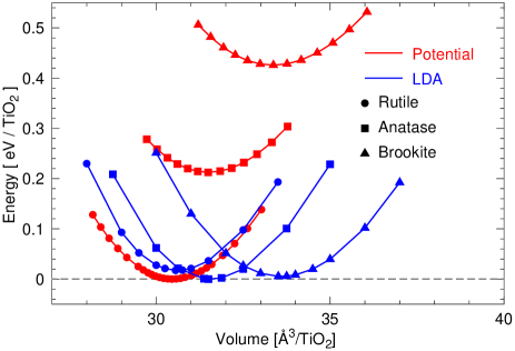
Figure 1: Volume dependence of the energy of TiO₂ in the rutile, brookite, and anatase crystal structures for our potential (red lines) and from LDA ab initio calculations. Energies are expressed relative to the equilibrium energy of the most stable phase.

The energy as a function of volume for all three phases has been calculated with our potential and the results are illustrated in Fig. 1. Structural relaxations were performed at each volume. The results in red are from the new force field, while those in blue are from our density functional theory calculations within the local density approximation (DFT-LDA). In each case, we set the energy of the most stable phase in equilibrium to zero. We can see that the DFT-LDA calculations and the new force field give similar equilibrium volumes for the three crystals (Table 3). However, it is clear from Fig. 1 and Table 4, that the energy sequences obtained from DFT-LDA calculations and the new force field are different and, furthermore, that the the magnitudes of the energy differences between the three structures differ substantially between DFT-LDA and our force field. In DFT-LDA calculations, the energy differences between the three structures are small, and $E_{\text{brookite}}<E_{\text{anatase}}<E_{\text{rutile}}$. However, for the new potential, the rutile structure is the ground state, and $E_{\text{rutile}}<E_{\text{brookite}}<E_{\text{anatase}}$. While this energy ordering is consistent with the experimental results mitsuhashi ; navrotsky the magnitudes of the energy differences are at least an order of magnitude too large. The DFT-LDA estimates of the magnitudes of the energy differences, both here and in previous worklabat , are in much better agreement with experiment, despite the fact that they predict the wrong sequence of structures. We have also calculated the equilibrium energy differences within a generalized gradient approximation (GGA)pbe to the exchange-correlation energy. The GGA differences in energy between anatase and rutile and between brookite and rutile are also presented in Table 4. The magnitudes of these energy differences are larger than those of LDA, but still a factor of $\sim 5$ smaller than we find with our force field. We are unaware of compelling reasons why LDA should outperform GGA for TiO₂. Therefore, it seems reasonable to consider differences between LDA and GGA as lower bounds on the error bars associated with our approximation to the exchange-correlation energy. The free-energy differences calculated with the MA model at room temperature are similar in magnitude (but slightly smaller) to the $0$ K energy differences calculated with our force field and the MA model’s energy ordering of the three crystal structures is also consistent with experiment. Although our force field produces energy differences that are much too large, it is at least gratifying that the crystal structures have the correct energy sequence.

The relationship between energy and volume can be described by the Birch-Murnaghan equation of statebirch

$$E(V)-E_{0} = \frac{9V_{0}B_{0}}{16}\Bigg{\{}\Bigg{[}\bigg{(}\frac{V_{0}}{V}\bigg{)}^{\frac{2}{3}}-1\Bigg{]}^{3}B_{0}^{*}$$ (10)

$$+ \Bigg{[}\bigg{(}\frac{V_{0}}{V}\bigg{)}^{\frac{2}{3}}-1\Bigg{]}^{2}\Bigg{[}6-4\bigg{(}\frac{V_{0}}{V}\bigg{)}^{\frac{2}{3}}\Bigg{]}\Bigg{\}}$$

where $V$ is the volume, $V_{0}$ the equilibrium volume, $E_{0}$ the equilibrium energy, $B_{0}$ the bulk modulus, and $B_{0}^{*}$ the pressure derivative of the bulk modulus. The parameters for the equation of state are listed in Table 3, together with experimental data ming ; gerward ; swamy . The results from the ab initio calculations, the new classical potential, and the experimental data are all in good agreement, however, it is important to note that the simulation results refer to zero temperature while the experiments were performed at room temperature.

IV.3 Vibrational properties of rutile

To have a further test of the new force field, the phonons of rutile TiO₂ are calculated with the small displacement method implemented by Togo’s FROPHO package togo . Figure 2(a) compares phonons calculated with our classical potential (black dots) with those calculated from DFT-LDA (green triangles) and, for some branches and symmetry directions, with inelastic neutron data at room temperature taken from reference traylor, . Figure 2(b) shows the same ab initio and experimental data, but the black dots are now from calculations using the MA modelmatsui . We include in both these plots only those frequencies calculated for phonons whose wavelengths are commensurate with our simulation cells, i.e., no interpolation has been performed to infer frequencies at different wavevectors. Simulations with the classical potentials were performed with three different simulation supercells whose sizes, in multiples of the primitive $6$-atom unit cell, were $14\times 14\times 14$ ($16464$ atoms), $12\times 12\times 12$ ($10368$ atoms), and $10\times 10\times 10$ ($6000$ atoms). Our DFT calculations were performed in a $4\times 4\times 4$ ($384$ atoms) supercell.

In our calculations we have corrected longitudinal optical frequencies in the long wavelength limit (i.e. ${\bf k}\rightarrow 0$) to account for the effects of the long-range electric fields that these modes induce born-huang ; togo .

The first thing to note from Figures 2(a) and 2(b) is that both classical potentials struggle to reproduce the dispersion of the acoustic modes close to the zone boundaries. This can be seen most clearly along the $\Gamma\rightarrow A$ and $\Gamma\rightarrow Z$ symmetry directions. However, what is also clear is that our force field greatly improves on the MA model in this respect. For the high-frequency modes, between $\sim 15$ THz and $\sim 25$ THz, our model is in very good agreement with experiment and with DFT. The MA model’s description of the phonon spectrum at these frequencies is very poor by comparison. Overall, it is clear that our potential provides a description of the phonon spectrum that is much better than that provided by the MA model. It is also clear, however, that there is room for improvement, presumably by improving the functional form of the potential.

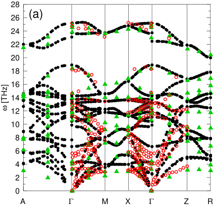
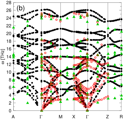
Figure 2: Phonon dispersion curves of TiO₂ in the rutile crystal structure from different methods. (a)Results from our new force field (black dots) compared to experimenttraylor (red circles) and ab initio (DFT-LDA) calculations (green triangles). (b)Results from the MA force field (black dots) compared to experimenttraylor (red circles) and ab initio (DFT-LDA) calculations (green triangles).

IV.4 “Electronic” properties

To correct the LO frequencies at the $\Gamma$-point, it has been necessary to calculate the high-frequency dielectric tensor ${\bf\varepsilon}_{\infty}$, which is diagonal, and the Born effective charge tensor ${\bf Z}^{*}$. We have calculated ${\bf\varepsilon}_{\infty}$ and ${\bf Z}^{*}$ directly by calculating the polarization responses to small electric fieldsliang and to small displacements of the atoms, respectively. In the rutile crystal structure we find the components of ${\bf\varepsilon}_{\infty}$ perpendicular and parallel to the c-axis to be $\varepsilon_{\perp}=2.58$ and $\varepsilon_{\parallel}=2.75$, respectively, which is in poor agreement with those calculated ab initiorignanese ($\varepsilon_{\perp}=7.49$, $\varepsilon_{\parallel}=8.57$). The Born effective charge tensor of rutile has only three independent non-zero components for each atom. We calculate them to be $Z^{*}_{xx}(\text{Ti})=Z^{*}_{yy}(\text{Ti})=3.428$, $Z^{*}_{xy}(\text{Ti})=Z^{*}_{yx}(\text{Ti})=0.422$, $Z^{*}_{zz}(\text{Ti})=3.789$ and $Z^{*}_{xx}(\text{O})=Z^{*}_{yy}(\text{O})=-1.714$, $Z^{*}_{xy}(\text{O})=Z^{*}_{yx}(\text{O})=-1.044$, $Z^{*}_{zz}(\text{O})=-1.895$. Again, this is in poor agreement with the ab initio resultsrignanese which are $Z^{*}_{xx}(\text{Ti})=Z^{*}_{yy}(\text{Ti})=6.36$, $Z^{*}_{xy}(\text{Ti})=Z^{*}_{yx}(\text{Ti})=1.00$, $Z^{*}_{zz}(\text{Ti})=7.52$ and $Z^{*}_{xx}(\text{O})=Z^{*}_{yy}(\text{O})=-3.18$, $Z^{*}_{xy}(\text{O})=Z^{*}_{yx}(\text{O})=-1.81$, $Z^{*}_{zz}(\text{O})=-3.76$. Our potential is not intended to give a good description of the electronic properties of the system, so this disagreement is no cause for concern. We intend, instead, an accurate representation of the interatomic forces. Both $Z^{*}$ and $\varepsilon_{\infty}$ are derivatives of the polarization field, and are therefore only meaningful on length scales that are large compared to the primitive unit cell of the crystal. At large distances, forces between atoms (labeled ‘1’ and ‘2’) are proportional to $Z^{*}_{1}Z^{*}_{2}/\varepsilon_{\infty}$, and so this is the relevant quantity if one is interested assessing the quality of these response functions’ contributions to interatomic forces. Therefore, we look at the components of the screened effective charge tensor $Z^{*}_{\alpha\beta}/\sqrt{\varepsilon_{\gamma\delta}}$. The symmetry of the crystal is such that, for each atomic species, there are only three non-unique non-zero components of the screened effective charge tensor: $Z^{*}_{xx}/\sqrt{\varepsilon_{\perp}}=Z^{*}_{yy}/\sqrt{\varepsilon_{\perp}}$, $Z^{*}_{xy}/\sqrt{\varepsilon_{\perp}}=Z^{*}_{yx}/\sqrt{\varepsilon_{\perp}}$, and $Z^{*}_{zz}/\sqrt{\varepsilon_{\parallel}}$.

	DFT		POT
	Ti	O	Ti	O
$Z^{*}_{xx}/\sqrt{\varepsilon_{\perp}}=Z^{*}_{yy}/\sqrt{\varepsilon_{\perp}}$	2.32	-1.16	2.13	-1.07
$Z^{*}_{xy}/\sqrt{\varepsilon_{\perp}}=Z^{*}_{yx}/\sqrt{\varepsilon_{\perp}}$	0.37	-0.66	0.26	-0.65
$Z^{*}_{zz}/\sqrt{\varepsilon_{\parallel}}$	2.57	-1.28	2.28	-1.14

Table 5: Components of the screened effective charge tensor calculated with density functional theory (DFT) and with our new potential (POT)

We have calculated these quantities, which determine long-range forces, with our force field and, in Table 5, we compare our results to those obtained from DFT. The agreement between our potential and DFT is good, therefore our potential should describe long-range forces reasonably well.

The best-fit ionic polarisabilities ( $\alpha_{\text{O}}=2.9$ a.u., $\alpha_{\text{Ti}}=10.3$ a.u.) (Table 1) provided by our parameterization process are unusual and worthy of comment. The polarisability of the oxygen ion is much lower than has been found by force fitting for other oxides such as MgOts-mgo and SiO₂ts , or from electronic structure simulationsaguado . Typically, $\alpha_{\text{O}}$ is between $5$ and $15$ a.u.. However, most surprising is the large polarizability of the Ti ions. One would expect a small polarizability for a cation, particularly one with such a high positive charge.

By making atoms polarisable, we include the response of electrons in a phenomenological way. However, we only include one response mechanism. Others, such as higher-order polarisabilities and charge-transfer between ions, are certain to exist to some degree. Furthermore, we are using a fully-ionic model while covalent effects might be important. It seems likely that including one or more of these effects would allow our parameterizer to achieve a closer fit to the ab initio forces. We speculate that the strange polarisabilities are an effort by our parameterization program to compensate for those other electronic effects which are not present in the mathematical form of the potential. It is remarkable, and further evidence of the power of the force-fitting approach, that the parameteriser succeeds in finding values for the charges and polarisabilities of the atoms that perform so well.

IV.5 Thermal expansion

Figure 3 compares the dependence of the lattice parameters of the rutile structure on temperature with experimentkrishna ; meagher . Once again, the agreement is very good, indicating that the anharmonicity of the potential energy surface is well reproduced by our force field. The results reported in figure 3 were from long ($>100$ ps) MD simulations of a $6\times 6\times 8$ supercell, which contains $1728$ atoms. A time step of $0.723$ fs was used and temperature was controlled with a Nose-Hoover thermostatnose . While atoms moved according to Newton’s equations (using a Verlet algorithm), steepest descent was performed on the cell degrees of freedom. We verified that this approach gave almost identical results to performing Parrinello-Rahman constant pressure simulationspr and taking averages over the trajectory of the lattice constants. However, the latter simulations are more time consuming and more difficult to control. We caution that our simulations treat the ions purely classically and that quantum effects would flatten out these curves at low temperatures.

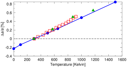
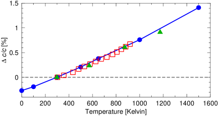
Figure 3: Temperature dependence of the lengths of the rutile lattice vectors, expressed as percentage differences with respect to their room temperature values, i.e. $\Delta a(T)=a(T)-a(300\text{ K})$. Boxes and filled triangles refer to the experimental data of Refs. krishna, and meagher, , respectively. Blue dots are the results of MD simulations with our new force field.

IV.6 Thermodynamic properties

Thermodynamic properties of rutile TiO₂, such as free energy, entropy, and phonon specific heat under constant volume were evaluated in the quasi-harmonic approximation from the phonons using the FROPHO package togo and the results are given in Figure 4. We compare the results from DFT calculations of the phonons and calculations of the phonons with our force field. In both cases, phonons were calculated in $4\times 4\times 4$ supercell. As illustrated in Figure 4(a), the temperature dependence of the free energy calculated from the new force field is almost the same as that from our ab initio calculation. An enlargement of the free energy curve is also superimposed in Figure 4(a) in order to see the difference between these two results more clearly. The entropy of rutile TiO₂ is given in Figure 4(b). Again, the new force field reproduces the ab initio calculation extremely well.

Figure 4(c) shows that the specific heat under constant volume ($C_{v}$) from the new classical force field is also in excellent agreement with our ab initio calculations. Within the Debye model debye , $C_{v}(T)$ can be expressed as

$$C_{v}=9Nk_{B}\bigg{(}\frac{T}{T_{D}}\bigg{)}^{3}\int_{0}^{T_{D}/T}\frac{x^{4}e^{x}}{(e^{x}-1)^{2}}dx$$ (11)

where $N$ is the number of atoms per cell (6 for rutile TiO₂), $k_{B}$ is the Boltzmann constant, and $T_{D}$ is the Debye temperature. Using this expression, the specific heat at $T_{D}$ can be computed as

$$C_{v}(T=T_{D})=9Nk_{B}\int_{0}^{1}\frac{x^{4}e^{x}}{(e^{x}-1)^{2}}dx=17.1312k_{B}$$ (12)

By comparing this value with our calculation, we can obtain the Debye temperature $T_{D}$. We find that our ab initio calculations predict $T_{D}=781.6$ K while our new force field predicts $T_{D}=786.1$ K. These values are very close to the experimental Debye temperature of $778.3$ K porto .

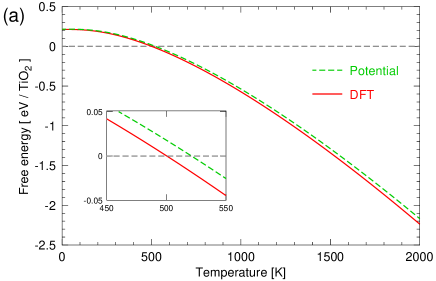
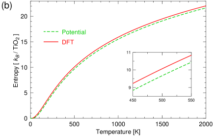
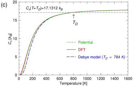
Figure 4: Thermodynamic properties of rutile TiO₂ derived from phonon properties: (a) free energy $F$; (b) entropy $S$; (c) specific heat $C_{v}$ under constant volume

V Conclusions

A new classical force field for TiO₂ has been proposed that has been parameterized using forces, stresses, and energies extracted from ab initio molecular dynamics simulations. The potential can not only predict the structural properties of TiO₂ in three crystal structures, namely, rutile, brookite, and anatase, but also gives the right ground state and the correct energy sequence of these three structures and predicts their bulk moduli with an accuracy comparable to DFT. While the force field has been constructed with rutile in mind, and fit to ab initio data of the rutile structure, it seems likely to be reasonably transferable to different structures. However, the most obvious deficiency of the force-field is that it overestimates energy differences between these polymorphs. This, and the unphysical polarisabilities of the ions, suggest that our functional form may lack ingredients necessary to describe some electronic effects that can play important roles in the energetics of TiO₂. Quadrupole polarisation of ions and dynamical charge transfer between ions are two effects that may have an important role to play.

Concerning the vibrational properties, the new potential can reproduce most features of ab initio and experimental results, and is a substantial improvement over the widely-used MA model for TiO₂. Furthermore, the potential provides an excellent description of the temperature dependence of the rutile lattice constants. The good description of vibrational properties from the proposed force field is further confirmed by thermodynamic quantities calculated from the phonon properties. The calculated free energy, entropy, specific heat under constant volume, and Debye temperature via the new classical force field are in excellent agreement with those from ab initio calculations.

Overall, our results indicate that the force field presented provides a very accurate description of atomic interactions in rutile TiO₂. The force field can be applied with some confidence to studies of bulk properties of titania. While further testing is necessary, we can also hope that it provides an improved description of surface properties. If this is the case, it can be used to study, not only surfaces, but also nanocrystals and nanowires, all of which have huge technological importance for their catalytic and optical properties.

We stress that no experimental data, other than the rutile crystal symmetry, has been used to parameterize this potential, therefore, we can be confident that its predictive capability is based on a robust description of the ions’ potential-energy surface.

VI Acknowledgments

X. J. H. acknowledges useful discussions with H. Schober. P.T. acknowledges useful discussions with M. W. Finnis and N. M. Harrison. L.B. acknowledges support from the EU within the Marie Curie Actions for Human Resources and Mobility. P.T. acknowledges support from the European Commission within the Marie Curie Support for Training and Development of Researchers Programme under Contract No. MIRG-CT-2007-208858.

References

- (1) D. S. Jeong, H. Schroeder, and R. Waser, Phys. Rev. B 79, 195317 (2009).
- (2) D. S. Jeong, H. Schroeder, and R. Waser, Electrochem. Solid-State Lett. 10, G51 (2007).
- (3) H. Shima, N. Zhong, and H. Akinaga, Appl. Phys. Lett. 94, 082905 (2009).
- (4) B. O’Regan and M. Grätzel, Nature 353, 737 (1991).
- (5) S. U. M. Khan, M. Al-Shahry, W. B. Ingler Jr., Science 297, 2243 (2002).
- (6) Y. Du, N. A. Deskins, Z. Zhang, Z. Dohnalek, M. Dupuis, and I. Lyubinetsky, Phys. Rev. Lett. 102, 096102 (2009).
- (7) M. Matsui, and M. Akaogi, Mol. Simu. 6, 239 (1991).
- (8) V. Swamy, J. D. Gale, and L. S. Dubrovinsky, J. Phys. Chem. Solids 62, 887 (2001).
- (9) S. Ogata, H. lyetomi, K. Tsuruta, F. Shimojo, R. K. Kalia, A. Nakano, and P. Vashishta, J. Appl. Phys. 86, 3036 (1999).
- (10) D. R. Collins, W. Smith, Council for the Central Laboratory of the Research Councils Tech. Rep. DL-TR-96-001, 1996.
- (11) A. Hallil, R. Tétot, F. Berthier, I. Braems, and J. Creuze, Phys. Rev. B 73, 165406 (2006).
- (12) S. Kerisit, N. A. Deskins, K. M. Rosso, and M. Dupuis, J. Phys. Chem. C 112, 7678 (2008).
- (13) B. S. Thomas, N. A. Marks, and B. D. Begg, Phys. Rev. B 69, 144122 (2004).
- (14) R. Tétot, A. Hallil, J. Creuze, and I. Braems, Europhys. Lett. 83 40001, (2008).
- (15) F. Ercolessi and J. B. Adams, Europhys. Lett. 26, 583 (1994).
- (16) P. Tangney and S. Scandolo, J. Chem. Phys. 117, 8898 (2002).
- (17) P. Tangney and S. Scandolo, J. Chem. Phys. 119, 9673 (2003).
- (18) P. Brommer and F. Gähler, Modelling Simul. Mater. Sci. Eng. 15, 295 (2007).
- (19) J. G. Traylor, H. G. Smith, R. M. Nicklow, and M. K. Wilkinson, Phys. Rev. B 3, 3457 (1971).
- (20) S. P. S. Porto, P. A. Fleury, T. C. Damen, Phys. Rev. 154, 522 (1962).
- (21) W. G. Spitzer, R. C. Miller, D. A. Kleinman, and L. E. Howarth, Phys. Rev. 126, 1710 (1962).
- (22) B. Montanari and N. M. Harrison, Chem. Phys. Lett. 364, 528 (2002).
- (23) C. Lee, P. Ghosez, and X. Gonze, Phys. Rev. B 50, 13379 (1994).
- (24) R. Sikora, J. Phys. Chem. Sol. 66, 1069 (2005).
- (25) A. Aguado and P. A. Madden, Phys. Rev. B 70, 245103 (2004).
- (26) M. Wilson and P. A. Madden, J. Phys: Cond. Matt. 5, 2687 (1993).
- (27) A. J. Rowley, P. Jemmer, M. Wilson, and P. A. Madden, J. Chem. Phys. 108, 10209 (1998).
- (28) G. Kresse and J. Hafner, Phys. Rev. B 47, 558 (1993).
- (29) G. Kresse and J. Furthmüller, Phys. Rev. B 54, 11169 (1996).
- (30) G. Kresse and D. Joubert, Phys. Rev. B 59, 1758 (1999).
- (31) L. Verlet, Phys. Rev. 159, 98 (1967); Phys. Rev. 165, 201 (1967).
- (32) S. Nosé, J. Chem. Phys. 81, 511 (1984); S. Nose, Mol. Phys. 52, 255 (1984); W. G. Hoover, Phys. Rev. A 31, 1695 (1985).
- (33) S. Kirkpatrick, C. D. Gelatt, and M. P. Vecchi, Science 220, 671 (1983).
- (34) W. H. Press, W. T. Vetterling, B. P. Flannery, and S. A. Teukolsky, Numerical Recipes in Fortran 77 and Fortran 90: The Art of Scientific and Parallel Computing, 2nd ed. (Cambridge University Press, Cambridge, 1996).
- (35) S. C. Abrahams, J. L.Bernstein, J. Chem. Phys. 55, 3206 (1971)
- (36) J. K. Burdett, T. Hughbanks, G. J. Miller, J. W. Richardson, and J. V. Smith, J. Am. Chem. Soc. 109, 3639 (1987).
- (37) E. P. Meagher and G. A. Lager, Canad. Mineral. 17, 77 (1979).
- (38) T. Mitsuhashi and O. J. Kleppa, J. Amer. Ceram. Soc. 62, 356 (1979).
- (39) A. Navrotsky and O. J. Kleppa, J. Amer. Ceram. Soc. 50, 626 (1967); A. Navrotsky, J. C. Jamieson, and O. J. Kleppa, Science 158 388 (1967).
- (40) F. Labat, P. Baranek, C. Domain, C. Minot, and C. Adamo, J. Chem. Phys. 126, 154703 (2007).
- (41) J. P. Perdew, K. Burke, and M. Ernzerhof, Phys. Rev. Lett. 77, 3865 (1996).
- (42) F. Birch, Phys. Rev. 71, 809 (1947).
- (43) L. Ming and M. H. Manghnani, J. Geophys. Res. 84, 4777 (1979).
- (44) L. Gerward and J. S. Olsen, J. Appl. Crystallogr. 30, 259 (1997).
- (45) A. Togo, FROPHO: Phonon analyser for periodic boundary condition materials; A. Togo, F. Oba, and I. Tanaka, Phys. Rev. B 78, 134106 (2008).
- (46) M. Born and K. Huang, Dynamical Theory of Crystal Lattices, Oxford Univ. Press, 1954.
- (47) P. Debye, Ann. Phys. 39, 789 (1912).
- (48) K. V. Krishna Rao, S. V. Nagender Naidu, and L. Iyengar, J. Amer. Cer. Soc. 53, 124 (1970).
- (49) Y. Liang, C. R. Miranda, and S. Scandolo, J. Chem. Phys. 125, 194524 (2006).
- (50) G.-M. Rignanese, X. Rocquefelte, X. Gonze, and A. Pasquarello, Int. J. Quant. Chem. 101, 793 (2005).
- (51) M. Parrinello and A. Rahman, Phys. Rev. Lett. 45, 1196 (1980).