Series Parallel Linkages

Abstract.

We study spaces of realisations of linkages (weighted graphs) whose underlying graph is a series parallel graph. In particular, we describe an algorithm for determining whether or not such spaces are connected.

1. Introduction

Let $G$ be a graph with vertex set $V$ and edge set $E$. Let $l:E\rightarrow\mathbb{R}^{\geq 0}$ (where $\mathbb{R}^{\geq 0}$ denotes the nonnegative real numbers). We will call $l$ a length function. We will call such a pair, $(G,l)$, a linkage. Note that this is not standard terminology. However, it seems appropriate in the given context to formalise the intuition that a weighted graph is the mathematical model for a mechanical linkage consisting of hinges and bars that are constrained to move in a plane (we ignore the issue of self intersections).

Given such a linkage $L=(G,l)$ we define the space of planar configurations of $L$ as follows:

$$C(L)=C(G,l):=\{p:V\rightarrow\mathbb{R}^{2}:|p(u)-p(v)|=l(\{u,v\})\forall\{u,v\}\in E\}$$

where $|p(u)-p(v)|$ denotes the standard Euclidean distance between $p(u)$ and $p(v)$. By definition, $C(L)$ is a subset of $\mathbb{R}^{2|V|}$ and thus inherits a natural metric space structure. Observe that there is a canonical action of the group of orientation preserving isometries of the plane on $C(L)$. We define the the moduli space of the linkage, denoted by $M(L)$ or $M(G,l)$, to be the orbit space of this action. It is easy to see that if $G$ is connected then $M(L)$ is a compact real algebraic variety. In general, it is difficult to decide whether or not $M(L)$ is even nonempty. An element of $M(L)$ is called a realisation of the linkage $L$.

The problem of finding a realisation of $L$ is known as the molecule problem - see [MR1358807]. In the case where $M(L)$ is nonempty, it is difficult to say much about the topology of this space without imposing some restrictions on the structure of the underlying graph $G$. The case where $G$ is a polygonal graph (i.e. connected with every vertex of degree two) is quite well understood and much is known about the topology of $M(L)$ in this case. For example, we have the following (see Theorem 1.6 of [MR2076003], for example).

Theorem 1.

If $G$ is a polygonal graph, then $M(L)$ is nonempty if and only if the longest edge has length at most half the total length of all the edges. Moreover $M(L)$ is connected if and only if the sum of the lengths of the second and third longest edges is at most half of the total length of all the edges.

Indeed, much more detailed information about the topology of $M(L)$ is available when $G$ is polygonal. The homotopical and homological properties of these spaces are well understood - see [MR1133898], [MR1614965] or [MR2076003], for example. For an overview of some of the theory of polygonal linkages, we refer the reader to [MR2455573].

Our purpose in this paper is to study $M(L)$ where $G$ is a series parallel graph (see below for definitions). We will show that it is possible to easily determine, for a given series parallel graph $G$ and weight function $l$, whether or not $M(L)$ is nonempty and, in the case when it is nonempty, whether or not it is connected. The problem of deciding whether the space is connected or not is connected with the motion planning problem in robotics. The motion planning problem is concerned with the existence of a path betweeb two configurations of a robot. If we think of our linkages as a model for mechanical linkages, then the motion planning problem for this particular type of “robot” is equivalent to finding a continuous path in $M(L)$ with specified endpoints.

We will show that for the class of series parallel graphs these problems can be answered by considering a finite system of linear inequalities in the edge lengths. In contrast, we note that even for the complete graph on four edges, the smallest 2-connected graph which is not series parallel, it is necessary to solve a polynomial equation of total degree 6 (quartic in each variable) in the edge lengths to determine whether or not a realisation exists.

Throughout this paper we adopt the convention that $L=(G,l)$ and that $L_{i}=(G_{i},l_{i})$.

2. Series Parallel Graphs

In this section, we review the basic constructions and facts concerning the class of series parallel graphs. First, we fix some conventions regarding some standard graph theory. A graph is a pair $(V,E)$ where $E$ is a multiset of unordered pairs of distinct elements of $V$. Thus, in particular multiple edges with the same endpoints are allowed. However loops are not allowed. A path graph is a graph isomorphic to a graph with vertex set $\{1,\dots,n\}$ and edge set $\{\{i,i+1\}:i=1,\dots,n-1\}$. A path linkage is a linkage $(P,l)$ where $P$ is a path graph. A polygonal graph is a graph isomorphic to a graph with vertex set $\{1,\dots,n\}$ and edge set $\{\{i,i+1\}:i=1,\dots,n-1\}\cup\{\{n,1\}\}$. A polygonal linkage is a linkage $(G,l)$ where $G$ is a polygonal graph.

A two terminal graph (TTG) is an ordered triple $(G,s,t)$ where $s$ and $t$ are distinct vertices of $G$ called the source and the sink, respectively. Collectively $s$ and $t$ are called the terminal vertices of the TTG. Given TTGs $(G_{1},s_{1},t_{1})$ and $(G_{2},s_{2},t_{2})$ we can define the series composition $(G_{1},s_{1},t_{1})\circ(G_{2},s_{2},t_{2})$ to be the TTG

$$(G_{1}\cup_{t_{2}\sim s_{1}}G_{2},s_{2},t_{1})$$

where $G_{1}\cup_{t_{2}\sim s_{1}}G_{2}$ denotes the graph obtained by identifying the vertices $t_{2}$ and $s_{1}$. Also we define the parallel composition $(G_{1},s_{1},t_{1})\|(G_{2},s_{2},t_{2})$ to be the TTG

$$(G_{1}\cup_{s_{1}\sim s_{2},t_{1}\sim t_{2}}G_{2},s_{1},t_{1}).$$

See Figure 1 for an illustration of these constructions. Observe that the operation of parallel composition is a commutative associative operation on the class of TTGs. Thus, in particular, given TTGs $(G_{i},s_{i},t_{i})$ for $i=1,\dots,n$ we can unambiguously refer to the parallel composition

$$(G_{1},s_{1},t_{1})\|\dots\|(G_{n},s_{n},t_{n}).$$

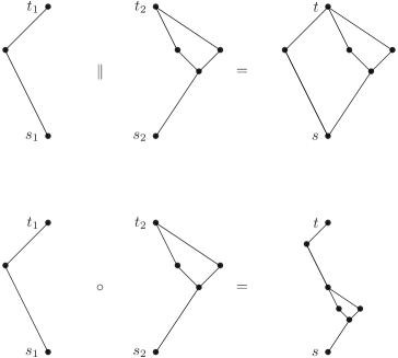
Figure 1. Parallel and series composition of two terminal graphs.

Let $K_{2}$ denote the complete graph with vertex set $\{s,t\}$. We define the class of two terminal series parallel graphs (TTSPGs) to be the smallest class of TTGs that contains $(K_{2},s,t)$ and that is closed under the operations of series and parallel composition. A series parallel graph is a graph $G$ such that $(G,s,t)$ is a TTSPG for some choice of vertices $s$ and $t$. Thus, for example, path graphs are series parallel. Also polygonal graphs are series parallel, since a polygon is the parallel composition of two paths. A series parallel linkage is a linkage $(G,l)$ such that $G$ is a series parallel graph. We note that the operations of parallel composition and series composition extend in an obvious way to linkages - so it makes sense to refer to the parallel composition $(L_{1},s_{1},t_{1})\|(L_{2},s_{2},t_{2})$ or the series composition $(L_{1},s_{1},t_{1})\circ(L_{2},s_{2},t_{2})$, where $L_{1}$ and $L_{2}$ are linkages rather than graphs.

Observe that for a given series parallel graph, there may be many possible choices of terminal vertices. However, the choice is not completely arbitrary - some pairs of vertices cannot be the terminal vertices of a given series parallel graph. For example, the existence of a subgraph of $G$ homeomorphic to

implies that $(G,u,v)$ is not a TTSPG. There are other possible obstructions. For a more detailed discussion of the possible choices of terminal vertices, see [MR1161075].

The following lemma will prove useful for our analysis of the connectedness of the moduli space of a series parallel linkage. Recall that a graph $G$ is 2-connected if the complement of any vertex is connected. Observe that a series parallel graph is 2-connected if and only if it cannot be expressed as a series composition of proper subgraphs.

Lemma 2.

Let $G$ be a 2-connected series parallel graph. There are vertices $s$ and $t$ in $G$ such that $(G,s,t)$ is a TTSPG and such that

$$(G,s,t)=(P_{1},s,t)\|(P_{2},s,t)\|(H,s,t),$$

where $P_{1}$ and $P_{2}$ are paths joining $s$ and $t$ and $H$ is a (possibly empty) subgraph of $G$ such that $(H,s,t)$ is a TTSPG.

Proof.

Let $P$ be a subgraph of $G$ such that $P$ is a path and such that every interior vertex of $P$ has degree 2 in $G$ (i.e. no other edges of $G$ are incident to the interior of $P$). Let $s$ and $t$ be the endpoints of $P$. By an easy modification of the proof of Lemma 9 in [MR1161075], we see that $(G,s,t)$ is a TTSPG (note that the hypothesis of 2-connectedness is necessary at this point) and thus $(G,s,t)=(P,s,t)\|(K,s,t)$. Here $K$ is the subgraph of $G$ spanned by all the edges that are not in $P$. Now it also easy to show (for example, by induction on the number of edges) that in any series parallel graph that is not itself a path graph, it is possible to find two distinct path subgraphs $P_{1}$ and $P_{2}$ with common endpoints and such that no other edges of $G$ are incident with any of the internal vertices of $P_{1}$ and $P_{2}$. Applying our previous observation to $P_{1}$ and $P_{2}$ completes the proof of the lemma. ∎

Series parallel graphs are a well studied class of graphs (see [MR849395] and [MR0175809] for example). Of particular interest to us is the following result of Belk and Connelly (see [MR2295049]). We say that a graph is $d$-realisable (where $d$ is a positive integer) if given any positive integer $n$ and any function $f:V\rightarrow\mathbb{R}^{n}$, there exists a function $g:V\rightarrow\mathbb{R}^{d}$ such that $|g(u)-g(v)|=|f(u)-f(v)|$ for all edges $\{u,v\}\in E$. Intuitively, this means that any embedding of $G$ into some (possibly high dimensional) Euclidean space can be squashed into $\mathbb{R}^{d}$ so that the edge lengths are preserved.

Theorem 3.

(Belk, Connelly) A graph is 2-realisable if and only if it is a series parallel graph.

Of course, knowing that a given graph $G$ is 2-realisable does not tell us whether or not $(G,l)$ is realisable for a particular length function $l$, nor does it tell us anything about the topology of $M(G,l)$. However Theorem 3 does suggest that the class of series parallel graphs is an interesting class for which to study the space $M(G,l)$.

3. realisability

Now suppose that $(G,s,t)$ is a TTSPG graph and that $l$ is a length function on $G$. Let $L$ be the linkage $(G,l)$. Let

$$[L,s,t]=\{|p(s)-p(t)|:p\in M(L)\}.$$

Here we are abusing notation somewhat by writing $p$ for an element of $M(P)$, but also using $p$ to denote a particular representative in $C(P)$ of the orbit under the action of orientation preserving isometries of $\mathbb{R}^{2}$. However, this clearly does not cause any problems with this definition as the quantity $|p(s)-p(t)|$ is preserved by this action. We will consistently abuse notation in this way throughout the remainder of the paper. In other words $[L,s,t]$ is the set of all possible values of the distance between $p(s)$ and $p(t)$ as $p$ varies over all realisations in $M(L)$. In the case where $L$ is a path linkage, there is only one possible choice for the set of terminal vertices, so we will write $[L]$ for $[L,s,t]$ in this case.

Note, that $[L,s,t]$ could be empty. Indeed, the linkage is realisable (i.e. $M(L)$ is nonempty) if and only if $[L,s,t]$ is nonempty.

We will show that it is possible to easily compute $[L,s,t]$ for a given TTSPG. Observe that in general it is difficult to compute the set of possible distances between a pair of points as we vary over all realisations of a (possibly non series parallel) graph. However for the special situation that we consider, it is possible.

Lemma 4.

Let $L_{1}=(G_{1},l_{1})$ and let $L_{2}=(G_{2},l_{2})$ and let $(G,s,t)=(G_{1},s_{1},t_{1})\|(G_{2},s_{2},t_{2})$. Then

$$[L,s,t]=[L_{1},s_{1},t_{1}]\cap[L_{2},s_{2},t_{2}].$$

In particular, $L$ is realisable if and only if $[L_{1},s_{1},t_{1}]\cap[L_{2},s_{2},t_{2}]$ is nonempty.

Proof.

If $x\in[L,s,t]$ then there is some $p\in M(L)$ such that $|p(s)-p(t)|=x$. For $i=1,2$, let $p_{i}=p|_{G_{i}}$. Now $x=|p_{i}(s)-p_{i}(t)|$, so $x\in[L_{i},s,t]$. This shows that $[L,s,t]\subseteq[L_{1},s,t]\cap[L_{2},s,t]$. For the other inclusion, suppose that $x\in[L_{1},s,t]\cap[L_{2},s,t]$. So, for $i=1,2$, there are realisations $p_{i}$ of $L_{i}$ such that $|p_{i}(s)-p_{i}(t|=x$. Clearly, $p_{1}$ and $p_{2}$ together induce a realisation $p$ of $L$ such that $|p(s)-p(t)|$. ∎

For series compositions, we make the following definition.

Definition 5.

Given intervals $[a,b]$ and $[c,d]$ with $0\leq a\leq b$ and $0\leq c\leq d$, define the composition $[a,b]\circ[c,d]$ to be the interval

$$[\max\{0,c-b,a-d\},b+d]$$

If we write $\phi$ to denote the empty interval, then we define $[a,b]\circ\phi:=\phi$.

Observe, for example, that $[a,b]\circ[c,d]=[0,b+d]$ if and only if $[a,b]\cap[c,d]$ is nonempty.

Lemma 6.

Let $L_{1}=(G_{1},l_{1})$ and $L_{2}=(G_{2},l_{2})$ be linkages such that $[L_{1},s_{1},t_{1}]$ and $[L_{2},s_{2},t_{2}]$ are both closed intervals. Let $(G,s_{2},t_{1})=(G_{1},s_{1},t_{1})\circ(G_{2},s_{2},t_{2})$. Then

$$[L,s_{2},t_{1}]=[L_{1},s_{1},t_{1}]\circ[L_{2},s_{2},t_{2}]$$

Proof.

This follows immediately from the observation that $x\in[L,s_{2},t_{1}]$ if and only if there is $y\in[L_{1},s_{1},t_{1}]$ and $z\in[L_{2},s_{2},t_{2}]$ such that $x$, $y$ and $z$ are the lengths of the sides of a triangle. ∎

Corollary 7.

Let $(G,s,t)$ be a TTSPG and let $L=(G,l)$. Then $[L,s,t]$ is either empty or is a closed bounded interval of $\mathbb{R}$.

Proof.

This follows from a simple induction on the number of edges in $G$. ∎

We note that there are efficient algorithms available for recognizing series parallel graphs and for finding a series parallel decomposition of a given series parallel graph (see [MR1161075] and [MR652904]). Now, it is clear how to compute $[L,s,t]$ when $G$ is a TTSPG. In particular, this allows us to easily determine whether or not a given series parallel linkage is realisable.

Example 8.

Let $L$ be the series parallel linkage whose combinatorial structure is indicated in the diagram below

$$\includegraphics{xyExampleRealizability.eps}.$$

The label on an edge is the length of that edge. Consider the following five sublinkages of $L$

$$\begin{array}[]{ccc}P_{1}=\includegraphics{xyExamplesub1.eps}&P_{2}=\includegraphics{xyExamplesub2.eps}&P_{3}=\includegraphics{xyExamplesub3.eps}\\ P_{4}=\includegraphics{xyExamplesub4.eps}&P_{5}=\includegraphics{xyExamplesub5.eps}&\end{array}$$

Clearly,

$$(L,a,h)=(((P_{2},c,h)\|(P_{3},c,h))\circ(P_{1},a,c))\|(P_{4},a,h)\|(P_{5},a,h).$$

Now $[P_{1}]=[7,13]$, $[P_{2}]=[3,5]$, $[P_{3}]=[0,4]$, $[P_{4}]=[1,13]$ and $[P_{5}]=[0,5]$. Therefore,

$$\begin{array}[]{rcl}[L,a,h]&=&(([3,5]\cap[0,4])\circ[7,13])\cap[1,13]\cap[0,5]\\ &=&([3,4]\circ[7,13])\cap[1,13]\cap[0,5]\\ &=&[3,17]\cap[1,13]\cap[0,5]\\ &=&[3,5]\end{array}$$

In particular, the linkage $L$ is realisable.

We conclude this section by showing that the realisability problem for a given series parallel linkage can be answered by looking only at the polygonal sublinkages of the given linkage. This is not necessarily true for linkages whose underlying graph is not series parallel. For example, consider the complete graph on four vertices where each edge is given length 1. Every polygonal sublinkage of this linkage is realisable in the plane but the complete linkage is not. However, for series parallel graphs, we have the following.

Corollary 9.

Let $L=(G,l)$ be a series parallel linkage. Then $L$ is realisable if and only if, for every polygonal subgraph $H$ of $G$, the linkage $(H,l)$ is realisable.

Proof.

It is obvious that if $L$ is realisable then every sublinkage of $L$ is also realisable. For the other implication, we argue by contradiction. Suppose that $L$ is a counterexample to the statement with the minimal number of edges. So $L$ is not realisable but every polygonal sublinkage of $L$ is realisable. Note that the minimality of $L$ ensures that every proper sublinkage of $L$ is realisable. In particular $L$ cannot be decomposed as a series composition of proper sublinkages. So there is some pair of vertices $s,t$ in $G$ such that $(G,s,t)=(G_{1},s,t)\|(G_{2},s,t)$, and such that $[L_{1},s,t]$ and $[L_{2},s,t]$ are nonempty but $[L_{1},s,t]\cap[L_{2},s,t]$ is empty. Assume without loss of generality that $[L_{1},s,t]=[a_{1},b_{1}]$ lies to the left of $[L_{2},s,t]=[a_{2},b_{2}]$ (i.e. $b_{1}<a_{2}$). Now we observe that there is some path graph $P_{1}$ joining $s$ to $t$ contained in $G_{1}$ such that $[P_{1}]=[\alpha,b_{1}]$ and there is some path graph $P_{2}$ joining $s$ to $t$ contained in $G_{2}$ such that $[P_{2}]=[a_{2},\beta]$. It is clear that the polygonal linkage $(P_{1},s,t)\|(P_{2},s,t)$ is not realisable which contradicts our assumption that all polygonal sublinkages of $L$ are realisable. ∎

4. Connectedness

To understand the connectedness of $M(L)$ for a series parallel linkage $L$, we need to more precisely understand the relationship between configurations of a path linkage and the corresponding distances between the images of the terminal vertices.

Throughout this section let $P$ be a path linkage with $k$ edges and suppose that $k\geq 2$. We suppose that all the edges of the linkage $P$ have nonzero length. Let $s$ and $t$ be the terminal vertices of $P$. Let $\theta:M(P)\rightarrow[P]$, $\theta(p):=|p(s)-p(t)|$. In this section we will show that $\theta$ has a certain lifting property. The basic idea is to use Morse theory to analyse the fibrewise structure of $\theta$. We remark that the differential properties of the map $\theta$ are well understood (see [MR2125272]). It is differentiable at all points not in $\theta^{-1}(0)$. Also the points where the derivative of $\theta$ vanishes are precisely the straight line configurations of $P$ (i.e those points $p$ for which the set $\{p(v):v\in V_{P}\}$ lies in an affine line in $\mathbb{R}^{2}$). We will say that $p\in M(P)$ is a critical point of $\theta$ if either $\theta(p)=0$ or $\theta^{\prime}(p)=0$.

The basic question that we now consider is this. Suppose that $p$ and $q$ are two configurations of a path linkage $P$. Clearly, since $M(P)$ is pathwise connected (it is homeomorphic to $(S^{1})^{k-1}$), it is possible to find a path (in the sense of topological spaces) in $M(P)$ that connects $p$ to $q$. However, suppose that the motion of the endpoints of $P$ is specified. Is it possible to find a path in $M(P)$ connecting $p$ and $q$ so that the endpoints of $P$ move in a specified way? Theorems 13 and 14 below will be the key to constructing paths in $M(L)$ when $L$ is a series parallel linkage.

First, we need some notation to describe a particular subset of $[P]$.

Definition 10.

We define $\nabla(P)$ to be the following subset of $[P]$.

$$\nabla(P)=\{x\in[P]:\theta^{-1}(x)\text{ is connected}\}.$$

Note that if $P$ has just two edges of length $l_{1}$ and $l_{2}$, then $\nabla(P)=\{|l_{1}-l_{2}|,l_{1}+l_{2}\}$ (i.e. $\nabla(P)$ consists of two points). When $P$ has more than two edges, $\nabla(P)$ is union of at most two closed intervals, as the following analysis shows.

Let $l_{1},\dots,l_{k}$ be the lengths of the edges in $P$, with $k\geq 3$. We suppose for the moment that $l_{1}\geq l_{2}\geq\dots\geq l_{k}$. (Note that permuting the edge lengths does not affect the homeomorphism type of $\theta^{-1}(x)$.)

In the following lemma we are using the convention that for $b<a$, $[a,b]$ is the empty set.

Lemma 11.

Let $S=\sum_{i=1}^{k}l_{i}$. Then $\nabla(P)$ is

$$[P]\cap\biggl{(}[2(l_{2}+l_{3})-S,l_{3}]\cup[l_{3},\min\{l_{1},S-2l_{2}\}]\cup[\max\{l_{1},S-2(l_{1}+l_{2})\},S]\biggr{)}.$$

Proof.

This is a straightforward application of Theorem 1 to the polygonal linkage obtained by adjoining the edge $\{s,t\}$ to $P$ and extending the length function $l$ by defining $l(\{s,t\})=x$, where $x$ is and arbitrary element of $[P]$. ∎

In particular, Lemma 11 shows that for a given path linkage, $P$, it is very straightforward to calculate $\nabla(P)$.

Example 12.

Suppose $P$ has 3 edges and that $l_{1}=l_{2}=l_{3}=1$. Then $\nabla(P)=[1,3]$ which is a proper subset of $[P]=[0,3]$.

4.1. Lifting Properties of $\theta$

Theorem 13.

Let $p,q\in M(P)$ and suppose that neither $\theta(p)$ nor $\theta(q)$ are critical values of $\theta$. Let $\alpha:[0,1]\rightarrow[P]$ be continuous and suppose that $\alpha(0)=|p(s)-p(t)|=\theta(p)$ and $\alpha(1)=|q(s)-q(t)|=\theta(q)$. If $\text{im}(\alpha)\cap\nabla(P)$ is non empty then there exists a continuous lift $\tilde{\alpha}:[0,1]\rightarrow M(P)$ such that $\tilde{\alpha}(0)=p$, $\tilde{\alpha}(1)=q$ and $\theta\circ\tilde{\alpha}=\alpha$.

Note that Theorem 13 requires that neither $p$ nor $q$ lie in the preimage of a critical value. In order to remove this hypothesis, we must tighten the requirements on $\alpha$. In particular, we may require $\alpha$ remains stationary for some positive amount of time near 0 or near 1. More precisely, we have the following.

Theorem 14.

Let $p,q\in M(P)$. Let $\alpha:[0,1]\rightarrow[P]$ be continuous and suppose that $\alpha(x)=\theta(p)$ for $x\in[0,\epsilon]$ for some $\epsilon>0$, and that $\alpha(x)=\theta(q)$ for $x\in[1-\delta,1]$ for some $\delta>0$. If $\text{im}(\alpha)\cap\nabla(P)$ is non empty then there exists a continuous lift $\tilde{\alpha}:[0,1]\rightarrow M(P)$ such that $\tilde{\alpha}(0)=p$, $\tilde{\alpha}(1)=q$ and $\theta\circ\tilde{\alpha}=\alpha$.

In order to prove Theorems 13 and 14 we will need to understand the fibrewise structure of the map $\theta:M(P)\rightarrow[P]$. This map has been studied by previous authors using the techniques of Morse theory. In particular, Shinamoto and Vanderwaart have given a very clear account of this theory in [MR2125272] (their notation is somewhat different to ours). We can summarise the situation as follows. Let $W=M(P)-\theta^{-1}(0)$. Then $\theta|_{W}:W\rightarrow[P]$ is a differentiable function. Moreover, in this restricted domain, $\theta$ has finitely many critical points, all of which are nondegenerate. If we also include $0$ as a critical value of $\theta:M(P)\rightarrow[P]$, then there are finitely many critical values $0\leq a_{0}<a_{1}<\dots<a_{s}=S$. For $i=0,\dots s-1$, let $M_{i}=\theta^{-1}([a_{i},a_{i+1}])$. By standard results of Morse theory (see [MR0163331]), we know that for each $i=0,\dots,s-1$ there is a smooth closed $k-2$ dimensional manifold $\Sigma_{i}$ such that

$$M_{i}\equiv\frac{[a_{i},a_{i+1}]\times\Sigma_{i}}{\sim}$$

where $\sim$ collapses some subsets of $\{a_{i}\}\times\Sigma_{i}$ to points and also some subsets of $\{a_{i+1}\}\times\Sigma_{i}$ to points. In other words $M_{i}$ is obtained by taking $[a_{i},a_{i+1}]\times\Sigma_{i}$ and making some identifications over the endpoints $a_{i}$ and $a_{i+1}$. Indeed, we can be more explicit over the non zero critical points. In those cases the identifications are obtained by collapsing some finite number of embedded spheres in $\Sigma_{i}$. In the case where $a_{0}=0$, the collapsing over $a_{0}$ can be a little more complicated, but that does not affect the validity of our arguments below.

So, for each $i=1,\dots,s-1$, we have a commutative diagram

Clearly all of the non zero critical values of $\theta$ are contained in $\nabla(P)$ (this is an easy exercise for the reader!). Moreover, it is known (see [MR2076003]) that if $x\notin\nabla(P)$, then $\theta^{-1}(x)$ is the disjoint union of two copies of $(S^{1})^{k-2}$. In other words, $\Sigma_{i}$ is disconnected if and only if $\Sigma_{i}=(S^{1})^{k-2}\sqcup(S^{1})^{k-2}$.

See Figure 2 for an illustration of the structure of $\theta$. For the purposes of illustration we have represented pieces of $M(P)$ as two dimensional surfaces, even though $M(P)$ is actually a torus of dimension $k-1$. However, Figure 2 does give a reasonably faithful picture of how the fibres of $\theta$ behave. In the example illustrated in the figure the open interval $(a_{j},a_{j+1})$ lies in the complement of $\nabla(P)$. The curves drawn in the interior of $M_{0}$, $M_{i}$ and $M_{j}$ are meant to represent the fibres of $\theta$ over the points $x$, $y$ and $z$ respectively.

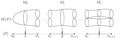
Figure 2. The fibrewise structure of the map $\theta$.

Now, it is clear how we should prove Theorems 13 and 14.

Proof of Theorem 13. We make the following observations. The projection

$$\frac{[a_{i},a_{i+1}]\times\Sigma_{i}}{\sim}\rightarrow[a_{i},a_{i+1}]$$

has sections. Indeed given points $z_{1}$ and $z_{2}$ that lie in the same path component of $\Sigma_{i}$ and given distinct points $x_{1}$ and $x_{2}$ in $[a_{i},a_{i+1}]$ there exists a continuous section

$$\sigma:[a_{i},a_{i+1}]\rightarrow\frac{[a_{i},a_{i+1}]\times\Sigma_{i}}{\sim}$$

such that $\sigma(x_{1})=(x_{1},z_{1})$ and $\sigma(x_{2})=(x_{2},z_{2})$.

By combining $\alpha$ with a judicious use of these sections, it is clear that we can find the required lift of $\alpha$. For the sake of completeness, we have included the details of this argument below. However these details are rather tedious and not particularly enlightening. Thus, if the reader if sufficiently convinced by the arguments already presented, he may, at this point, skip the rest of this proof.

We must consider several different cases. First, let us deal with the case where $p$ and $q$ happen to lie in same fibre of $\theta$. If $\alpha(x)=\theta(p)=\theta(q)$ for all $x\in[0,1]$ then the conclusion is clearly true, as by assumption we must have $\theta(p)\in\nabla(P)$, and therefore we can lift $\alpha$ by choosing a path within $\theta^{-1}(\theta(p))$ that connects $p$ and $q$. If $\alpha$ is not a constant function then we can choose some $b\in[0,1]$ such that $b\neq\theta(p)$ but so that $\alpha([0,b])$ is contained within one of the open intervals $(a_{i},a_{i+1})$. Now it is clear that we can lift $\alpha|_{[0,b]}:[0,b]\rightarrow[P]$ since $\theta$ restricts to a trivial fibre bundle over $\alpha([0,b])$. Thus we are left the problem of lifting $\alpha|_{[b,1]}:[b,1]\rightarrow[P]$ with specified lifts of $b$ and of 1. In other words, we have reduced to case where $p$ and $q$ lie in different fibres of $\theta$.

Suppose now that $p$ and $q$ lie in different fibres of $\theta$. Also suppose that $\theta(p)\in\nabla(P)$ (similar arguments apply if $\theta(q)\in\nabla(P)$). Since we have assumed that $\theta(p)$ is not a critical value, $\theta(p)$ must in fact lie in the interior of $\nabla(P)$. Therefore, by concatenating local sections over $[a_{i},a_{i+1}]$ of the type described above, we can find a (global) section $\gamma:[P]\rightarrow M(P)$ such that $\gamma(\theta(p))=p$ and $\gamma(\theta(q))=q$. Let $\tilde{\alpha}=\gamma\circ\alpha$. Clearly $\tilde{\alpha}$ is the required lift in this case.

Finally, we consider the case where $\theta(p)\notin\nabla(P)$ and $\theta(q)\notin\nabla(P)$. Choose some $c\in[0,1]$ such that $\alpha(c)\in\nabla(P)$ (our hypotheses guarantee the existence of at least one such $c$). Now we choose a point $r$ in the fibre $\theta^{-1}(\alpha(c))$. If $\alpha(c)$ is in the interior of $\nabla(P)$, we can choose $r$ arbitrarily within the fibre. However, if $\alpha(c)$ happens to be on the boundary of $\nabla(P)$ (and is therefore also a critical value of $\theta$), we must be more selective in our choice of $r$. In this case we choose $r$ to a critical point of $\theta$. Now, once we have chosen $r$ in this way, we can find two global sections $\gamma_{1}$ and $\gamma_{2}$ of $\theta$, such that $\gamma_{1}(\alpha(c))=\gamma_{2}(\alpha(c))=r$, $\gamma_{1}(\theta(p))=p$ and $\gamma_{2}(\theta(q))=q$. Now, for $x\in[0,c]$, let $\tilde{\alpha}(x)=\gamma_{1}(\alpha(x))$ and for $x\in[c,1]$, let $\tilde{\alpha}(x)=\gamma_{2}(\alpha(x))$. One readily checks that $\tilde{\alpha}$ is the required lift of $\alpha$ in this case. ∎

Proof of Theorem 14. In the case that one of $p$ or $q$ lies in a critical fibre (i.e the preimage of one of the $a_{i}$s), then it may be necessary to first move to a different point in that fibre to ensure that when we lift along sections, we end up in the right path component of subsequent fibres. The hypotheses of Theorem 14 allow the intervals $[0,\epsilon]$ and $[1-\delta,1]$ to carry out this adjustment within the fibre. ∎

We will also need the following lifting result later. Its proof is again an straightforward consequence of the fibrewise structure of $\theta$ described above, so we shall leave the reader to fill in the details in this case.

Theorem 15.

Let $p\in M(P)$ and suppose that $\alpha:[0,1]\rightarrow[P]$ is a continuous function such that $\alpha(0)=\theta(p)$. There is some continuous lift $\tilde{\alpha}:[0,1]\rightarrow M(P)$ such that $\tilde{\alpha}(0)=p$ and $\theta\circ\tilde{\alpha}=\alpha$.

Now we show that any path in $M(P)$ that connects two different path components of a fibre $\theta^{-1}(x)$ must pass through $\theta^{-1}(\nabla(P))$.

Lemma 16.

Suppose that $x\notin\nabla(P)$ and let $p$ and $q$ be two realisations of $P$ that lie in different components of $\theta^{-1}(x)$. Suppose that $\alpha:[0,1]\rightarrow M(P)$ is a continuous function such that $\alpha(0)=p$ and $\alpha(1)=q$. Then there is some $c\in[0,1]$ such that $\theta(\alpha(c))\in\nabla(P)$.

Proof.

It is clear from the above description of $\theta$ that there must exist $c$ such that $\alpha(c)=a_{j}$ for some critical value $a_{j}$ of $\theta$. However, as remarked above, $a_{j}\in\nabla(P)$. ∎

We conclude this section by observing that if $x\notin\nabla(P)$, if $p\in\theta^{-1}(x)$ and if $\tau$ is any orientation reversing isometry of $\mathbb{R}^{2}$, then $\tau\circ p$ and $p$ lie in different path components of $\theta^{-1}(x)$.

4.2. Determining the connectedness of the moduli space

Now we present a method for checking the connectedness of $M(L)$ when $L=(G,l)$ is a series parallel linkage. First observe that we may as well restrict our attention to the case where the graph $G$ is a 2-connected series parallel graph. If $G$ is not 2-connected, then it can be decomposed into a series composition of 2-connected series parallel graphs. It is clear that $M(L)$ is connected if and only the moduli space of each of the series components of $L$ is connected.

Let $L$ be a 2-connected series parallel linkage such that $M(L)$ is not empty. Recall that, by Lemma 2, we can find vertices $u$ and $v$ such that $(G,u,v)$ is a TTSPG and such that

$$(G,u,v)=(P_{1},u,v)\|(P_{2},u,v)\|\dots\|(P_{n},u,v)\|(K,u,v)$$

where $(K,u,v)$ is a sub TTSPG of $(G,u,v)$ and where each $P_{i}$ is a path joining $u$ and $v$, and $n\geq 2$. See Figure 3 for an illustration of this situation.

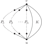
Figure 3.

We will write $L_{K}$ to denote the sublinkage $(K,l|_{K})$ of $L$.

Theorem 17.

With notation as above, if $\nabla(P_{i})\cap[L,u,v]$ is empty for some $i$ then $M(L)$ is disconnected.

Proof.

Let $p\in M(L)$. We can construct another realisation of $L$ by reflecting the vertices $P_{i}$ in a line through $p(u)$ and $p(v)$. Call this realisation $q$. Now if $\alpha:[0,1]\rightarrow M(L)$ is any path, then by assumption $|\alpha(x)(u)-\alpha(x)(v)|\notin\nabla(P_{i})$ for all $x\in[0,1]$. Therefore, by Lemma 16 and the observation that immediately follows that lemma, $\alpha$ cannot be a path that connects $p$ and $q$. ∎

What can we say about the connectedness of $M(L)$ if the hypothesis of Theorem 17 is not satisfied, in other words if $\nabla(P_{i})\cap[L,u,v]$ is non empty for all $i$?

In this case, we construct a path linkage $Q$ as follows. Suppose that $[P_{i}]=[a_{i},b_{i}]$ for $i=1,\dots,n$. Let $a=\max\{a_{i}\}$. Let $b=\min\{b_{i}\}$ (note that $b\geq a$ since $(G,l)$ is realisable). Now let $Q$ be a path linkage with four edges $e_{1},\dots,e_{4}$ and assign length $l_{i}$ to edge $e_{i}$ as follows; $l_{1}=\frac{a+b}{2}$ and $l_{2}=l_{3}=l_{4}=\frac{b-a}{6}$.

Lemma 18.

$[Q]=[a,b]$ and $\nabla(Q)=[a,b]$.

Proof.

The first statement is obvious and the second statement follows immediately from Lemma 11 ∎

Let $s$ and $t$ be the terminal vertices of $Q$ and define a linkage $L_{1}$ by

$$(L_{1},u,v)=(Q,s,t)\|(K_{L},u,v).$$

In other words $L_{1}$ is obtained from $L$ by replacing all the $P_{i}$s by the single path linkage $Q$. Note that $L_{1}$ has a strictly smaller series parallel decomposition in terms of path linkages than $L$ does.

Theorem 19.

With the notation as above, suppose that $\nabla(P_{i})\cap[L,u,v]$ is nonempty for each $i=1,\dots,n$. Then $M(L)$ is connected if and only if $M(L_{1})$ is connected.

Proof.

We first observe that, by construction, $[Q]=[P_{1}]\cap\dots\cap[P_{n}]$. It follows that

$$\text{im}(M(L)\rightarrow M(L_{K}))=\text{im}(M(L_{1})\rightarrow M(L_{K}))$$

where $M(L)\rightarrow M(L_{K})$ and $M(L_{1})\rightarrow M(L_{K})$ are the canonical maps induced by restriction.

Now, suppose that $M(L_{1})$ is connected and let $p$ and $q$ be elements of $M(L)$. We must show that there is a path in $M(L)$ joining $p$ and $q$. We construct this path in several stages. First, by our observations above, we can choose some realisations $p_{1}$ and $q_{1}$ of $L_{1}$ that agree with $p$ and $q$ on $L_{K}$. Now since $M(L_{1})$ is connected, there is some path $\alpha:[0,1]\rightarrow M(L_{1})$ such that $\alpha(0)=p_{1}$ and $\alpha(1)=q_{1}$. Now we can apply Theorem 15 to construct a path $\tilde{\alpha}:[0,1]\rightarrow M(L)$ such that $\tilde{\alpha}(0)=p$ and $\tilde{\alpha}$ agrees with $\alpha$ on vertices of $K$. We just define $\tilde{\alpha}(t)(v)=\alpha(t)(v)$ for all vertices $v\in K$. To lift $\tilde{\alpha}$ to $M(L)$, we use Theorem 15 (once for each $P_{i}$). In particular $\tilde{\alpha}(1)|_{K}=q|_{K}$.

Of course, it may happen that for some or all of the $P_{i}$s, $\tilde{\alpha}(1)|_{P_{i}}\neq q|_{P_{i}}$. So we have to concatenate other paths onto the end of $\tilde{\alpha}$ to “correct” it on the $P_{i}$s. We can do this one $P_{i}$ at as time as follows. Let $x=|q(u)-q(v)|$. By assumption $\nabla(P_{i})\cap[L,u,v]$ is nonempty, so there is some path $\beta:[0,1]\rightarrow[L,u,v]$ such that $\beta(0)=x=\beta(1)$ and such that $\beta(y)\in\nabla(P_{i})$ for some $y\in[0,1]$. Moreover, we can certainly choose $\beta$ so that it is stationary in a neighbourhood of $0$ and in a neighbourhood of $1$. Now, it is clear that by applying Theorem 14 to $\beta$ we can find some $\overline{\beta}:[0,1]\rightarrow M(L)$ such that $\overline{\beta}(0)=\tilde{\alpha}(1)$, $\overline{\beta}(1)|_{P_{i}}=q|_{P_{i}}$ and $\overline{\beta}(1)$ agrees with $\tilde{\alpha}(1)$ for vertices that are not in $P_{i}$. Concatenating $\tilde{\alpha}$ and $\overline{\beta}$ “corrects” the final position of vertices of $P_{i}$. We can repeat this process for all the $P_{i}$s, if necessary, and we eventually end up with the required path in $M(L)$ connecting $p$ and $q$.

The converse can be proved in much the same way. Suppose that $M(L)$ is connected and let $p_{1}$ and $q_{1}$ be points in $M(L_{1})$. We can find $p$ and $q$ in $M(L)$ that agree with $p_{1}$ and $q_{1}$ on $L_{K}$. Since $M(L)$ is connected, we can find a path $\alpha:[0,1]\rightarrow M(L_{K})$ such that $\alpha$ connects $p_{1}|_{L_{K}}$ and $q_{1}|_{L_{K}}$ and such that $\text{im}(\alpha)$ is contained in the image of the natural map $M(L)\rightarrow M(L_{K})$. Now, using Theorem 15, we can lift $\alpha$ to a path $\tilde{\alpha}:[0,1]\rightarrow M(L_{1})$ and using Theorem 14 we can correct $\tilde{\alpha}(1)$ so that it agrees with $q_{1}$ on $Q$ as necessary. Note that Lemma 18 ensures that the hypotheses of Theorem 14 are satisfied in this situation.

∎

Theorems 17 and 19 form the basis of a simple recursive algorithm for deciding whether or not $M(L)$ is connected for a 2-connected series parallel linkage. We informally describe this algorithm by the following sequence of steps. We assume that $M(L)$ is nonempty.

1. Find a parallel decomposition of the form

   $$[L,u,v]=(P_{1},u,v)\|(P_{2},u,v)\|\dots\|(P_{n},u,v)\|(K,u,v)$$

   where $n\geq 2$.

2. Compute $[L,u,v]$ using the methods described in Section 3. Compute $\nabla(P_{i})$ for each $i$ using Lemma 11.

3. If $\nabla(P_{i})\cap[L,u,v]$ is empty for any $i$, then $M(L)$ is not connected and we can stop.

4. If $\nabla(P_{i})\cap[L,u,v]$ is non empty for all $i$, and $K$ is empty then $M(L)$ is connected and we can stop.

5. If $\nabla(P_{i})\cap[L,u,v]$ is non empty for all $i$, and $K$ is non empty then construct the linkage $L_{1}$ as described above and go back to Step (1) with linkage $L_{1}$ as the input.

Example 20.

Let $L$ be the same linkage that we considered in Example 8 and let $P_{1}$, $P_{2}$, $P_{3}$, $P_{4}$ and $P_{5}$ be the sublinkages described earlier. Now observe that

$$(G,c,h)=(P_{2},c,h)\|(P_{3},c,h)\|(((P_{4},a,h)\|(P_{5},a,h))\circ(P_{1},c,a)).$$

It is easy to check (as in Example 8) that

$$[L,c,h]=[3,4]$$

Moreover, $\nabla(P_{2})=\{3,5\}$ and $\nabla(P_{3})=\{0,4\}$. Thus, in this case, the hypotheses of Theorem 19 are satisfied. The linkage $L_{1}$ looks like

Now, one computes that $[L_{1},a,h]=[3,5]$. However, $\nabla(P_{4})=\{1,13\}$ which does not meet $[3,5]$. Therefore, by Theorem 17, $M(L_{1})$ is disconnected. Therefore by Theorem 19, $M(L)$ is disconnected.

Observe that the linkage $L_{1}$ in this example has the property that every polygonal sublinkage has connected moduli space, but that $M(L_{1})$ is disconnected.

4.3. Remarks

We observe that the path lifting results described in Section 4.1 do not in general hold for linkages that are not series parallel. In [McLaughlinThesis], examples are given to demonstrate this. This is one of the reasons why series parallel linkages are easier to understand.

We also remark that it is sometimes possible to adapt our methods to understand linkages that are not series parallel. It may be that a linkage can be series parallel decomposed into smaller linkages, which while not themselves series parallel, are amenable to analysis by other methods. In this case our results may still have some value. Again, see [McLaughlinThesis] for examples.

5. Acknowledgements

We would like to thank Javier Aramayona for many helpful comments and suggestions.