Conformational free energies of methyl-$\alpha$-L-iduronic and methyl-$\beta$-D-glucuronic acids in water.

Abstract

We present a simulation protocol that allows for efficient sampling of the degrees of freedom of a solute in explicit solvent. The protocol involves using a non-equilibrium umbrella sampling method, in this case the recently developed adaptively biased molecular dynamics method, to compute an approximate free energy for the slow modes of the solute in explicit solvent. This approximate free energy is then used to set up a Hamiltonian replica exchange scheme that samples both from biased and unbiased distributions. The final accurate free energy is recovered via the WHAM technique applied to all the replicas, and equilibrium properties of the solute are computed from the unbiased trajectory. We illustrate the approach by applying it to the study of the puckering landscapes of the methyl glycosides of $\alpha$-L-iduronic acid and its C5 epimer $\beta$-D-glucuronic acid in water. Big savings in computational resources are gained in comparison to the standard parallel tempering method.

I Introduction

The field of glycobiology has undergone rapid growth since its name was coined in 1988Rademacher et al. (1988) to refer to the study of the molecular structure and biology of saccharides (or glycans) as they happen in the cell. Linear polysaccharides are ubiquitous in nature. Glycoproteins, proteoglycans and glycolipids are the most common glycoconjugates in mammalian cells (found mainly in the outer cell wall and fluids). In particular, glycosaminoglycans (heparin, heparan sulfate, chondroitin, keratin, dermatan, and many others) comprise a disaccharide unit formed by two aminosugars linked in an alternating fashion with uronic acidsVarki et al. (2009). In this work we consider L-iduronic acid (IdoA), which is the major uronic acid component of the glycosaminoglycans dermatan sulfate and heparinVarki et al. (2009). We also consider its C5 epimer, D-glucuronic acid (GlcA), that dominates in chondroitin and hyaluronan. The IdoA is an uncommon molecule among the pyranoses (carbohydrates whose chemical structure is based upon a six-membered ring of five carbon atoms and one oxygen) because it adopts several conformations, and therefore it is believed to increase the flexibility and conformational freedom of the corresponding polysaccharide chainsFerro et al. (1990).

Computational studies of polysaccharides have evolved along several directions. In particular, considerable work has been devoted to quantum chemical studies of the energetics of relatively small compounds (see, for example, Ref.Rao et al., 1998 and references therein). While very accurate, such ab-initio calculations typically cannot handle explicit solvent over the nanosecond time scale. Yet, it is known that solvation plays a crucial role in the conformational preferences of carbohydratesKirschner and Woods (2001); Almond and Sheehan (2003). Until recently, only coarse-grained models were able to breach the long time scales involved in conformational sampling. However, methodological advances coupled to growing computational power have allowed the realization of all-atom, explicit solvent classical molecular dynamics over hundreds of nanosecondsKräutler et al. (2007). This of course requires the development and improvement of force-fieldsKirschner et al. (2008), which need to be validated by comparison with experiments. Reliable validation necessitates an accurate determination of the properties of the compounds in explicit solventChristen and van Gunsteren (2008), that can be computationally very demanding.

Often, the dynamical aspect of the trajectory generated in the course of a molecular dynamics (MD) simulation is not of interest per se, and the trajectory is used to study an ensemble statistics of some quantities. It was realized long time ago that MD is quite limited when employed for sampling purposes because the trajectory gets trapped in the vicinity of the free energy minima and is very unlikely to cross barriers higher than a few $k_{B}T$. Many approaches to enhance the sampling have been proposed, with different measures of success. It is beyond the scope of this paper to review the different methods (the reader can find a review in Ref.Christen and van Gunsteren, 2008), but we will briefly go over the two methods employed in this work, namely the “replica exchange” methodGeyer (1991) and the adaptively biased molecular dynamics methodBabin et al. (2008).

The idea behind the replica exchange method is to consider several MD trajectories that are generated using different Hamiltonians and exchange those Hamiltonians (or trajectories) in a way that preserves detailed balance so that all the Boltzmann distributions that correspond to the Hamiltonians involved get sampled simultaneously in a mutually enhancing way. The overall performance of the method is determined by the “right” choice of the Hamiltonians involved in the construction. For example, “parallel tempering” (the most popular incarnation of the method) builds the family of Hamiltonians by re-scaling the original Hamiltonian. This is identical to the situation where one Hamiltonian is used at different temperatures – high-temperature replicas have higher barrier-crossing rates and continuously “seed” the low-temperature replicas with different configurations. The advantage of this method is that it is very general requiring little prior knowledge about the system. The disadvantage is that, as the number of degrees of freedom increases, more and more replicas are required to cover the desired range of temperatures while maintaining satisfactory exchange rates. In the pure parallel tempering case, the number of replicas has been shown to grow as the square root of the number of degrees of freedomKofke (2002, 2004).

Over the past few years, several methods targeting the computation of the free energy using non-equilibrium simulations have become popular. These methods all estimate the free energy as a function of “collective variables” from an “evolving” ensemble of realizationsLelièvre et al. (2007); Bussi et al. (2006), and use that estimate to bias the system dynamics, so as to flatten the effective free energy surface. One of the first methods that used the idea of a dynamically evolving potential that forces the system to explore unexplored regions of the phase space was the local elevation methodHuber et al. (1994). More recent developments include the adaptive force bias methodDarve and Pohorille (2001), the Wang-Landau approachWang and Landau (2001), and the non-equilibrium metadynamicsLaio and Parrinello (2002); Iannuzzi et al. (2003) method. Collectively, all these methods may be considered as umbrella sampling methods in which the biasing force compensates for the free energy gradient. In the long time limit, the biasing potential eventually reproduces the previously unknown free energy surface. The adaptively biased molecular dynamics (ABMD) methodBabin et al. (2008) grew out of our efforts to streamline the metadynamics method for classical biomolecular simulationsBabin et al. (2006). It shares all the important characteristics of the above methods while including enhancements in its own right such as a favorable $O(t)$ scaling with time $t$, and a fewer number of control parameters. Adaptive bias methods have been recently used to enhance the conformational sampling of small sugars in explicit water. These efforts include the use of the local elevation method to calculate the relative free energies and interconversion barriers of the ring conformers of $\beta$-D-glucopyranose in waterHansen and Hünenberger (2009), and the use of metadynamics to recover the conformational free energy surface of $\alpha$-N-Acetylneuraminic acidSpiwok and Tvaroška (2009) and $\beta$-D-GlucopyranoseSpiwok et al. (2010). The latter work is an important contribution to the force-field validation process.

It is possible to harness the power of replica exchange with a suitable family of Hamiltonians that are built by biasing the original Hamiltonian along relevant slow modes. These biasing potentials can be readily computed using the adaptive bias methods. In this paper, we combine the ABMD method with the replica exchange and the weighted histogram analysis (WHAMFerrenberg and Swendsen (1989); Kumar et al. (1992)) methods in order to achieve robust sampling of the conformational space of the pyranose ring in explicit solvent, and recover the potential of mean force (free energy) associated with two intra-ring dihedral angles describing the slow puckering modes. The free energy alone could be computed by “correcting” the biasing potential obtained by ABMD with an equilibrium run, as discussed at length in Ref.Babin et al., 2006. The approach explored in this paper replaces the “correction” step with a replica-exchange simulation that both “corrects” the approximate biasing potential and efficiently samples unbiased equilibrium configurations.

Our study has two main goals. First, we present a simulation protocol that allows for efficient sampling of the degrees of freedom of a solute in explicit solvent. Second, we illustrate how this approach can be used to validate the new GLYCAM 06 force fieldKirschner et al. (2008) by means of applying it to the study of the puckering landscapes of the methyl glycosides of $\alpha$-L-iduronic acid and its C5 epimer $\beta$-D-glucuronic acid (see Fig.1).

The paper is organized as follows: the methodology is described in the next section which is followed by the presentation of the simulation protocol along with the results. The paper then ends with a short summary.

II Methods

Let us consider a system of $N$ classical particles. The state of the system can be described by the positions of the particles $\mathbf{r}_{1},\dots,\mathbf{r}_{N}$ and their momenta $\mathbf{p}_{1},\dots,\mathbf{p}_{N}$. Let

$$\mathcal{H}=\sum\limits_{a=1}^{N}\frac{\mathbf{p}^{2}_{a}}{2m_{a}}+\Phi(\mathbf{r}_{1},\dots,\mathbf{r}_{N})$$ (1)

be the Hamiltonian of the system. Here, $m_{a}$ are the masses of the particles and $\Phi(\mathbf{r}_{1},\dots,\mathbf{r}_{N})$ is the potential energy. In the following, we omit the atomic indices if this does not lead to confusion, that is, $\mathbf{r}$ represents $\mathbf{r}_{1},\dots,\mathbf{r}_{N}$ and $\mathbf{p}$ represents $\mathbf{p}_{1},\dots,\mathbf{p}_{N}$.

A routine task in molecular modeling involves sampling configurations according to the canonical distribution

$$\mathcal{P}(\mathbf{p},\mathbf{r})\propto e^{\textstyle-\mathcal{H}(\mathbf{p},\mathbf{r})/k_{B}T}$$ (2)

($k_{B}$ is the Boltzmann constant and $T$ is the temperature). One way of carrying out such sampling is, for instance, to generate dynamics via the Langevin equation such that its limiting probability distribution is the desired equilibrium distributionBrünger et al. (1984). Unfortunately this basic strategy often fails because the system gets either trapped in the neighborhood of a potential energy minimum or locked in some region of phase space due to entropic bottlenecks. Hence, other more elaborate approaches have been proposed throughout the years (see, for example, a review in Ref.Christen and van Gunsteren, 2008). In this paper we describe how a combination of the replica exchangeGeyer (1991), ABMDBabin et al. (2008) and WHAMFerrenberg and Swendsen (1989); Kumar et al. (1992) methods can be used to enhance sampling, and illustrate the use of this protocol by applying it to the study of small solutes in explicit solvent. For clarity and completion, we briefly review these methods below.

II.1 Replica exchange method

The replica exchange ideaGeyer (1991) consists of considering several Hamiltonians, $\mathcal{H}_{a}(\mathbf{p},\mathbf{r})$, $a=1,\dots,M$ (with the original $\mathcal{H}(\mathbf{p},\mathbf{r})$ being of one them), running the dynamics for each of them, and trying to “cross-pollinate” these dynamics by exchanging the trajectories between the different Hamiltonians from time to time. More formally, the method can be implemented as follows: once in a while a random pair of replicas is chosen and an exchange is attempted with the acceptance probability carefully tuned to maintain detailed balance in the extended ensembleGeyer (1991); Sugita et al. (2000)

$$\mathcal{P}_{ab}=\left\{\begin{array}[]{ll}1,&\Delta\leq 0,\\ e^{\textstyle-\Delta},&\Delta>0,\end{array}\right.$$ (3)

$$\Delta = \frac{1}{k_{B}T_{a}}\left[\Phi_{a}(\mathbf{r}^{b})-\Phi_{a}(\mathbf{r}^{a})\right]$$

$$+ \frac{1}{k_{B}T_{b}}\left[\Phi_{b}(\mathbf{r}^{a})-\Phi_{b}(\mathbf{r}^{b})\right],$$

where $T_{a,b}$ denote the temperatures of the replicas and only the potential energy is shown (the momenta are integrated out). In practice, the momenta get simply rescaled upon a successful exchange. In this scheme, high, inaccessible barriers in one replica can be smaller in another replica and hence this random walk over the replicas facilitates barrier crossings. Care must be taken with the choice of Hamiltonians since it determines the performance of the method. There are many variations of replica exchange, with the most popular one being “parallel tempering”: the family of the Hamiltonians is constructed from the rescaled copies of the original one (this is equivalent to having the same Hamiltonian with different temperatures). Parallel tempering has the advantage of being quite general, but the applicability of the method can be limited by the fact that the number of replicas needed to cover a desired temperature range (while maintaining an efficient random walk across those temperatures) grows as the square root of the number of degrees of freedomKofke (2002, 2004).

II.2 Adaptively biased molecular dynamics

The ABMDBabin et al. (2008) method is an umbrella sampling method with a time-dependent biasing potential that can be used to compute the Landau free energy of a collective variable $\sigma(\mathbf{r})$, which is understood to be a smooth function of the atomic positions. The Landau free energy is defined asFrenkel and Smit (2002):

$$f(\xi)=-k_{B}T\ln\big{<}\delta\left[\xi-\sigma(\mathbf{r})\right]\big{>},\;$$

where the angular brackets denote an ensemble average. The free energy $f(\xi)$ (sometimes also referred to as the potential of mean force) describes the relative stability of states corresponding to different values of $\xi$, and can provide insight into the possible transitions between these states.

In the ABMD method an additional time-dependent biasing potential is added to the potential energy of the system

$$\Phi_{{\texttt{ABMD}}}\left(\mathbf{r},t\right)=\Phi\left(\mathbf{r}\right)+U\big{[}\sigma\left(\mathbf{r}\right),t\big{]}.$$

This biasing potential “floods” the true free energy landscape as it evolves in time according to:

$$\frac{\partial U(\xi,t)}{\partial t}=\frac{k_{B}T}{\tau_{F}}G\big{[}\xi-\sigma\left(\mathbf{r}\right)\big{]}.$$

In the last equation $G(\xi)$ denotes the kernel, which is thought to be positive and symmetric (in analogy to the kernel density estimator widely used in statisticsSilverman (1986)). For large enough $\tau_{F}$ (flooding timescale) and small enough kernel width, the biasing potential $U(\xi,t)$ converges towards $-f(\xi)$ as $t\to\infty$Lelièvre et al. (2007); Bussi et al. (2006).

The implementation of the method is straightforward: we use cubic B-splinesDe Boor (1978) (or products of thereof for multidimensional collective variables) to discretize $U(\xi,t)$ in “space”:

$$U(\xi,t)=\sum\limits_{m}U_{m}(t)B(\xi/\Delta\xi-m),$$

$$B(\xi)=\left\{\begin{array}[]{ll}(2-|\xi|)^{3}/6,&1\leq|\xi|<2,\\ \xi^{2}(|\xi|-2)/2+2/3,&0\leq|\xi|<1,\\ 0,&\mathrm{otherwise}.\end{array}\right.$$ (4)

We choose the biweight kernelSilverman (1986) for $G(\xi)$:

$$G(\xi)=\frac{48}{41}\left\{\begin{array}[]{ll}\left(1-\left.\xi^{2}\right/4\right)^{2},&-2\leq\xi\leq 2\\ 0,&\mathrm{otherwise}\end{array}\right.,$$

and Euler-like discretization scheme for the time evolution of the biasing potential:

$$U_{m}(t+\Delta t)=U_{m}(t)+\Delta t\frac{k_{B}T}{\tau_{F}}G\big{[}\sigma/\Delta\xi-m\big{]},$$

where $\sigma=\sigma(\mathbf{r})$ is at time $t$. This discretization in time may readily be improved. However, this is not really important, since the goal is simply to flatten $U(\xi,t)+f(\xi)$ in the long time limit.

II.3 Combination of replica exchange and ABMD

In this paper the ABMD method is used to construct the Hamiltonians for the replica exchange scheme. In particular, we are interested in the properties of a relatively small solute, with a few degrees of freedom, immersed in a much larger “bath” of solvent molecules. Parallel tempering is impractical for such a system due to the large total number of degrees of freedom, requiring many replicas that spend most of the time equilibrating the solvent at different temperatures. On the other hand, especially for small solutes, one can readily identify the slowest modes that are difficult to sample in regular MD on the grounds of physical and/or chemical intuition. Quite often those modes can be described as a motion along a collective variable $\sigma=\sigma(\mathbf{r}_{1},\dots,\mathbf{r}_{S})$ that does not depend on the solvent coordinates explicitly. It is therefore reasonable to consider two (or more – see below) replicas, both running at the same temperature, with the potential energies

$$\Phi_{a}(\mathbf{r})=\Phi(\mathbf{r}),\quad\Phi_{b}(\mathbf{r})=\Phi(\mathbf{r})-f\big{[}\sigma(\mathbf{r}_{1},\dots,\mathbf{r}_{S})\big{]},$$

where the last term in $\Phi_{b}(\mathbf{r})$ is the Landau free energy associated with the collective variable $\sigma$ computed for the original potential energy $\Phi(\mathbf{r})$. This last term renders the states with the different values of the collective variable equally probably in the second replica, which thus plays the role of the high-temperature replicas in the parallel tempering scheme, “speeding” up the motions along the collective variable. The first replica uses the unmodified potential energy, thus producing unbiased samples of the configurations of the original system. Since both replicas run at the same temperature, the exchange probability given in Eq.(3) does not depend explicitly on the potential energy difference between the replicas, but on the biasing potentials as a function of the solute degrees of freedom. Therefore, the necessary number of replicas is expected to be much smaller than it would be for parallel tempering.

The true free energy, $f(\xi)$, is typically unknown in advance. We therefore use the ABMD method to compute a biasing potential $U(\xi)$ that approximately compensates for the unknown free energy $f(\xi)\approx-U(\xi)$ (up to an additive constant). This biasing potential is then used to set up the replica exchange scheme that yields both an enhanced sampling of the solute states and a more accurate Landau free energy $f(\xi)$ associated with $\sigma(\mathbf{r}_{1},\dots,\mathbf{r}_{S})$. The latter is reconstructed using the familiar WHAM approachFerrenberg and Swendsen (1989); Kumar et al. (1992) briefly summarized in the next subsection.

The overall success of the replica exchange scheme is determined by the efficiency of the random walk in the replica space. The latter can be quantified by the exchange rates between the pairs of replicas. Let us consider two replicas running at the same temperature $T$ with the potential energies

$$\Phi_{a,b}(\mathbf{r})=\Phi(\mathbf{r})+U_{a,b}\big{[}\sigma(\mathbf{r}_{1},\dots,\mathbf{r}_{S})\big{]},$$

given by the original potential energy $\Phi(\mathbf{r})$ biased by the potentials $U_{a,b}(\xi)$ acting on the collective variable $\sigma(\mathbf{r}_{1},\dots,\mathbf{r}_{S})$, which is the same in both replicas. The exchange probability Eq.(3) then becomes

$$\mathcal{P}_{ab}=\Theta(\Delta)e^{\textstyle-\Delta}+\Theta(-\Delta),$$

where $\Theta(x)$ is the Heaviside step function,

$$\Delta=\frac{1}{k_{B}T}\big{[}U_{a}(\xi_{b})-U_{a}(\xi_{a})+U_{b}(\xi_{a})-U_{b}(\xi_{b})\big{]},$$

and $\xi_{a,b}$ are the values of the collective variable $\sigma(\mathbf{r}_{1},\dots,\mathbf{r}_{S})$ in the corresponding replicas. The probability densities of the collective variables can be expressed through the associated Landau free energy, $f(\xi)$, computed for the original potential $\Phi(\mathbf{r})$:

$$p_{a,b}(\xi)\propto e^{\textstyle-\big{[}f(\xi)+U_{a,b}(\xi)\big{]}\big{/}k_{B}T},$$

and can readily be used in the expression for the rate of exchange between the two replicas

$$\mathcal{R}_{ab}=\int\!\!\mathrm{d}\xi_{a}\mathrm{d}\xi_{b}\;p_{a}(\xi_{a})p_{b}(\xi_{b})\mathcal{P}_{ab}.$$

The integrals in the above formula are low-dimensional and can easily be computed numerically.

From a practical point of view, the two replicas used in the preceding discussion often render the exchange rate unacceptably low. This can be solved by introducing more replicas, such that the range of biasing potentials goes from zero to the full (approximate) negative free energy through some intermediates. For the present study we chose to use three replicas biased as follows:

$$\Phi_{1}(\mathbf{r})=\Phi(\mathbf{r}),$$

$$\Phi_{2}(\mathbf{r})=\Phi(\mathbf{r})+\lambda U\big{[}\sigma(\mathbf{r}_{1},\dots,\mathbf{r}_{S})\big{]},$$

$$\Phi_{3}(\mathbf{r})=\Phi(\mathbf{r})+\;\;U\big{[}\sigma(\mathbf{r}_{1},\dots,\mathbf{r}_{S})\big{]},$$

where the parameter $\lambda$ is found by imposing equality of exchange rates, $\mathcal{R}_{12}=\mathcal{R}_{23}$. This equation is solved numerically. The resulting exchange rates turned out to be around 30% and were deemed satisfactory. Otherwise, more intermediate replicas would have to be introduced following the same reasoning.

II.4 Weighted histogram analysis method

Here we review the WHAMFerrenberg and Swendsen (1989); Kumar et al. (1992) scheme, following the presentation given in Refs.Bartels and Karplus, 1997; Bartels, 2000; Habeck, 2007. The aim of the WHAM approach is to infer the unbiased free energy out of several biased simulations. More precisely, let us consider $M$ simulations biased by some potentials $U_{m}$, $m=1,\dots,M$ that depend on atomic positions through a collective variable $\sigma(\mathbf{r})$, that is,

$$U_{m}=U_{m}\big{[}\sigma(\mathbf{r}_{1},\dots,\mathbf{r}_{N})\big{]}.$$

Let $K_{m}$ denote the number of values of the collective variable $\sigma$ collected in the $m^{th}$ simulation: $\xi_{m,1},\xi_{m,2},\dots,\xi_{m,K_{m}}$ (with $m=1,\dots,M$). By the end of the simulations, the whole sample $\mathcal{D}$ contains $K_{1}\times K_{2}\times\dots\times K_{M}$ values of the collective variable that are supposed to be statistically independent.

The likelihood to observe a single value of the collective variable in the $m^{th}$ simulation is

$$p(\xi|m)=\frac{1}{\mathcal{Z}_{m}}\int\!\!\mathrm{d}\mathbf{r}\;\delta\big{[}\xi-\sigma(\mathbf{r})\big{]}e^{\textstyle-\beta\Phi_{m}},$$ (5)

where $\beta=1/k_{B}T$, $\Phi_{m}=\Phi+U_{m}$ and

$$\mathcal{Z}_{m}=\int\!\!\mathrm{d}\mathbf{r}\;\mathrm{e}^{\textstyle-\beta\Phi_{m}}.$$

The likelihood (5) can be expressed through the Landau free energy $f(\xi)$ (which is to be determined) associated with the collective variable

$$\mathrm{e}^{\textstyle-\beta f(\xi)}=\frac{1}{\mathcal{Z}}\int\!\!\mathrm{d}\mathbf{r}\;\delta\big{[}\xi-\sigma(\mathbf{r})\big{]}\mathrm{e}^{\textstyle-\beta\Phi},$$

as

$$p(\xi|m)=\mathrm{e}^{\textstyle-\eta_{m}-\beta f_{m}(\xi)},$$

where

$$\mathrm{e}^{\textstyle\eta_{m}}=\frac{\mathcal{Z}_{m}}{\mathcal{Z}}=\int\!\!\mathrm{d}\xi\;\mathrm{e}^{\textstyle-\beta f_{m}(\xi)},$$

$$f_{m}(\xi)=f(\xi)+U_{m}(\xi),$$

and

$$\mathcal{Z}=\int\!\!\mathrm{d}\mathbf{r}\;\mathrm{e}^{\textstyle-\beta\Phi}.$$

The likelihood of the whole dataset $\mathcal{D}$ is

$$L(f|\mathcal{D})=\prod\limits_{m=1}^{M}\prod\limits_{j=1}^{K_{m}}p(\xi_{j,m}|m).$$ (6)

By introducing individual “densities”

$$\Gamma_{m}(\xi)=K_{m}^{-1}\sum\limits_{j=1}^{K_{m}}\delta(\xi-\xi_{j,m}),$$ (7)

one can rewrite the likelihood (6) as follows

$$-\ln L(f|\mathcal{D})=$$ (8)

$$\sum\limits_{m=1}^{M}K_{m} \int\!\!\mathrm{d}\xi\;\Big{[}\eta_{m}+\beta f_{m}(\xi)\Big{]}\Gamma_{m}(\xi).$$

The maximum likelihood principle

$$\frac{\delta}{\delta f(\xi)}L(f|\mathcal{D})=0$$ (9)

then leads to the celebrated WHAM equationsKumar et al. (1992)

$$\mathrm{e}^{\textstyle-\beta f(\xi)}=\frac{\sum\limits_{m=1}^{M}w_{m}\Gamma_{m}(\xi)}{\sum\limits_{m=1}^{M}w_{m}\mathrm{e}^{\textstyle-\eta_{m}-\beta U_{m}(\xi)}},$$ (10)

where

$$w_{m}=\frac{K_{m}}{\sum\limits_{m=1}^{M}K_{m}}.$$

In practiceFerrenberg and Swendsen (1989); Kumar et al. (1992); Roux (1995), people typically use histograms to approximate the densities Eq.(7) and then solve the WHAM equations Eq.(10) to find the weights $\eta_{m}$ iteratively.

Another possibility, which is exploited in this paper, is to maximize the likelihood with respect to the unknown free energy $f(\xi)$ numerically. There are some issues with this approach too. First, the method of maximum likelihood is not very useful if applied directly to the likelihood given by Eq.(8) because the functional is maximized by a sum of delta function spikes at the observationsSilverman (1986). The likelihood should be maximized over a particular class of functions instead. Technically this is typically implemented by adding a penalty term to the likelihoodGood and Gaskins (1971); Silverman (1982). While theoretically interesting, in this paper we overcome the problem in a similar way that WHAM does: by smoothening the “densities” (7). Unlike the classical WHAM papers, where the densities are approximated by piece-wise constants (histograms), we use the so-called kernel density estimator for the biased densities (7). That is, we replace $\Gamma_{m}(\xi)$ by $\widetilde{\Gamma}_{m}(\xi)$ which is obtained from the former by using Gaussian kernels

$$\mathcal{G}(\xi)=\frac{1}{h\sqrt{2\pi}}\exp\left[-\frac{1}{2}\xi^{2}/h^{2}\right]$$ (11)

in place of the $\delta$-functions.

Another issue with the functional (8) is that it is invariant with respect to the shifts of the free energy $f(\xi)$ by a constant. While perfectly physical, this feature needs special attention in a numerical setting and hence it is desirable to get rid of it before hand. To this end, we consider the following functionalSilverman (1986, 1982) in place of the original one:

$$\widetilde{L} =\mathrm{e}^{\textstyle w_{1}\eta_{1}+\dots+w_{M}\eta_{M}}$$ (12)

$$+ \beta\sum\limits_{m=1}^{M}w_{m}\int\!\!d\xi f(\xi)\Gamma_{m}(\xi).$$

It is easy to see that the unconstrained minimum of the $\widetilde{L}$ functional coincides with a constrained maximum of the original likelihood (8). The functional (12) is thus much more convenient for numerical treatment since the constrained optimization problem gets reduced to an unconstrained one.

Figure 1: Structure of the methyl glycosides of $\alpha$-L-iduronic acid (IdoA, left) and its C5 epimer $\beta$-D-glucuronic acid (GlcA, right).

Technically, we represent the unknown free energy $f(\xi)$ in the cubic $B$-splinesDe Boor (1978) basis, just as we do with the biasing potential $U(\xi)$. The functional $\widetilde{L}$ then becomes a function of the coefficients. Finally, we minimize this function to find the unknown coefficients numerically using the L-BFGS algorithmNocedal (1980); Liu and Nocedal (1989).

III $\alpha$-L-iduronic and $\beta$-D-glucuronic methyl glycosides

Figure 2: Ring carbon atom numbering (ring oxygen atom O5 is the atom number zero) and some conformers of the pyranoid ring: ${}^{4}C_{1}$, ${}^{2}S_{0}$, ${}^{1}C_{4}$ and ${}^{1}S_{3}$ (from left to right).

We consider methyl glycosides of the $\alpha$-L-iduronic acid (IdoA), the major uronic acid component of the glycosaminoglycans dermatan sulfate and heparinVarki et al. (2009), and its C5 epimer, $\beta$-D-glucuronic acid, predominant in heparan sulfate (Fig.1). The IdoA residue is special among pyranoses because it can adopt several conformations, thus giving flexibility and conformational freedom to the corresponding polysaccharide chainsFerro et al. (1990). We concentrate on the conformational sampling of these molecules as parameterized by the GLYCAM 06Kirschner et al. (2008) force-field in explicit TIP3PJorgensen et al. (1983) water.

There are fourteen “canonical” puckering states of the pyranose ring that minimize the angle strain: two chairs, six boats and six skew-boats (see Ref.Stoddart, 1971 for a more comprehensive presentation). The ${}^{4}C_{1}$ and ${}^{1}C_{4}$ chair conformations, the ${}^{2}S_{0}$ and ${}^{1}S_{3}$ skew-boats, and the nomenclature for the ring carbon atoms, are sketched in Fig.2. The puckering states are named with a $C$, $B$ or $S$ letter for chair, boat or skew-boat respectively. The letter is then superscripted/subscripted with the number(s) of the atom(s) above/below the reference plane (the superscripts are placed in front of the letter while the subscripts go after it). The reference plane is chosen to contain four of the ring atoms and if ambiguity occurs (in the chair and skew-boat conformers), the plane is chosen so that the lowest numbered carbon atom is out of this plane.

For the majority of pyranoses, the ${}^{4}C_{1}$ chair conformation is the only relevant one with the others being much higher in energy. The IdoA is an exception for which both ${}^{4}C_{1}$ and ${}^{1}C_{4}$ chairs have been observedFerro et al. (1990) along with the ${}^{2}S_{0}$ skew-boat. Given the special place of the iduronic acid among the rest of the pyranoses, it is important to be able to accurately reproduce its conformational equilibrium in molecular dynamics simulations. However, the barriers separating the two chair conformations are of order of at least $\approx 10k_{B}T$Forster and Mulloy (1993); Kräutler et al. (2007), and thus the corresponding transitions are rather unlikely on the 10-100 nanosecond timescale. In particular, in Ref.Forster and Mulloy, 1993, the authors conclude: “The frequency of ring conformation interchange … is too slow to allow the accurate prediction of the proportion of each form from molecular dynamics alone”. The combination of the methods described in the preceding section allows us to overcome this difficulty.

IV Results

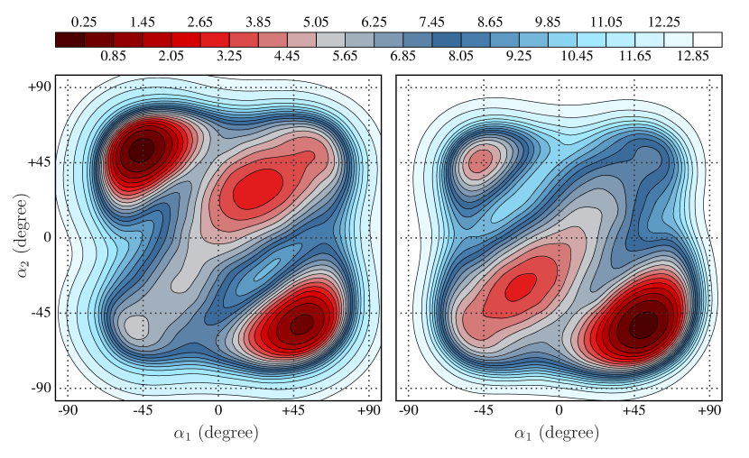
Figure 3: Free energies (kcal/mol) associated with the O5–C1–C2–C3 ($\alpha_{1}$) and C3–C4–C5–O5 ($\alpha_{2}$) dihedral angles for the IdoA (left) and GlcA (right) methyl glycosides (shown in Fig.1) in aqueous solution (TIP3P water).

We use the intra-ring O5–C1–C2–C3 and C3–C4–C5–O5 torsion angles (denoted $\alpha_{1}$ and $\alpha_{2}$ in the following) to distinguish among the different conformations. Our choice is not unique, but this is of minor importance since the dihedrals adopt distinctly different values for the conformations in question: the values of the angles are of different sign for the chairs (with ${}^{1}C_{4}$ corresponding to $\alpha_{1}\approx-50^{\circ}$, $\alpha_{2}\approx+50^{\circ}$ and ${}^{4}C_{1}$ having $\alpha_{1}\approx+50^{\circ}$, $\alpha_{2}\approx-50^{\circ}$) and of the same sign for the boats and skew-boat conformations.

Our goal is to sample the equilibrium configurations of the rings in the NTV ensemble using explicit solvent. We proceed in stages as follows: (1) compute with ABMD an approximate free energy for the dihedral angles using a relatively cheap and fast implicit solvent model; (2) introduce explicit solvent and “refine” the potential of mean force (PMF) from the previous step; (3) set up a replica exchange scheme that uses the approximate PMF to sample from an unbiased canonical distribution while collecting the biased samples as well. The trajectories from the last step are then used to study equilibrium properties of the rings and to recover the accurate free energies using the WHAM technique. The general philosophy behind the protocol is to start with coarser, considerably cheaper approximations that are successively refined with more accurate, expensive approaches such that the final results have the accuracy of the expensive approach at a fraction of the cost. Thus we start with implicit solvent and then use these results as the starting point for explicit solvent.

Let us describe the simulation protocol step by step. The simulation technical details can be found in Appendix A.

IV.1 Step 1: flooding with implicit water

We start sampling in implicit water. A short run at $T=300K$ revealed that the angles fluctuate with an amplitude of $\approx 10$ degrees and a characteristic time (taken to be the period of oscillations here) of 0.5ps. We thus performed a flooding ABMD run with $4\Delta\xi=17^{\circ}$ (for both torsional angles) and $\tau_{F}=1\mathrm{ps}$. We monitored the trajectory and continued running until both angles visited all the values between $\approx-80^{\circ}$ and $\approx+80^{\circ}$ (that is, until the minima corresponding to both the ${}^{4}C_{1}$ and ${}^{1}C_{1}$ chair conformations and skew-boat configurations were “flooded”). The coarse stage took 1ns. We then decreased the spatial resolution to $4\Delta\xi=11^{\circ}$ and increased the timescale to $\tau_{F}=50\mathrm{ps}$ and continued the flooding to refine the biasing potential obtained in the previous step. It took 3ns more of simulation time to cover the desired values of $\alpha_{1,2}$. The biasing potential at this stage is expected to provide a relatively good approximation of the corresponding free energy. (It is not necessary to compute the error at this stage since this potential is only an approximation to be used in the next step).

Regarding the choice of the “spatial” resolution $4\Delta\xi$, we have to balance two conflicting factors: a smaller resolution allows the identification of the finer details of the free energy; yet for a smaller $4\Delta\xi$ (and fixed flooding rate $\tau_{F}$), the accuracy of the free energy decreases because the system experiences stronger biasing forces pushing it out of the thermodynamic equilibrium. We thus choose the resolution to be sufficiently small to approximate the equilibrium minima well.

IV.2 Step 2: flooding with explicit water

It is reasonable to expect that the biasing potential obtained with implicit solvent provides a good approximation for the free energy in explicit solvent. To account for the differences between the two solvent descriptions, we carried out more flooding in explicit solvent with $\tau_{F}=50\mathrm{ps}$ and $4\Delta\xi=11^{\circ}$ (i.e., the “fine” values used for the implicit solvent simulation). After just 5ns, every value of the angles was visited and so we stopped the flooding. Next, we performed a 5ns equilibrium MD run biased by the biasing potential computed so far. The biased trajectory visited all the values in the interval $-80^{\circ}\leq\alpha_{1,2}\leq+80^{\circ}$. This means that the biasing potential approximates the true free energy surface to within a few $k_{B}T$ (otherwise the trajectory would get trapped somewhere; the fact that $\alpha_{1,2}$ sweep the whole region implies that the error is of order of a few $k_{B}T$ at most).

IV.3 Step 3: replica exchange with explicit water

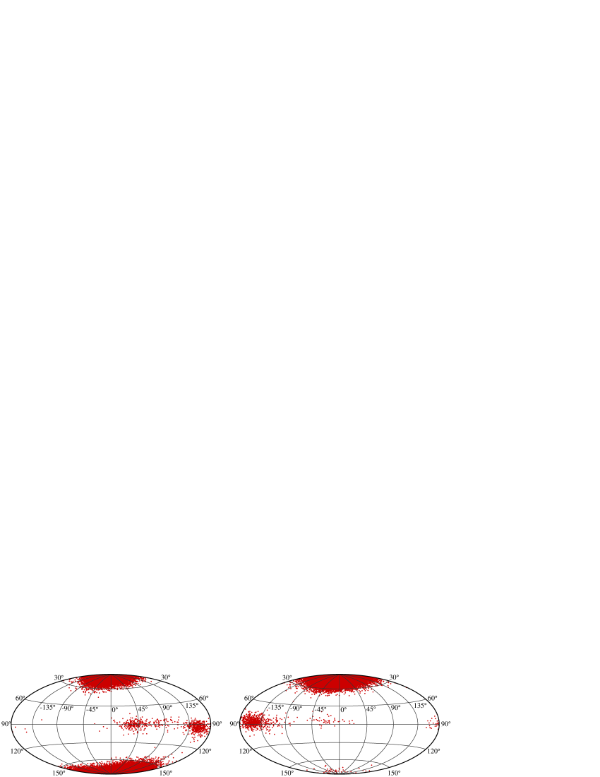
Figure 4: The $(\vartheta,\varphi)$ angles of pseudo-rotationCremer and Pople (1975) for the IdoA (left) and GlcA (right) methyl glycosides in aqueous solution (TIP3P water) at $T=300$K (using the Hammer-AitoffSnyder (1997) equal-area projection).

Finally, we set up a replica exchange scheme that samples both biased and unbiased configurations. This allows for: (a) the computation of the accurate free energy associated with the ring puckering states, and (b) the computation of the unbiased equilibrium averages, such as $J$-couplings, which are of particular interest since they allow for a direct comparison with the NMR data. This last aspect is of paramount importance for the force-field development.

As we described in the “Methods” section, we put three replicas together: the first replica is not biased, the second one is biased by $\lambda U(\xi)$, and the third one is biased by the full $U(\xi)$. We determined the value of $\lambda=0.7$ numerically solving the equation $\mathcal{R}_{12}=\mathcal{R}_{23}$. After a short 1ns equilibration, we went into “production runs” for 100ns trying to exchange a random pair of replicas every 1ps. The observed exchange rates of $\approx 30\%$ were in perfect agreement with the expected values (computed assuming that $f(\xi)=-U(\xi)$) for both IdoA and GlcA cases.

We emphasize that the simulations in explicit solvent involve jumps over barriers of order of 6.5kcal/mol ($\approx 10k_{B}T$). In order for conventional parallel tempering to be able to sample this system, the highest temperature replica would have to run at $\approx 10\times 300K$. This is a prohibitively large number since several hundreds replicas running at intermediate temperatures would be needed to proxy between the highest and the lowest (room) temperatures.

IV.4 Accurate free energies using WHAM

Since the autocorrelation time for the angles in a fully biased MD run is approximately 10ps, we regarded the samples taken 10ps apart during the equilibrium replica exchange as statistically “independent”. Therefore we saved the coordinates from the unbiased replica every 10ps to compute various equilibrium properties of the IdoA and GlcA, reported in the subsection below. We used the whole sample from all three replicas and the WHAM scheme to recover the accurate free energy, shown in Fig.3.

A crucial part of this step is the selection of the kernel bandwidth $h$ in Eq.(11). Assuming that the data is statistically independent, we computed optimal $h$ by minimizing the least-squares cross-validation score to get $h\approx 1.1^{\circ}$ for all the runs; we also computed the bandwidths by maximizing the likelihood cross-validation score getting $h\approx 2.9^{\circ}$ for all the runs. The values selected by both methods were checked using the Silverman’s “visual” method and appeared to be too small (a problem described, for example, in Ref.Loader, 1999). Combining all the hints we chose $h=5.73^{\circ},\;8.59^{\circ}\;\mathrm{and}\;11.46^{\circ}$ for the unbiased, intermediate and fully biased replicas, respectively.

IV.5 Equilibrium properties of the compounds

We computed the Cremer-Pople puckering parametersCremer and Pople (1975) regarding the O5 oxygen as the ring apex (atom number one in the Cremer-Pople formulae) and the carbon with the glycosidic linkage (C1) as the atom number two. The mean value of the puckering amplitude $Q$ turned out to be 0.53Å and 0.55Å (for IdoA and GlcA respectively) with standard deviation $\approx 0.04$Å for both compounds. Both $\vartheta$ and $\varphi$ pseudo-rotation angles display somewhat larger variations and hence are shown in Fig.4 using the Hammer-AitoffSnyder (1997) equal-area projection:

$$(\vartheta,\varphi)\to\left(\frac{2\sqrt{2}\sin\vartheta\sin\varphi/2}{\sqrt{1+\sin\vartheta\cos\varphi/2}},\frac{\sqrt{2}\cos\vartheta}{\sqrt{1+\sin\vartheta\cos\varphi/2}}\right).$$

The $(\vartheta,\varphi)$ values are consistent with the free energies associated with the $\alpha_{1,2}$ (see Fig.3): there are two well-pronounced clusters near the poles for IdoA corresponding to the ${}^{4}C_{1}$ (north pole, $\vartheta=0^{\circ}$) and ${}^{1}C_{4}$ (south pole, $\vartheta=180^{\circ}$) chair conformations, and just one big cluster near the north pole (${}^{4}C_{1}$ chair) for the GlcA. The boat and twisted boat conformations correspond to the equatorial area ($\vartheta=0^{\circ}$) and are indeed considerably less frequent than the chairs. For IdoA the majority of the “equatorial” samples is around $\varphi=150^{\circ}$ (${}^{2}S_{0}$ skew-boat), yet several other twisted boat conformations are also present. This is in accord with Ref.Ernst et al., 1998 where it has been suggested that not only “canonical” boat and skew-boat conformations, but also various boat-like intermediates, contribute to the conformational equilibrium. The most frequent skew-boat conformation for GlcA observed to be ${}^{1}S_{3}$ ($\varphi$ around $-150^{\circ}$).

In order to identify the pyranose puckering states explored during the simulations, one has to choose a criterion for assigning a particular trajectory section to a canonical puckering state. When the temperature is zero, the potential energy minima typically define the conformations in a unique and natural way. At non-zero temperature, however, some ambiguity is always present due to the thermal fluctuations. In our simulations, the ${}^{4}C_{1}$ and ${}^{1}C_{4}$ chair conformations are clearly discriminated by the signs of the $\alpha_{1,2}$ angles and hence we assume that the equilibrium samples with $(\alpha_{1}>0,\alpha_{2}<0)$ are ${}^{4}C_{1}$ chairs while those with $(\alpha_{1}<0,\alpha_{2}>0)$ are ${}^{1}C_{4}$ chairs. The boat and skew-boat conformations, on the other hand, correspond to angles of the same sign, yet it is difficult to distinguish among the different boat and skew-boat types using the $\alpha_{1,2}$ angles alone. The Cremer-Pople parameters could potentially discriminate among the boats, but the ambiguity still persists as one would have to set the boundaries between the conformations. Thus, in the following we concentrate on the properties of the chair conformations, although our simulations show that different skew-boat conformations show up at the thermodynamic equilibrium. In the case of IdoA the majority of those are ${}^{2}S_{0}$-like (left panel in Fig.4: dots in the equatorial area with $\varphi$ around $150^{\circ}$) and ${}^{3}S_{1}$-like ($\varphi$ around $30^{\circ}$). This is in agreement with the conclusions of Mulloy and ForsterMulloy and Forster (2000) that the ${}^{4}C_{1}\leftrightarrow^{1}C_{4}$ transformation of IdoA proceeds through the ${}^{2}S_{0}$ and ${}^{3}S_{1}$ intermediates.

We were able to compute the free energy differences between the ${}^{4}C_{1}$ and ${}^{1}C_{4}$ states by counting the number of configurations $\mathcal{N}(\alpha_{1},\alpha_{2})$ with the appropriate signs of the $\alpha_{1,2}$ angles:

$$\Delta G^{\circ} =-k_{B}T\ln\frac{p(^{4}C_{1})}{p(^{1}C_{4})}$$

$$\approx-k_{B}T\ln\frac{\mathcal{N}(\alpha_{1}>0,\alpha_{2}<0)}{\mathcal{N}(\alpha_{1}<0,\alpha_{2}>0)},$$

where $p(^{4}C_{1})$ and $p(^{1}C_{4})$ denote the probabilities of the corresponding conformations. We obtained

$$\Delta G^{\circ}_{\mathrm{IdoA}}=0.71\mathrm{kcal/mol},\;\Delta G^{\circ}_{\mathrm{GlcA}}=-4.49\mathrm{kcal/mol}.$$

In other words, ${}^{1}C_{4}$ turns out to be marginally more stable than ${}^{4}C_{1}$ for IdoA, while for GlcA, ${}^{4}C_{1}$ is considerably more stable than ${}^{1}C_{4}$. The preference of ${}^{1}C_{4}$ over ${}^{4}C_{1}$ for IdoA appears to be largely due to solvation effects – the vacuum energies optimized in the GLYCAM 06 force-field differ merely by 0.2kcal/mol. On the other hand, the ${}^{4}C_{1}$ has much lower energy than ${}^{1}C_{4}$ for the GlcA in the gas phase and thus the ${}^{4}C_{1}$ stability in water is more due to the “internal” energetics than to solvent interactions or temperature.

	IdoA		GlcA
	${}^{4}C_{1}$	${}^{1}C_{4}$	${}^{4}C_{1}$
Bond angle
C5–O5–C1	116.7(3.3)	116.6(3.3)	116.0(3.5)
O5–C1–C2	110.0(3.0)	111.4(2.8)	109.7(3.0)
C1–C2–C3	111.6(3.2)	112.8(2.8)	112.1(3.2)
C2–C3–C4	113.4(3.2)	114.2(3.0)	112.6(3.2)
C3–C4–C5	112.4(3.0)	111.6(2.9)	112.8(3.2)
C4–C5–O5	107.9(2.8)	109.5(2.8)	108.3(2.9)
Dihedral angle
C5–O5–C1–C2	-57.9(6.7)	53.4(6.4)	-58.2(7.4)
O5–C1–C2–C3	49.3(7.3)	-45.6(6.2)	50.2(7.4)
C1–C2–C3–C4	-47.2(7.3)	45.3(6.3)	-47.1(7.3)
C2–C3–C4–C5	49.4(6.6)	-49.0(5.9)	48.8(6.9)
C3–C4–C5–O5	-51.8(6.0)	52.2(5.6)	-52.0(6.7)
C4–C5–O5–C1	58.7(6.1)	-56.9(6.3)	58.9(7.3)

Table 1: Mean value and standard deviation (in parenthesis) of the intra-ring bond and dihedral angles for IdoA and GlcA methyl glycosides in ${}^{4}C_{1}$ and ${}^{1}C_{4}$ conformations (degrees).

Finally, in order to make connection with NMR spectral dataFerro et al. (1990), we computed the J-couplings for these molecules. Also known as indirect dipole-dipole coupling, a J-coupling is the coupling between two nuclear spins caused by bonding electrons acting on the magnetic field through the two nuclei. J-couplings can be linked to the dihedral angles via the Karplus equationKarplus (1963):

$$^{3}J_{HH}=A\cos^{2}\varphi+B\cos\varphi+C,$$ (13)

We used the values of the parameters reported in Ref.Haasnoot et al., 1980. The ${}^{3}J_{HH}$-coupling constants are presented in Fig.5. We have carried out a considerably accurate sampling of phase space for these molecules, but naturally the validity of the final numbers depend on the validity of the force-field and is also limited by the accuracy of the Karplus equation Eq.(13). The distribution of the ${}^{3}J_{HH}$ values for IdoA clearly reflects the contributions from the two chair conformations, yet the mean values do not match the ones reported in Ref.Ferro et al., 1990 exactly. Specifically, the mean values of the ${}^{3}J_{HH}$ for the methyl-$\alpha$-L-Iduronic acid reported in Ref.Ferro et al., 1990 (line 1, Table I in that reference) are $J_{1,2}=4.9$, $J_{2,3}=6.6$, $J_{3,4}=6.0$ and $J_{4,5}=4.0$ Hz implying that ${}^{4}C_{1}$ is favored over ${}^{1}C_{4}$ contrary to our results. We also note that, due to the bimodal nature of the IdoA’s ${}^{3}J_{HH}$ distributions (see Fig.5), the discrepancies of the mean values can be deceptive. Unfortunately, while there are ample experimental data on oligo- and polysaccharides, information about their monosaccharide units is sketchy and scattered across the scientific literatureKräutler et al. (2007), which prevents more rigorous comparisons.

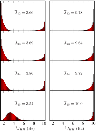
Figure 5: Distributions of the H-H coupling constants computed using the Karplus equation for IdoA (left) and GlcA (right). Mean value shown in the insets.

V Summary

In this work we carried out simulations of methyl-$\alpha$-L-iduronic and methyl-$\beta$-D-glucuronic acids parametrized by the GLYCAM 06 force field in explicit TIP3P water. The importance of these small sugars is greatly due to the fact that IdoA is the major uronic acid component of the glycosaminoglycans dermatan sulfate and heparin, while GlcA dominates in heparan sulfate. The main purpose of this work was to introduce a procedure that reliably recovers the free energy of the solvated molecules and samples the solute degrees of freedom in explicit solvent using very moderate computational resources.

Succinctly, the protocol involves the following steps: (i) use ABMD to compute an approximate free energy for the intra-ring dihedral angles in a relatively cheap implicit solvent; (ii) refine the free energy with ABMD under explicit solvent; (iii) use this last free energy to set up a Hamiltonian replica exchange scheme that samples both from biased and unbiased distributions; and (iv) recover the accurate free energies via the WHAM technique applied to all the replicas, and compute equilibrium properties of the rings from the unbiased trajectories.

The protocol appears to be slightly more complex than the standard parallel tempering method. However, big savings in computational resources fully compensate for this extra “complication”. The simulations in explicit solvent reported in this paper involve jumps over barriers of order of $\approx 10k_{B}T$. An efficient parallel tempering setup in this case would have to run the highest temperature replica at $\approx 10\times 300K$. This rather high temperature would in turn require several hundred replicas to mediate between this highest and the room temperature. In our scheme all replicas run at the same temperature, and hence the exchange probability given in Eq.(3) does not depend explicitly on the potential energy difference between the replicas; it depends, instead, on the differences of the biasing potentials, which are functions of the solute degrees of freedom only. Therefore, the necessary number of replicas is considerably smaller (three replicas were enough for the pyranose rings considered in this paper).

Once that accurate sampling is not an issue anymore, one can really concentrate on problems associated with the validity of the force-field representation. In particular, one can compare against experimentally measurable quantities, such as $J$-couplings, with the certitude that any deviations from experimental values are due to inaccuracies of the force-field (of course, assuming that the experimental values are correct). Naturally, one can extend this study to take into account the effects of different densities, salt concentrations, temperature, etc.

Appendix A Simulation details.

The simulations presented in this paper were performed using the AMBER 10Case et al. (2008) simulation package. The LEaP program from that package was used to prepare the initial structures along with the topology/parameter files. The GLYCAM 06Kirschner et al. (2008) force field was used for the solutes.

The implicit solvent simulations were carried out using the generalized Born modelOnufriev et al. (2000, 2004), including surface area contribution computed using the LCPO modelWeiser et al. (1999) with the surface tension set to $5\times 10^{-3}$ kcal/mol/Ų. The GB/SA simulations were performed enforcing no cutoff on the non-bonded (van der Waals and electrostatics) interactions.

The TIP3P water modelJorgensen et al. (1983) was used for the explicit solvent simulations (in each case 645 water molecules were added along with a $\mathrm{Na}^{+}$ ion to neutralize the system). For the explicit water simulations, we used periodic boundary conditions with fixed box size (27Å in all three directions) chosen to render the density equal to $\approx 1\mathrm{g}/\mathrm{cm}^{3}$. The Particle Mesh Ewald (PME)Darden et al. (1993); Essmann et al. (1995) method was used with the direct space cutoff set to 9Å and a $32\times 32\times 32$ grid for the smooth part of the Ewald sum.

The lengths of all bonds that contain hydrogen were fixed via the SHAKE algorithm with the tolerance set to $10^{-6}$Å. Langevin dynamicsBrünger et al. (1984) with collision frequency $\gamma=1\mathrm{ps}^{-1}$ was used to keep the temperature at 300K. A different random number generator seed was set for every run.

References

- Rademacher et al. (1988) T. W. Rademacher, R. B. Parekh, and R. A. Dwek, Annu. Rev. Biochem. 57, 785 (1988).
- Varki et al. (2009) A. Varki, R. Cummings, J. Esko, H. Freeze, G. Hart, and J. Marth, eds., Essentials of Glycobiology (Cold Spring Harbor Laboratory Press, New York, 2009).
- Ferro et al. (1990) D. R. Ferro, A. Provasoli, M. Ragazzi, B. Casu, G. Torri, V. Bossennec, B. Perly, P. Sinaÿ, M. Petitou, and J. Choay, Carbohydrate Research 195, 157 (1990).
- Rao et al. (1998) V. S. R. Rao, P. K. Qasba, P. V. Balaji, and R. Chandrasekaran, Conformation of Carbohydrates (Harwood Academic Publishers, Amsterdam, 1998).
- Kirschner and Woods (2001) K. N. Kirschner and R. J. Woods, Proc. Natl. Acad. Sci. 98, 10541 (2001).
- Almond and Sheehan (2003) A. Almond and J. K. Sheehan, Glycobiology 13, 255 (2003).
- Kräutler et al. (2007) V. Kräutler, M. Müller, and P. H. Hünenberger, Carbohydrate Research 342, 2097 (2007).
- Kirschner et al. (2008) K. N. Kirschner, A. B. Yongye, S. M. Tschampel, J. González-Outeiriño, C. R. Daniels, B. L. Foley, and R. J. Woods, J. Comp. Chem. 29, 622 (2008).
- Christen and van Gunsteren (2008) M. Christen and W. F. van Gunsteren, J. Comp. Chem. 29, 157 (2008).
- Geyer (1991) C. J. Geyer, in Computing Science and Statistics: The 23rd symposium on the interface (Interface Foundation, Fairfax, 1991), pp. 156 – 163.
- Babin et al. (2008) V. Babin, C. Roland, and C. Sagui, J. Chem. Phys. 128, 134101 (pages 7) (2008).
- Kofke (2002) D. A. Kofke, J. Chem. Phys. 117, 6911 (2002).
- Kofke (2004) D. A. Kofke, J. Chem. Phys. 120, 10852 (2004).
- Lelièvre et al. (2007) T. Lelièvre, M. Rousset, and G. Stoltz, J. Chem. Phys. 126, 134111 (2007).
- Bussi et al. (2006) G. Bussi, A. Laio, and M. Parrinello, Phys. Rev. Lett. 96, 090601 (2006).
- Huber et al. (1994) T. Huber, A. E. Torda, and W. F. van Gunsteren, J. Comput. Aided. Mol. Des. 8, 695 (1994).
- Darve and Pohorille (2001) E. Darve and A. Pohorille, J. Chem. Phys. 115, 9169 (2001).
- Wang and Landau (2001) F. Wang and D. P. Landau, Phys. Rev. Lett. 115, 2050 (2001).
- Laio and Parrinello (2002) A. Laio and M. Parrinello, Proc. Natl. Acad. Sci. 99, 12562 (2002).
- Iannuzzi et al. (2003) M. Iannuzzi, A. Laio, and M. Parrinello, Phys. Rev. Lett. 90, 238302 (2003).
- Babin et al. (2006) V. Babin, C. Roland, T. A. Darden, and C. Sagui, J. Chem. Phys. 125, 204909 (2006).
- Hansen and Hünenberger (2009) H. S. Hansen and P. H. Hünenberger, J. Comp. Chem. 9999, e (2009).
- Spiwok and Tvaroška (2009) V. Spiwok and I. Tvaroška, J. Phys. Chem. B 113, 9589 (2009).
- Spiwok et al. (2010) V. Spiwok, B. Králov,́ and I. Tvaroška, Carbohydrate Research 345, 530 (2010).
- Ferrenberg and Swendsen (1989) A. M. Ferrenberg and R. H. Swendsen, Phys. Rev. Lett. 63, 1195 (1989).
- Kumar et al. (1992) S. Kumar, J. M. Rosenberg, D. Bouzida, R. H. Swendsen, and P. A. Kollman, J. Comp. Chem. 13, 1011 (1992).
- Brünger et al. (1984) A. Brünger, C. L. Brooks, and M. Karplus, Chem. Phys. Lett. 105, 495 (1984), ISSN 0009-2614.
- Sugita et al. (2000) Y. Sugita, A. Kitao, and Y. Okamoto, J. Chem. Phys. 113, 6042 (2000).
- Frenkel and Smit (2002) D. Frenkel and B. Smit, Understanding Molecular Simulation, Computational Science Series (Academic Press, 2002).
- Silverman (1986) B. W. Silverman, Density Estimation for Statistics and Data Analysis, Monographs on statistics and applied probability (Chapman and Hall, 1986).
- De Boor (1978) C. De Boor, A practical guide to splines (Springer-Verlag, New York, 1978), ISBN 0387903569 3540903569 0387903569 3540903569.
- Bartels and Karplus (1997) C. Bartels and M. Karplus, J. Comp. Chem. 18, 1450 (1997).
- Bartels (2000) C. Bartels, Chem. Phys. Lett. 331, 446 (2000).
- Habeck (2007) M. Habeck, Phys. Rev. Lett. 98, 200601 (pages 4) (2007).
- Roux (1995) B. Roux, Computer Physics Communications 91, 275 (1995).
- Good and Gaskins (1971) I. J. Good and R. A. Gaskins, Biometrika 58, 255 (1971).
- Silverman (1982) B. W. Silverman, Annals of Statistics 10, 795 (1982).
- Nocedal (1980) J. Nocedal, Mathematics of Computation 35, 773 (1980).
- Liu and Nocedal (1989) D. C. Liu and J. Nocedal, Math. Program. 45, 503 (1989).
- Jorgensen et al. (1983) W. L. Jorgensen, J. Chandrasekhar, J. Madura, and M. L. Klein, J. Chem. Phys. 79, 926 (1983).
- Stoddart (1971) J. F. Stoddart, Stereochemistry of Carbohydrates (John Wiley & Sons Inc, 1971).
- Forster and Mulloy (1993) M. J. Forster and B. Mulloy, Biopolymers 33, 575 (1993).
- Cremer and Pople (1975) D. Cremer and J. A. Pople, J. Am. Chem. Soc. 97, 1354 (1975).
- Snyder (1997) J. P. Snyder, Flattening the earth : two thousand years of map projections (University of Chicago Press, Chicago, 1997).
- Loader (1999) C. R. Loader, Annals of Statistics 27, 415 (1999).
- Ernst et al. (1998) S. Ernst, G. Venkataraman, V. Sasisekharan, R. Langer, C. L. Cooney, and R. Sasisekharan, J. Am. Chem. Soc. 120, 2099 (1998).
- Mulloy and Forster (2000) B. Mulloy and M. J. Forster, Glycobiology 10, 1147 (2000).
- Karplus (1963) M. Karplus, J. Am. Chem. Soc. 85, 2870 (1963).
- Haasnoot et al. (1980) C. A. G. Haasnoot, F. A. A. M. de Leeuw, and C. Altona, Tetrahedron 36, 2783 (1980).
- Case et al. (2008) D. Case, T. Darden, T. Cheatham, III, C. Simmerling, J. Wang, R. Duke, R. Luo, M. Crowley, R. andW. Zhang, et al., AMBER 10 (University of California, San Francisco, 2008).
- Onufriev et al. (2000) A. Onufriev, D. Bashford, and D. A. Case, J. Phys. Chem. B 104, 3712 (2000).
- Onufriev et al. (2004) A. Onufriev, D. Bashford, and D. A. Case, Proteins 55, 383 (2004).
- Weiser et al. (1999) J. Weiser, P. S. Shenkin, and W. C. Still, J. Comp. Chem. 20, 217 (1999).
- Darden et al. (1993) T. A. Darden, D. M. York, and L. G. Pedersen, J. Chem. Phys. 98, 10089 (1993).
- Essmann et al. (1995) U. Essmann, L. Perera, M. L. Berkowitz, T. Darden, H. Lee, and L. G. Pedersen, J. Chem. Phys. 103, 8577 (1995).