Light Meson Physics from Maximally Twisted Mass Lattice QCD

Abstract

We present a comprehensive investigation of light meson physics using maximally twisted mass fermions for $N_{f}=2$ mass-degenerate quark flavours. By employing four values of the lattice spacing, spatial lattice extents ranging from 2.0 fm to 2.5 fm and pseudo scalar masses in the range $280\lesssim m_{\mathrm{PS}}\lesssim 650$ MeV we control the major systematic effects of our calculation. This enables us to confront our data with chiral perturbation theory and extract low energy constants of the effective chiral Lagrangian and derived quantities, such as the light quark mass, with high precision.

PACS: 11.15.Ha; 12.38.Gc; 12.39.Fe

Preprint-No: HISKP-TH-09-37, DESY 09-187, SFB/CPP-09-115, MS-TP-09-27, ROM2F/2009/24, IFT-UAM/CSIC-09-58

, , , , , , , , , , , , , , , , , , ,

1 Introduction

In recent years, the non-perturbative description of QCD on the lattice has made significant progress in tackling systematic effects present in the determination of several important physical quantities (see e.g. [1, 2] for recent reviews). Simulations containing the dynamics of the light-quark flavours in the sea, as well as those due to the strange quark and recently also to the charm, using pseudo scalar masses below $300$ MeV, spatial lattice extents $L\geq 2$ fm and lattice spacings smaller than $0.1$ fm are presently being performed by several lattice groups. Such simulations will eventually allow for an extrapolation of the lattice data to the continuum limit and to the physical point while keeping also the finite volume effects under control.

Adding a twisted mass term [3] to the Wilson-Dirac operator and tuning the theory to maximal twist [4, 5] has by now proved to be a practical and successful tool for performing $\mathcal{O}(a)$-improved lattice QCD simulations, see e.g. refs. [6, 7, 8, 9, 10, 11, 12, 13, 14, 15, 16, 17]. A detailed study of the continuum-limit scaling in the quenched approximation [18, 19, 20, 21] revealed not only that with an appropriate tuning procedure to maximal twist lattice artefacts follow the expected [4] $\mathcal{O}(a^{2})$ scaling behaviour, but also that the remaining $\mathcal{O}(a^{2})$ effects are small, in agreement with the conclusions drawn in ref. [22]. The only exception seen so far is the neutral pseudo scalar mass [23] which shows significant $\mathcal{O}(a^{2})$ effects. We will discuss this issue and its interpretation [24, 25] further in sec. 3.4.1 below.

In this paper, we shall present a study of the continuum limit scaling of lattice QCD with maximally twisted mass fermions for the case of dynamical fermions with $N_{f}=2$ mass degenerate quarks demonstrating that also in this setup the $\mathcal{O}(a^{2})$ effects are small as has already been discussed in refs. [26, 27, 28]. We use data for the charged pseudo scalar meson mass $m_{\mathrm{PS}}$ and the decay constant $f_{\mathrm{PS}}$ computed in a range of $280\,\mathrm{MeV}\lesssim m_{\mathrm{PS}}\lesssim 650\,\mathrm{MeV}$. Our analysis is concentrated on two values of the inverse bare coupling $\beta$, $\beta=3.9$ and $\beta=4.05$ corresponding to values of the lattice spacing of $a=0.079\,\mathrm{fm}$ and $a=0.063\,\mathrm{fm}$, respectively. We complement our data set by adding an additional coarser lattice spacing of $a=0.100\,\mathrm{fm}$ corresponding to $\beta=3.8$ and a finer lattice spacing of $a=0.051\,\mathrm{fm}$, corresponding to $\beta=4.2$. Our new results at $\beta=4.2$, computed at two values of the pseudo scalar mass, confirm the smallness of lattice artefacts in the quantities considered here.

The smallness of lattice artefacts, the range of masses covered, the usage of several lattice volumes and the precision with which $m_{\mathrm{PS}}$ and $f_{\mathrm{PS}}$ can be obtained using maximally twisted mass fermions allow us to confront the numerical data with chiral perturbation theory and to eventually extract accurate values for a number of low energy constants, in particular $\bar{\ell}_{3}=3.50(31)$ and $\bar{\ell}_{4}=4.66(33)$, as will be discussed below. The main physical results we obtain from this analysis are the light quark mass $m_{u,d}^{\overline{\mathrm{MS}}}(\mu=2\,\mathrm{GeV})=3.54(26)\,\mathrm{MeV}$, the pseudo scalar decay constant in the chiral limit $f_{0}=122(1)\,\mathrm{MeV}$, the scalar condensate $[\Sigma^{\overline{\mathrm{MS}}}(\mu=2\,\mathrm{GeV})]^{1/3}=270(7)\,\mathrm{MeV}$ and $f_{\pi}/f_{0}=1.0755(94)$. The errors are statistical and systematical errors summed in quadrature. In case of asymmetric errors we use conservatively the maximum for the sum. The detailed error budget can be found in table 1 below.

A special emphasis of this paper is the investigation of systematic errors on the results for the low energy constants from the above mentioned chiral fits. To estimate the systematic errors, we perform different kind of fits where we take lattice spacing, finite size and next-to-next-leading order (NNLO) corrections into account. Finally, we address the question of isospin violations by comparing the neutral to charged pseudo scalar masses as well as discussing the isospin splittings for other physical quantities.

The paper is organised as follows: after describing the lattice set-up in the remainder of this section we shall present the main results of this paper in section 2. The following section 3 introduces the simulation set-up as well as the main ingredients entering in the continuum-limit scaling analysis of light meson observables. In section 4 we present the results of the combined chiral perturbation theory fits and section 5 gives a summary of our results. The details of the analyses and data tables are collected in the appendices.

1.1 Lattice Action

The twisted mass action, the tuning procedure to maximal twist and the analysis techniques as employed by our European Twisted Mass Collaboration (ETMC) have been discussed extensively in refs. [6, 9]. We therefore only briefly recapitulate the essential ingredients of our set-up.

In the gauge sector we employ the tree-level Symanzik improved gauge action (tlSym) [29], viz.

$$S_{g}=\frac{\beta}{3}\sum_{x}\left(b_{0}\sum_{\begin{subarray}{c}\mu,\nu=1\\ 1\leq\mu<\nu\end{subarray}}^{4}\{1-\operatorname{Re}\operatorname{Tr}(U^{1\times 1}_{x,\mu,\nu})\}\Bigr{.}\Bigl{.}\ +\ b_{1}\sum_{\begin{subarray}{c}\mu,\nu=1\\ \mu\neq\nu\end{subarray}}^{4}\{1-\operatorname{Re}\operatorname{Tr}(U^{1\times 2}_{x,\mu,\nu})\}\right)\,,$$

with the bare inverse gauge coupling $\beta=6/g_{0}^{2}$, $b_{1}=-1/12$ and $b_{0}=1-8b_{1}$. The fermionic action for two flavours of twisted, mass degenerate quarks in the so called twisted basis [3, 4] reads

$$S_{\mathrm{tm}}\ =\ a^{4}\sum_{x}\left\{\bar{\chi}(x)\left[D[U]+m_{0}+i\mu_{q}\gamma_{5}\tau^{3}\right]\chi(x)\right\}\,,$$ (1)

where $m_{0}$ is the untwisted bare quark mass, $\mu_{q}$ is the bare twisted quark mass, $\tau^{3}$ is the third Pauli matrix acting in flavour space and

$$D[U]=\frac{1}{2}\left[\gamma_{\mu}\left(\nabla_{\mu}+\nabla^{*}_{\mu}\right)-a\nabla^{*}_{\mu}\nabla_{\mu}\right]$$

is the mass-less Wilson-Dirac operator. $\nabla_{\mu}$ and $\nabla_{\mu}^{*}$ are the forward and backward gauge covariant difference operators, respectively. Twisted mass fermions are said to be at maximal twist if the bare untwisted quark mass $m_{0}$ is tuned to its critical value $m_{\mathrm{crit}}$, the situation we shall be interested in. For convenience we define the hopping parameter $\kappa=1/(8+2am_{0})$. Note that we shall use the twisted basis throughout this paper.

Maximally twisted mass fermions provide important advantages over Wilson’s originally proposed formulation of lattice QCD: the spectrum of $Q^{\dagger}Q$ with $Q=\gamma_{5}(D[U]+m_{0}+i\mu_{q}\gamma_{5})$ is bounded from below, which was the original reason to consider twisted mass fermions [3]. At maximal twist, the twisted quark mass $\mu_{q}$ is related directly to the physical quark mass and renormalises multiplicatively only. Many mixings under renormalisation are expected to be simplified [4, 5]. And – most importantly – as was first shown in ref. [4], physical observables are automatically $\mathcal{O}(a)$ improved without the need to determine any operator-specific improvement coefficients. Another feature of maximally twisted mass fermions is that the pseudo scalar decay constant $f_{\mathrm{PS}}$ does not need any renormalisation which allows for a very precise determination of this quantity.

The main drawback of maximally twisted mass fermions is that both parity and flavour symmetry are broken explicitly at non-zero values of the lattice spacing. However, it turns out that this is presumably only relevant for the mass of the neutral pseudo scalar meson (and kinematically related quantities). We shall discuss this issue in more detail later on. Note that in the following we use the notation $m_{\mathrm{PS}}\equiv m_{\mathrm{PS}}^{\pm}$ for the charged pion mass, while the neutral one will be denoted by $m_{\mathrm{PS}}^{0}$.

Tuning to maximal twist is achieved with the general prescription [30, 31] to choose a parity odd operator $O$ and determine $am_{\mathrm{crit}}$ such that $O$ has vanishing expectation value at fixed physical situation for all lattice spacings, e.g. by fixing $m_{\mathrm{PS}}$ in physical units. One appropriate quantity to tune to zero is the PCAC quark mass, defined as

$$m_{\mathrm{PCAC}}=\frac{\sum_{\mathbf{x}}\langle\partial_{0}A^{a}_{0}(\mathbf{x},t)P^{a}(0)\rangle}{2\sum_{\mathbf{x}}\langle P^{a}(\mathbf{x},t)P^{a}(0)\rangle}\,,\qquad\quad a=1,2\,,$$ (2)

where $A_{\mu}^{a}$ and $P^{a}$ are the axial vector current and the pseudo scalar density in the twisted basis, respectively,

$$A_{\mu}^{a}(x)=\bar{\chi}(x)\gamma_{\mu}\gamma_{5}\frac{\tau^{a}}{2}\chi(x)\,,\qquad\qquad P^{a}(x)=\bar{\chi}(x)\gamma_{5}\frac{\tau^{a}}{2}\chi(x)\,.$$

Once rotated to the physical basis the numerator of the r.h.s of eq. (2) represents the vacuum expectation value of a parity odd operator. Maximal twist is then achieved by demanding that the PCAC quark mass of eq. (2) vanishes. A discussion about the precise conditions we employ in our simulations is given in ref. [9] and summarised in section 3.

2 Main Results

In this section we present the main results of this paper. All the remaining sections are devoted to the discussion of the details leading to these results and to the estimation of systematic uncertainties.

The ETM collaboration has gathered data for the pseudo scalar decay constant $f_{\mathrm{PS}}$ and mass $m_{\mathrm{PS}}$ with maximally twisted mass fermions at four different values of the lattice spacing ranging from $0.051\,\mathrm{fm}$ to $0.1\,\mathrm{fm}$ and for various values of the quark mass corresponding to values for the pseudo scalar mass from $280\,\mathrm{MeV}$ to $650\,\mathrm{MeV}$. In addition to $f_{\mathrm{PS}}$ and $m_{\mathrm{PS}}$ we have determined the quark mass renormalisation constant $Z_{\mu}=1/Z_{\mathrm{P}}$ (at the three largest values of the lattice spacing only) and the hadronic length scale $r_{0}/a$.

The Sommer parameter $r_{0}$ [32] is used as a scaling variable in our investigations, but not to set the physical scale. We have employed different ansätze for extrapolating $r_{0}/a$ to the chiral limit. While our data cannot discriminate between these different ansätze, it turns out that all of our final physical results are independent of the exact way $r_{0}/a$ is chirally extrapolated. This is due to the fact that the physical scale is eventually set by the pion decay constant $f_{\pi}$. The values of $r_{0}^{\chi}/a$ we used for the continuum-limit scaling analysis were obtained by chirally extrapolating $r_{0}/a$ linearly in $(a\mu_{q})^{2}$ at every value of the lattice spacing separately, as explained in section 3. Later on, in the context of combined chiral fits, we also allow $r_{0}/a$ to have an additional $a\mu_{q}$ dependence, as discussed in section 4.

(a)

(b)

Figure 1: Scaling in finite, fixed volume for $r^{\chi}_{0}f_{\mathrm{PS}}$ at fixed values of $r^{\chi}_{0}m_{\mathrm{PS}}$ (a) and for $(r^{\chi}_{0}m_{\mathrm{PS}})^{2}$ at fixed values of $r^{\chi}_{0}\mu_{R}$ (b). In (b) we cannot include data at $\beta=4.2$ due to the missing value of the renormalisation factor $Z_{\mathrm{P}}$.

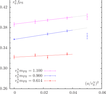
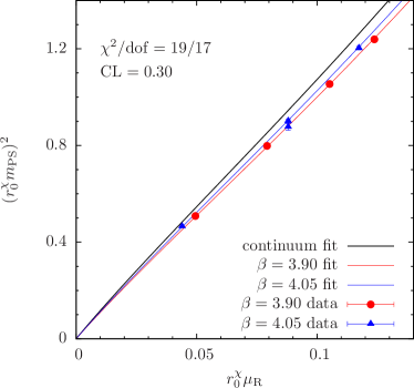
Leading lattice artefacts in our data are expected to be of order $a^{2}$, as discussed previously. This can be checked by extrapolating a physical quantity at fixed physical situation to the continuum limit. We show two such examples in figure 1. In the left panel we show $r^{\chi}_{0}f_{\mathrm{PS}}$ as a function of $(a/r^{\chi}_{0})^{2}$ at fixed value of $r^{\chi}_{0}m_{\mathrm{PS}}$. In order to match the values of $r^{\chi}_{0}m_{\mathrm{PS}}$ at each value of $r^{\chi}_{0}/a$ and to fix the volume to $r_{0}^{\chi}\cdot L=5$ we had to perform short inter- or extra-polations. The straight lines are linear fits in $\left(a/r^{\chi}_{0}\right)^{2}$ to the corresponding data, with the data at the largest value of the lattice spacing not being included in the fit. It is clearly visible that the lattice artefacts appear to scale linearly in $a^{2}$ and that their overall size is small.

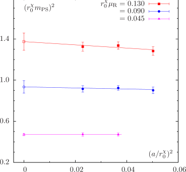
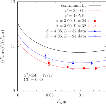
In the right panel we show the scaling of $r^{\chi}_{0}m_{\mathrm{PS}}$ as a function of $(a/r^{\chi}_{0})^{2}$ at fixed values of the renormalised quark mass $r^{\chi}_{0}\mu_{R}$, again at fixed, but finite volume. We conclude that also the charged pseudo scalar mass has only small lattice artefacts. This observation will become particularly important when we shall discuss later the mass difference between charged and neutral pseudo scalar mesons. Note that we do not yet have the value of $Z_{\mathrm{P}}$ for the smallest value of the lattice spacing which is hence left out in fig. 1(b).

The dependence of $m_{\mathrm{PS}}$ and $f_{\mathrm{PS}}$ on the renormalised quark mass and volume can be described by chiral perturbation theory ($\chi$PT) [33, 34, 35]. The residual lattice artefacts of order $a^{2}$ can also be included in the analysis. The corresponding formulae can be found in equation (8) below. We fit these formulae to our data in order to extract the parameters of the $N_{f}=2$ chiral Lagrangian, i.e. the low energy constants and some derived quantities. Moreover, we can use these fits to calibrate our lattices by determining the value of the renormalised quark mass $r^{\chi}_{0}\mu_{R}$ where the ratio $m_{\mathrm{PS}}/f_{\mathrm{PS}}$ assumes its physical value (i.e. $m_{\pi}/f_{\pi}$) and set $f_{\mathrm{PS}}=f_{\pi}=130.7\,\mathrm{MeV}$ there,  as done in ref. [6]. Hence, $f_{\pi}$ is used in this paper to set the scale.

$\Bigl{.}\Bigr{.}$	median	statistical	systematic
$m_{u,d}\ [\mathrm{MeV}]$	$3.54$	$(19)$	$(+16-17)$
$\bar{\ell}_{3}$	$3.50$	$(9)$	$(+9-30)$
$\bar{\ell}_{4}$	$4.66$	$(4)$	$(+4-33)$
$f_{0}\ [\mathrm{MeV}]$	$121.5$	$(0.1)$	$(+1.1-0.1)$
$B_{0}\ [\mathrm{MeV}]$	$2638$	$(149)$	$(\pm 132)$
$r_{0}\ [\mathrm{fm}]$	$0.420$	$(9)$	$(+10-11)$
$|\Sigma|^{1/3}\ [\mathrm{MeV}]$	$270$	$(5)$	$(+3-4)$
$f_{\pi}/f_{0}$	$1.0755$	$(6)$	$(+8-94)$
$r^{\chi}_{0}/a(\beta=3.90)$	$5.32$	$(5)$	$(\pm 0)$
$r^{\chi}_{0}/a(\beta=4.05)$	$6.66$	$(6)$	$(\pm 0)$
$a(\beta=3.90)\ [\mathrm{fm}]$	$0.079$	$(2)$	$(\pm 2)$
$a(\beta=4.05)\ [\mathrm{fm}]$	$0.063$	$(1)$	$(+1-2)$
$Z_{\mathrm{P}}(\beta=3.90)$	$0.434$	$(8)$	$(+4-2)$
$Z_{\mathrm{P}}(\beta=4.05)$	$0.452$	$(9)$	$(+3-9)$

Table 1: Summary of fit results, determined from the weighted distribution as explained in the text. The first error is of statistical origin while the second, the asymmetric one, accounts for the systematic uncertainties. $B_{0}$, $\Sigma$ and $m_{u,d}$ are renormalised in the $\overline{\mathrm{MS}}$ scheme at the renormalisation scale $\mu=2\,\mathrm{GeV}$, as the values of $Z_{\mathrm{P}}$ are in the $\overline{\mathrm{MS}}$ scheme at scale $2\,\mathrm{GeV}$. Note that for the results listed here only data at $\beta=3.9$ and $\beta=4.05$ have been used. The scale is set by $f_{\pi}=130.7\,\mathrm{MeV}$ as done in ref. [6]. For a comparison to other recent lattice results we refer the reader to ref. [2].

The results of these fits can be found in table 1. We give statistical and systematic errors separately, the systematic one being asymmetrical. The results are obtained by performing $\mathcal{O}(80)$ fits, which differ in fit-range, finite size correction formulae and in the order of $\chi$PT. The final result is obtained as the median of the corresponding weighted distribution over all fits. The statistical error is determined using the bootstrap method with 1000 samples. The systematic uncertainty is estimated from the 68% confidence interval of the weighted distribution. For details we refer to the remaining sections of the paper, in particular to appendix A. For a comparison to other lattice results we refer the reader to ref. [2].

The results quoted in table 1 are obtained from the two intermediate values of the lattice spacing only, since at the smallest available lattice spacing $Z_{\mathrm{P}}$ has not yet been computed and the largest value of $a$ is not considered, since there our condition for tuning to maximal twist might not have been fulfilled accurately enough, which may affect in particular the observables $f_{\mathrm{PS}}$ and $m_{\mathrm{PS}}$ (at the smallest quark mass values) considered in this paper. However, including data at the smallest (by fitting $Z_{\mu}=Z_{\mathrm{P}}^{-1}$) and the largest value of the lattice spacing gives results which are compatible within errors with the numbers shown in table 1, as can be seen from a direct comparison in table 7.

3 Ensemble details, $r_{0}$, $a^{2}$ and finite size effects

Before discussing the chiral perturbation theory fits to $m_{\mathrm{PS}}$ and $f_{\mathrm{PS}}$ in section 4 in detail we shall address in this section a number of issues which are needed as preparatory steps. These are the determination of the hadronic scale $r_{0}/a$, the tuning to maximal twist, the size of the $\mathrm{O}(a^{2})$ corrections (including isospin breaking effects) and finite size effects.

3.1 Ensemble Details

In table 2 we summarise the various $N_{f}=2$ ensembles generated by the ETM collaboration. We remark here that all the configurations produced by ETMC are available on the international lattice data grid (ILDG) (see ref. [37] and references therein), and the configurations are made public after publication of this paper. We have simulations at four different values of the inverse gauge coupling $\beta=3.8$, $\beta=3.9$, $\beta=4.05$ and $\beta=4.2$. The corresponding values of the lattice spacing, obtained from chiral fits as detailed later, are $a\approx 0.1\,\mathrm{fm}$, $a\approx 0.079\,\mathrm{fm}$, $a\approx 0.063\,\mathrm{fm}$ and $a\approx 0.051\,\mathrm{fm}$, respectively. For each value of $\beta$ we have several values of the bare twisted mass parameter $a\mu_{q}$, chosen such that the ensembles cover a range of pseudo scalar masses between $280$ and $650\,\mathrm{MeV}$.

The physical box length $L$ of most of the simulations at $\beta=3.9$, $\beta=4.05$ are roughly equal and around $L\approx 2\,\mathrm{fm}$, while the volume at $\beta=3.8$ is slightly larger. At $\beta=4.2$, the lattice size ranges from $L\approx 1.7\,\mathrm{fm}$ to $2.5\,\mathrm{fm}$. For all the values of $\beta$, we demand the condition $m_{\mathrm{PS}}L\gtrsim 3$. Note that we have carried out several simulations at different physical volumes for otherwise fixed parameters in order to study finite size effects (FSE).

The simulation algorithm used to generate these ensembles is a Hybrid Monte Carlo algorithm with multiple time scales and mass preconditioning. It is described in detail in ref. [38] and one implementation described in ref. [39] is freely available. Its performance for the current set-up is discussed in ref. [26]. In table 2 we provide the values of the actual trajectory length $\tau$ used in the simulations. For each value of $\beta$ and $a\mu_{q}$ we have produced around $5000$ equilibrated trajectories in units of $\tau=0.5$. In all cases we allowed for at least $1500$ trajectories for equilibration (again in units of $\tau=0.5$). Some of the ensembles have been produced with a trajectory length $\tau=1$ following the suggestions of ref. [40].

Ensemble	$(L/a)^{3}\times T/a$	$\beta$	$a\mu_{q}$	$\kappa_{\mathrm{crit}}$	$\tau_{\mathrm{int}}(P)$	$\tau_{\mathrm{int}}(am_{\mathrm{PS}})$	$\tau$
$A_{1}$	$24^{3}\times 48$	$3.8$	$0.0060$	$0.164111$	$190(44)$	$8(2)$	$1.0$
$A_{2}$			$0.0080$		$172(80)$	$10(2)$	$1.0$
$A_{3}$			$0.0110$		$130(50)$	$6(1)$	$1.0$
$A_{4}$			$0.0165$		$40(12)$	$6(1)$	$1.0$
$A_{5}$	$20^{3}\times 48$		$0.0060$		$250(100)$	$5(1)$	$1.0$
$B_{1}$	$24^{3}\times 48$	$3.9$	$0.0040$	$0.160856$	$47(15)$	$7(1)$	$0.5$
$B_{2}$			$0.0064$		$23(7)$	$17(4)$	$0.5$
$B_{3}$			$0.0085$		$13(3)$	$10(2)$	$0.5$
$B_{4}$			$0.0100$		$15(4)$	$7(2)$	$0.5$
$B_{5}$			$0.0150$		$30(8)$	$20(6)$	$0.5$
$B_{6}$	$32^{3}\times 64$		$0.0040$		$37(11)$	$2.8(3)$	$0.5$
$B_{7}$			$0.0030$		$51(19)$	$7(1)$	$1.0$
$C_{1}$	$32^{3}\times 64$	$4.05$	$0.0030$	$0.157010$	$18(4)$	$7(1)$	$0.5$
$C_{2}$			$0.0060$		$10(2)$	$9(2)$	$0.5$
$C_{3}$			$0.0080$		$13(3)$	$7(1)$	$0.5$
$C_{4}$			$0.0120$		$5(1)$	$4.8(6)$	$0.5$
$C_{5}$	$24^{3}\times 48$		$0.0060$		$12(2)$	$11(1)$	$1.0$
$C_{6}$	$20^{3}\times 48$		$0.0060$		$10(2)$	$7(1)$	$1.0$
$D_{1}$	$48^{3}\times 96$	$4.2$	$0.0020$	$0.154073$	$13(2)$	$\leq 8$	$1.0$
$D_{2}$	$32^{3}\times 64$		$0.0065$		$6(1)$	$\leq 8$	$1.0$

Table 2: Summary of ensembles generated by ETMC. We give the lattice volume $L^{3}\times T$ and the values of the inverse coupling $\beta$, the twisted mass parameter $a\mu_{q}$, the critical hopping parameter $\kappa_{\mathrm{crit}}$ as determined at $\mu_{q,\mathrm{min}}$ (i.e. the value of $a\mu_{q}$ appearing in the same row as $\kappa_{\mathrm{crit}}$) and the trajectory length $\tau$. The values of the lattice spacing that correspond to the four values of $\beta$ are $a\approx 0.1\,\mathrm{fm}$ ($\beta=3.8$), $a\approx 0.079\,\mathrm{fm}$ ($\beta=3.9$), $a\approx 0.063\,\mathrm{fm}$ ($\beta=4.05$) and $a\approx 0.051\,\mathrm{fm}$ ($\beta=4.2$). In addition we provide values for the integrated autocorrelation time of two typical quantities, the plaquette $P$ and the pseudo scalar mass $am_{\mathrm{PS}}$, in units of $\tau=0.5$. We refer to ref. [9] for details on the determination of the autocorrelation time.

3.2 Hadronic scale parameter $r_{0}$

In order to be able to compare results at different values of the lattice spacing it is convenient to use the hadronic scale $r_{0}$ [32]. It is defined via the force between static quarks and can be measured to high accuracy in lattice QCD simulations. For details on our procedure to determine $r_{0}/a$ we refer to ref. [9]. Note that in this work we use $f_{\pi}$ to set the scale and employ $r_{0}$ only for a continuum limit scaling analysis. In other words $r_{0}^{\chi}$ is used only as an intermediate reference quantity, which is finally eliminated in favour of $f_{\pi}$.

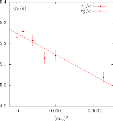
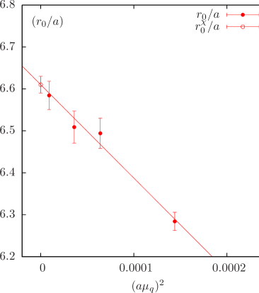
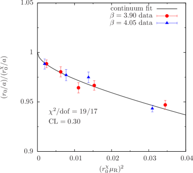
In fig. 2 we show $r_{0}/a$ as a function of $(a\mu_{q})^{2}$ for the examples of $\beta=3.9$ and $\beta=4.05$. The mass dependence appears to be rather weak and a linear fit in $\mu_{q}^{2}$ describes the data well as has been also discussed in refs. [6, 9]. However, also a linear dependence on $a\mu_{q}$ cannot be excluded – due to possible effects of spontaneously broken chiral symmetry in $r_{0}$. This dependence describes in the case of $\beta=3.90$ the data even better than the quadratic ansatz. We shall therefore conservatively include both terms in our final analysis, i.e. the chiral fits discussed in section 4.

For tuning to maximal twist as well as for the continuum-limit scaling analyses presented in this section – in particular in figures 1, 3 and 4 – we shall use the value of $r_{0}^{\chi}/a$ from a linear extrapolation in $(a\mu_{q})^{2}$ to the chiral limit. A linear extrapolation in $(a\mu_{q})^{2}$ yields $r_{0}^{\chi}/a=4.47(6)$ at $\beta=3.8$, $r_{0}^{\chi}/a=5.25(2)$ at $\beta=3.9$, $r_{0}^{\chi}/a=6.61(2)$ at $\beta=4.05$ and $r_{0}^{\chi}/a=8.33(5)$ at $\beta=4.2$. The statistical accuracy for $r^{\chi}_{0}/a$ is about $0.5\%$. It is important to notice that the ratio $[r_{0}^{\chi}/a(\beta=3.9)]/[r_{0}^{\chi}/a(\beta=4.05)]$ is within the errors independent of the extrapolation procedure. This leads us to expect rather little influence of the $r_{0}/a$ extrapolation strategy on physical quantities.

(a)

(b)

Figure 2: $r_{0}/a$ as a function of $(a\mu_{q})^{2}$ for (a) $\beta=3.9$ and (b) $\beta=4.05$. The lines represent a linear extrapolation in $(a\mu_{q})^{2}$ to the chiral limit. Note that we have always used the largest available volume for a given value of $a\mu_{q}$, see table 2.

3.3 Tuning to Maximal Twist

Let us briefly discuss our strategy to tune to maximal twist. It corresponds to tune $am_{0}$ to a critical value $am_{\mathrm{crit}}$ such that the PCAC quark mass defined in eq. (2) vanishes. In particular, we determine the value of $am_{\mathrm{crit}}$ at the lowest available value of $a\mu_{q,\mathrm{min}}\ll a\Lambda_{\mathrm{QCD}}$ at each $\beta$-value. Furthermore, we demand that the ratio $|Z_{\mathrm{A}}am_{\mathrm{PCAC}}/a\mu_{q,\mathrm{min}}|\lesssim 0.1$ and also that its error $\Delta(Z_{\mathrm{A}}am_{\mathrm{PCAC}}/a\mu_{q,\mathrm{min}})\lesssim 0.1$. These criteria and their justification for tuning to maximal twist have been discussed in ref. [9]. An additional condition is that the value of $a\mu_{q,\mathrm{min}}$ corresponds to a fixed physical situation at all values of the lattice spacing. We have chosen to use $m_{\mathrm{PS}}\simeq 300\mathrm{MeV}$ to define the value of $a\mu_{q,\mathrm{min}}$. Considering $\beta=3.9$, $\beta=4.05$ and $\beta=4.2$, it was possible to perform this tuning task with two or three tuning runs for each lattice spacing. Obeying these conditions leads to very small $\mathrm{O}(a^{2})$ effects in the physical observables considered in this paper, with the only exception of the neutral pseudo scalar mass, which will be discussed below.

Figure 3: Renormalised ratio of the PCAC quark mass over the twisted mass against the renormalised twisted mass $\mu_{\mathrm{R}}=\mu_{q}/Z_{\mathrm{P}}$ at the four values of $\beta$. The statistical uncertainties on $Z_{\mathrm{P}}$ and $Z_{\mathrm{A}}$ are not included. The data at $\beta=4.2$ have been included by estimating the renormalisation constants as described in the text. At $\beta=3.8$, the data for the lightest quark mass has not been included for the reasons explained in the text. The band indicates our condition for tuning to maximal twist, which is clearly achieved to a good precision. The arrow indicates the value of $r_{0}^{\chi}\mu_{\mathrm{R}}$ where we tuned the PCAC mass to zero.

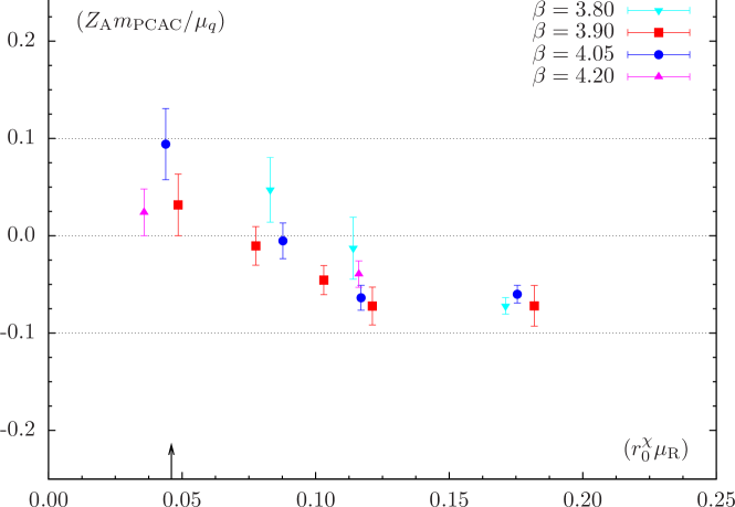
A special case are the simulations at $\beta=3.8$. As can be seen in table 2 at the smallest value of $a\mu_{q}=0.006$ we encounter very large autocorrelation times for the plaquette. Since the autocorrelation time for the PCAC quark mass is of the same order of magnitude as the one of the plaquette, at this value of $a\mu_{q}$ it is questionable whether $am_{\mathrm{PCAC}}$ was reliably determined since the effective statistics is small. Hence, it is unclear whether a tuning to maximal twist fulfilling our conditions has been achieved at $\beta=3.8$. A clarification of this point would have required substantially larger statistics. As a consequence, we will leave out the data at $\beta=3.8$ in our main analysis. The $\beta=3.8$ data will only be discussed in the context of systematic uncertainties.

The measurements of $m_{\mathrm{PCAC}}$ from all the ensembles are collected in Appendix C. In figure 3 we show the properly renormalised ratio of the PCAC quark mass $m_{\mathrm{PCAC}}$ over the twisted mass $\mu_{q}$ (the renormalisation factor of $Z_{\mathrm{P}}$ cancels in this ratio) against the renormalised twisted mass, $\mu_{\mathrm{R}}=\mu_{q}/Z_{\mathrm{P}}$, in units of $r_{0}^{\chi}$, for the four values of $\beta$. The renormalisation factors $Z_{\mathrm{P}}$, taken here at a scale of $2$ GeV, were determined using the RI’-MOM scheme [41, 42]. Note that for $\beta=4.2$ the renormalisation factors are not available yet. However, we have estimated their values by fitting $Z_{\mathrm{P}}$ and by estimating the value of $Z_{A}=0.75$ from the $\beta$-dependence of its known values at smaller $\beta$. Since these renormalisation constants enter as $\mathcal{O}(1)$ multiplicative pre-factors, a small change in their values will not significantly change the data in figure 3. Therefore our main conclusion about the quality of the tuning will be un-altered if the actual numbers for the renormalisation constants should come out slightly differently in the final analysis.

As can be seen from fig. 3 our condition for tuning to maximal twist is satisfied with a good statistical precision. The fact that at the three largest values of $\beta$ the renormalised quark mass computed at the tuning twisted mass parameter $a\mu_{q,\mathrm{min}}$ basically agree (this is illustrated by the arrow in fig. 3) shows in addition that the physical situation has indeed been fixed. At $\beta=3.8$, due to the previously mentioned problem of the long autocorrelation time at the lowest quark mass, we include in fig. 3 only the ensembles for which a reliable estimate of the error on $m_{\mathrm{PCAC}}$ was possible. At all $\beta$-values for values of $a\mu_{q}>a\mu_{q,\mathrm{min}}$ we observe in $am_{\mathrm{PCAC}}$ (small) deviations from zero. This $\mathcal{O}(a)$ cut-off effect will modify only the $\mathcal{O}(a^{2})$ lattice artefacts of physical observables.

3.4 $\mathcal{O}(a^{2})$ effects

In this section, we shall discuss the lattice spacing effects on the decay constant $f_{\mathrm{PS}}$ and the mass $m_{\mathrm{PS}}$ of the (charged) pseudo scalar meson. Starting with $f_{\mathrm{PS}}$, we will use the data at $\beta=3.9$, $\beta=4.05$ and $\beta=4.2$. In order to compare the data at these values of $\beta$, we have fixed three reference values of the pseudo scalar mass to $r^{\chi}_{0}m_{\mathrm{PS}}=0.614$, $r^{\chi}_{0}m_{\mathrm{PS}}=0.90$ and $r^{\chi}_{0}m_{\mathrm{PS}}=1.10$. The corresponding values for $af_{\mathrm{PS}}$ were then obtained by small interpolations, which we have chosen to be linear in $m_{\mathrm{PS}}^{2}$. In addition, we also corrected for the very small differences in the physical volume for the $\beta$ values used such that all data were scaled to the same physical volume $r_{0}^{\chi}\cdot L=5.0$. This has been achieved by applying the relevant formulae from $\chi$PT as detailed below.

As has already been discussed in section 2, in fig. 1(a) (cf. page 1(a)) we show the pseudo scalar decay constant, brought to common reference points $r^{\chi}_{0}m_{\mathrm{PS}}$ and volumes, as a function of $(a/r^{\chi}_{0})^{2}$. In our earlier work, where we had only two values of the lattice spacing [26, 27, 28], we detected only very small lattice spacing artefacts when comparing $\beta=3.9$ and $\beta=4.05$. This observation is confirmed: in fig. 1(a) we now have added, for two values of $a\mu_{q}$, a smaller lattice spacing of $a=0.051\ \mathrm{fm}$ and we can clearly observe that the scaling is as expected linear in $a^{2}$ with only a small slope such that no large cutoff effects are visible. Note that also for the nucleon mass the scaling violations are very small (see refs. [10, 43]).

We also show $r^{\chi}_{0}f_{\mathrm{PS}}$ for $\beta=3.8$ in fig. 1(a) at least for those points where we are able to interpolate to the reference values of $r^{\chi}_{0}m_{\mathrm{PS}}$. Although the linear continuum extrapolation is performed from the results at $\beta=3.9$, $\beta=4.05$ and $\beta=4.2$, as can be seen, the data at $\beta=3.8$ are consistent with this linear behaviour. This indicates that the lattice artefacts are indeed small.

In fig. 1(b) we show similarly the continuum extrapolation of $(r^{\chi}_{0}m_{\mathrm{PS}})^{2}$ for three fixed values of the renormalised quark mass $r^{\chi}_{0}\mu_{\mathrm{R}}=0.045,0.09,0.13$. In this figure we cannot include data at the smallest lattice spacing, due to the missing $Z_{\mathrm{P}}$-factor. Instead we include data from $\beta=3.80$ in the continuum extrapolation to show that the scaling looks very flat. In conclusion also for $(r^{\chi}_{0}m_{\mathrm{PS}})^{2}$ residual scaling violations are small.

3.4.1 Isospin Breaking Effects

A peculiar $\mathrm{O}(a^{2})$ effect in the twisted mass formulation of lattice QCD is the breaking of isospin symmetry at any non-zero value of the lattice spacing. Investigations of these effects deserve therefore special attention. In the quenched approximation the difference $(r_{0}^{\chi})^{2}((m_{\mathrm{PS}}^{\pm})^{2}-(m_{\mathrm{PS}}^{0})^{2})$ between the neutral $m_{\mathrm{PS}}^{0}$ and the charged $m_{\mathrm{PS}}^{\pm}$ pseudo scalar masses, although fully compatible with the expected $\mathrm{O}(a^{2})$ behaviour, turned out to be significant [23].

The determination of $m_{\mathrm{PS}}^{0}$ requires the computation of disconnected diagrams rendering its determination difficult. Nevertheless, following the techniques described in ref. [9], we were able to compute $m_{\mathrm{PS}}^{0}$ (and other neutral quantities) with a reasonable precision. The results for $m_{\mathrm{PS}}^{0}$ and $m_{\mathrm{V}}^{0}$ can be found in table 19 in the appendix.

We show in fig. 4 the mass splitting between the charged and neutral pseudo scalar mesons, i.e.

$$(r_{0}^{\chi})^{2}\ \left[(m_{\mathrm{PS}}^{\pm})^{2}-(m_{\mathrm{PS}}^{0})^{2}\right]$$ (3)

as a function of $(a/r_{0}^{\chi})^{2}$. As can be seen, also for $N_{f}=2$ dynamical quark flavours the isospin breaking effects are large, although smaller than observed in the quenched approximation and of opposite sign, cf. ref. [23], meaning that in the case of dynamical quarks considered here the neutral pseudo scalar meson turns out to be lighter than the charged one. This observation is consistent with the observed first order phase transition [44, 45] and with the corresponding scenario of ref. [46].

One very important observation is that the large cutoff effect in the mass difference between the neutral and charged pseudo scalar masses is dominated by discretisation effects in the neutral pseudo scalar mass. This is demonstrated in fig. 1(b) which shows the charged pseudo scalar mass as a function of $(a/r_{0}^{\chi})^{2}$ for fixed values of $r_{0}^{\chi}\mu_{R}$. As can be seen, the lattice spacing effects are very small, as discussed above.

	$\beta$	$a\mu_{q}$	$R_{O}$
$f_{\mathrm{PS}}$	$3.90$	$0.004$	$0.04(06)$
	$4.05$	$0.003$	$-0.03(06)$
$m_{\mathrm{V}}$	$3.90$	$0.004$	$0.02(07)$
	$4.05$	$0.003$	$-0.05(09)$
$m_{\mathrm{V}}f_{\mathrm{V}}$	$3.90$	$0.004$	$-0.07(18)$
	$4.05$	$0.003$	$-0.31(29)$
$m_{\Delta}$	$3.90$	$0.004$	$0.022(29)$
	$4.05$	$0.003$	$-0.004(45)$

Table 3: Comparison of some selected quantities for which an isospin splitting can occur for twisted mass fermions. $R_{O}$ denotes the relative size of the splitting, see also ref. [24, 25].

Another observation is that, in the unitary sector, so far all other investigated differences between corresponding quantities affected by isospin violations are compatible with zero. In table 3 we have compiled the relative difference $R_{O}=(O-O^{\prime})/O$ for some selected observables and simulation points. Here $O$ ($O^{\prime}$) denotes the charged (neutral) quantity in the case of mesons and $\Delta^{+}$ ($\Delta^{++}$) in the case of baryons. All of them are well compatible with zero. However, some quantities, like the vector meson decay constant $f_{\mathrm{V}}$, are rather noisy and hence the result for this quantity is not really conclusive.

Figure 4: The difference of the squared charged and neutral pseudo scalar masses as a function of $a^{2}$ in the $N_{f}=2$ twisted mass formulation of lattice QCD at two different values of the charged pseudo scalar mass. A significant $\mathrm{O}(a^{2})$ lattice artefact is observed. The circles (triangles) correspond to a value of the charged pion mass of about $330$ ($430$) MeV. The open circle is a larger physical volume. The lines are only to guide the eye and some points are slightly horizontally displaced for better visibility. Note that $r_{0}^{\chi}m_{\mathrm{PS}}^{\pm}$ was not held fixed for this plot, however, due to the large uncertainties on $m_{\mathrm{PS}}^{0}$ the picture should not significantly depend on this approximation.

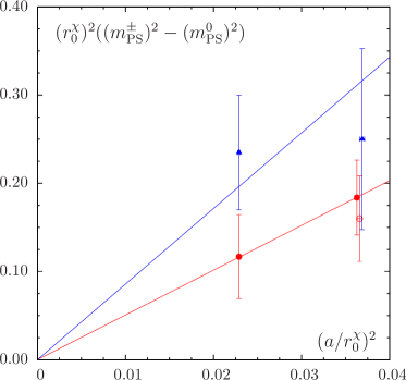
The ETM collaboration has been investigating the question of the large cutoff effects in the neutral pseudo-scalar mass [24, 25, 47] also theoretically. An analysis à la Symanzik of the charged and the neutral pseudo scalar meson masses leads to the formulae

$$\begin{split}(m_{\mathrm{PS}}^{0})^{2}&=m_{\pi}^{2}+a^{2}\zeta_{\pi}+\mathcal{O}(a^{2}m_{\pi}^{2},a^{4})\\ (m_{\mathrm{PS}}^{\pm})^{2}&=m_{\pi}^{2}+\mathcal{O}(a^{2}m_{\pi}^{2},a^{4})\\ \end{split}$$ (4)

which show that the difference $(m_{\mathrm{PS}}^{0})^{2}-(m_{\mathrm{PS}}^{\pm})^{2}$ is given by the term proportional to $\zeta_{\pi}$ (for a discussion in the framework of twisted mass Wilson $\chi$PT see ref. [48, 49]). Here $\zeta_{\pi}\equiv\langle\pi^{0}|\mathcal{L}_{6}|\pi^{0}\rangle$ and $\mathcal{L}_{6}$ is the dimension six term in the Symanzik effective Lagrangian.

The main result of the analysis of ref. [24, 25, 47] is that $\zeta_{\pi}$ is a large number which in the vacuum saturation approximation can be estimated to be proportional to $|\hat{G}_{\pi}|^{2}$, where $\hat{G}_{\pi}=\langle 0|\hat{P}^{3}|\pi^{0}\rangle$. The latter matrix element is numerically large: one finds $|\hat{G}_{\pi}|^{2}/\Lambda_{\mathrm{QCD}}^{4}$ around $20-25$ [24, 25, 47]. This result provides a physical explanation for the large $\mathcal{O}(a^{2})$ effect in the neutral pseudo scalar mass. Moreover, since it can be shown that $\zeta_{\pi}$ appears only in the neutral pseudo scalar mass (and kinematically related quantities), one also finds a possible explanation of why all other splittings determined so far turn out to be small. We remark that in principle also a double insertion of the operator $\mathcal{L}_{5}$ can contribute to the $\mathcal{O}(a^{2})$ lattice artefacts. However, it turns out that these contributions are much smaller than those of $\mathcal{L}_{6}$ discussed here [25].

3.5 Finite Size Effects in $f_{\mathrm{PS}}$ and $m_{\mathrm{PS}}$

In the following, we shall focus on the treatment of finite size effects in $f_{\mathrm{PS}}$ and $m_{\mathrm{PS}}$ with the aim of assessing the applicability of an effective description to be used, in particular, to perform the very small volume corrections required to bring the simulation points to a common finite volume, as needed for the continuum-limit scaling analysis. Later on, in the context of the chiral fits described in section 4, we will apply the finite size corrections formulae to bring our continuum data to infinite volume and to check for systematic effects.

Our lattice data have been obtained with values of $m_{\mathrm{PS}}L\gtrsim 3$. It is generally believed that in such a situation the finite size effects are small and appear only at the per cent level. However, our simulation data are on a level of precision that such effects are certainly detectable and hence finite size effects can in general not be neglected. One possible way to control finite size effects is to use chiral perturbation theory ($\chi$PT) which provides an effective description for the dependence of physical quantities on the box size [50]. A completely independent analytical description of finite size effects (FSE) of particle masses is provided by the so called Lüscher formula developed in ref. [51].

Being interested in $m_{\mathrm{PS}}$ and $f_{\mathrm{PS}}$ – where the applicability of $\chi$PT should be best justified – we then have two effective descriptions of FSE at hand: (i) $\chi$PT to next-to-leading order (NLO) by Gasser and Leutwyler [50], which we shall denote with GL for short, and (ii) the extended asymptotic Lüscher formula of Colangelo, Dürr and Häfeli [52, 53], which conveniently combines the Lüscher formula approach with $\chi$PT and which we will refer to as CDH in the following. Note that in pure $\chi$PT the finite size corrections to $m_{\mathrm{PS}}$ are also known to 2-loop order [54]. However, it turns out that the difference between the CDH formula and 2-loop $\chi$PT is negligible [54].

Below, we compare the numerical data obtained by ETMC to the two different analytical descriptions of the FSE in $m_{\mathrm{PS}}$ and $f_{\mathrm{PS}}$, which is possible since we have precise values for these quantities for a number of ensembles such as $C_{2}$, $C_{5}$ and $C_{6}$ or $B_{1}$ and $B_{6}$ where all parameters but the lattice size are fixed. We remark that for all these ensembles $m_{\mathrm{PS}}L\geq 3$ holds, such that the formulae from refs. [50, 52, 53, 54] should be applicable. This was also checked and discussed in ref. [26].

Starting with the GL ansatz, the finite size corrections for $m_{\mathrm{PS}}$ and $f_{\mathrm{PS}}$ read

$$\begin{split}m_{\mathrm{PS}}(L)&=m_{\mathrm{PS}}\Bigl{[}1+\frac{1}{2}\xi\tilde{g}_{1}(\lambda)\Bigr{]}\equiv m_{\mathrm{PS}}\ K_{m}^{\mathrm{GL}}(L,m_{\mathrm{PS}},f_{0})\,,\\ f_{\mathrm{PS}}(L)&=f_{\mathrm{PS}}\ \Bigl{[}1-2\xi\tilde{g}_{1}(\lambda)\Bigr{]}\ \equiv f_{\mathrm{PS}}\ K_{f}^{\mathrm{GL}}(L,m_{\mathrm{PS}},f_{0})\,,\end{split}$$ (5)

where

$$\xi=m_{\mathrm{PS}}^{2}/(4\pi f_{0})^{2}\,,\qquad\lambda=m_{\mathrm{PS}}L\,,$$ (6)

$\tilde{g}_{1}$ is a known function [50] and the finite size corrections $K_{m,f}^{\mathrm{GL}}$ depend apart from $L$ and $m_{\mathrm{PS}}$ only on the unknown leading order low energy constant $f_{0}$ representing the pseudo scalar decay constant in the chiral limit (note that our normalisation is such that the physical value of the pseudo scalar decay constant is $f_{\pi}=130.7\,\mathrm{MeV}$).

The CDH formulae have a very similar form

$$\begin{split}m_{\mathrm{PS}}(L)&=m_{\mathrm{PS}}\Bigl{[}1-\sum_{n=1}^{\infty}\frac{m(n)}{2\sqrt{n}\lambda}\xi\{I_{m}^{(2)}+\xi I_{m}^{(4)}+\xi^{2}I_{m}^{(6)}+\mathcal{O}(\xi^{3})\}\Bigr{]}\equiv m_{\mathrm{PS}}\ K_{m}^{\mathrm{CDH}}\,,\\ f_{\mathrm{PS}}(L)&=f_{\mathrm{PS}}\Bigl{[}1+\sum_{n=1}^{\infty}\frac{m(n)}{\sqrt{n}\lambda}\xi\{I_{f}^{(2)}+\xi I_{f}^{(4)}+\xi^{2}I_{f}^{(6)}+\mathcal{O}(\xi^{3})\}\Bigr{]}\equiv f_{\mathrm{PS}}\ K_{f}^{\mathrm{CDH}}\,,\\ \end{split}$$ (7)

where the $I_{m,f}^{(i)}$ can be written in terms of basic integrals as discussed in ref. [53], where also $m(n)$ is tabulated. The authors of ref. [53] provide simplified formulae for the $I_{m,f}^{(i)}$, which we shall use in the following. Note that $I_{m}^{(6)}$ is known while $I_{f}^{(6)}$ is not. However, $I_{m}^{(6)}$ is numerically so small that we shall drop it, i.e. set it to zero, in most of what follows. $I_{f}^{(6)}=0$ is always used.

The drawback of the CDH formulae compared to GL is that additional low energy parameters are needed as an input , namely: $\Lambda_{1}$, $\Lambda_{2}$, $\Lambda_{3}$ and $\Lambda_{4}$. However, there are estimates for all those parameters given in ref. [55] and compiled in the form $\bar{\ell}_{i}=\log(\Lambda_{i}^{2}/m_{\pi}^{2})$ in table 4 for convenience, which we shall rely on during the analysis presented in this section. In order to convert the estimates in table 4 into lattice units we conventionally used in this analysis $r^{\chi}_{0}=0.45\,\mathrm{fm}$. Note that the choice of scale here affects only the sub-leading contributions to the finite size corrections and has a negligible effect, as was checked also by direct inspection. We emphasise again that we are at this stage only interested in an effective description of FSE with the goal to understand whether the correction formulae are applicable in the regime of our simulation parameters.

$\bigl{.}\Bigr{.}i$	$\bar{\ell}_{i}$
$1$	$-0.4\pm 0.6$
$2$	$+4.3\pm 0.1$
$3$	$+2.9\pm 2.4$
$4$	$+4.4\pm 0.2$

Table 4: Values for $\bar{\ell}_{i}=\log(\Lambda_{i}^{2}/m_{\pi}^{2})$ from table 2 of ref. [53] used here to analyse FSE.

While the expansion in ref. [55] was performed in terms of the squared pion mass, in ref. [56] the same formulae have been obtained expanding in the quark mass directly. We shall refer to the latter as CDH^m and include it in the following tests.

$\Bigl{.}\Bigr{.}$	$L/a$	$am_{\mathrm{PS}}(L)$	$am_{\mathrm{PS}}^{\mathrm{GL}}(\infty)$	$am_{\mathrm{PS}}^{\mathrm{CDH,6}}(\infty)$	$am_{\mathrm{PS}}^{\mathrm{CDH}}(\infty)$	$am_{\mathrm{PS}}^{\mathrm{CDH^{m}}}(\infty)$
$B_{1}$	$24$	$0.1362(7)$	$0.1354(7)$	$0.1348(7)$	$0.1350(7)$	$0.1346(7)$
$B_{6}$	$32$	$0.1338(2)$	$0.1336(2)$	$0.1335(2)$	$0.1336(2)$	$0.1335(2)$
$C_{6}$	$20$	$0.1520(15)$	$0.1492(15)$	$0.1448(15)$	$0.1464(15)$	$0.1430(15)$
$C_{5}$	$24$	$0.1448(11)$	$0.1436(11)$	$0.1429(11)$	$0.1432(11)$	$0.1418(11)$
$C_{2}$	$32$	$0.1432(06)$	$0.1430(06)$	$0.1429(06)$	$0.1429(06)$	$0.1427(06)$

Table 5: Comparison of different finite size correction formulae of $m_{\mathrm{PS}}$ applied to ensembles where we have different volumes available, while all other parameters stay fixed. $am_{\mathrm{PS}}(L)$ is the measured value, $am_{\mathrm{PS}}^{\mathrm{GL}}(\infty)$ the infinite volume limit value from GL, $am_{\mathrm{PS}}^{\mathrm{CDH,6}}(\infty)$ the infinite volume limit value from CDH, taking $I_{m}^{(6)}$ into account and $am_{\mathrm{PS}}^{\mathrm{CDH}}(\infty)$ and $am_{\mathrm{PS}}^{\mathrm{CDH^{m}}}(\infty)$ the infinite volume limit value from CDH, without $I_{m}^{(6)}$. In the last column the CDH formulae with a re-expansion in the quark mass is used.

$\Bigl{.}\Bigr{.}$	$L/a$	$af_{\mathrm{PS}}(L)$	$af_{\mathrm{PS}}^{\mathrm{GL}}(\infty)$	$af_{\mathrm{PS}}^{\mathrm{CDH}}(\infty)$	$af_{\mathrm{PS}}^{\mathrm{CDH^{m}}}(\infty)$
$B_{1}$	$24$	$0.0646(4)$	$0.0663(4)$	$0.0662(4)$	$0.0663(4)$
$B_{6}$	$32$	$0.0663(2)$	$0.0666(2)$	$0.0665(2)$	$0.0665(2)$
$C_{6}$	$20$	$0.0508(5)$	$0.0546(5)$	$0.0551(5)$	$0.0558(5)$
$C_{5}$	$24$	$0.0558(5)$	$0.0577(5)$	$0.0574(5)$	$0.0578(5)$
$C_{2}$	$32$	$0.0569(2)$	$0.0573(2)$	$0.0572(2)$	$0.0572(2)$

Table 6: same as table 5 but for $f_{\mathrm{PS}}$.

We can now apply the different formulae to correct $m_{\mathrm{PS}}$ and $f_{\mathrm{PS}}$ for finite size effects for ensembles where we have different volumes available. The result can be found in tables 5 and 6. In the tables we show the corrected values at infinite volume from the different ways of treating finite size effects as indicated in the caption. To this end, we take the measured data at a given linear extent $L$ and provide the corresponding correction to infinite volume. For larger volumes these extrapolations agree better and finally converge within the errors. By checking the stability of the values extrapolated to infinite volume from the different analytical formulae we can control the applicability of these corrections for a given lattice size.

All finite size correction formulae provide an appropriate framework to describe the observed finite volume effects. However, for ensembles $B_{1}$ and $C_{6}$, corresponding to the smallest lattice extents at these two $\beta$ values, GL seems to underestimate FSE in $m_{\mathrm{PS}}$, an observation which was also made in refs. [57, 58]. For those cases the resummed Lüscher formula provides a better description. In the chiral fits presented in section 4, however, we observe significantly larger values of $\chi^{2}/\mathrm{d.o.f}$ when GL is used, and hence we use CDH and CDH^m in these fits.

In conclusion, these results make us confident that our simulations have eventually reached a regime of pseudo scalar masses and lattice volumes where $\chi$PT formulae can be used to estimate FSE for $m_{\mathrm{PS}}$ and $f_{\mathrm{PS}}$ when ensembles with $m_{\mathrm{PS}}L\geqslant 3$ are used. In particular, this allows us to control the finite size effects for these mesonic quantities from our simulations. But it is clear that in particular the CDH formula is affected by large uncertainties, mainly stemming from the poorly known low energy constants, which are needed as input. Changing their values in the range suggested in ref. [53], however, changes the estimated finite size effects maximally at the order of about $20\%$ (of the corrections themselves) [9].

Note that in the above discussion we have only used continuum formulae to describe the FSE of our lattice data. However, we believe that this can be justified by the smallness of the lattice artefacts discussed above. In addition, we restate that at this stage we are only interested in an effective but good description of the FSE since our goal was to bring the simulation data from different lattice spacings to a common finite volume as needed to perform the scaling analysis. In all the fits performed later on, the finite size corrections are applied to the continuum results.

4 Combined Fits

The main goal of this section is to confront the data for $f_{\mathrm{PS}}$ and $m_{\mathrm{PS}}$ to $\chi$PT and eventually determine low energy constants (LEC’s) of the chiral effective Lagrangian.

We shall proceed by presenting results from fits including a combined continuum, infinite-volume and chiral extrapolation of $m_{\mathrm{PS}}$ and $f_{\mathrm{PS}}$ for two $\beta$-values, $\beta=3.9$ and $\beta=4.05$. Our analysis will extend the results given in refs. [26, 27] by incorporating data for the renormalisation constant $Z_{\mathrm{P}}$ and the Sommer parameter $r_{0}/a$ in the fit. Details on the computation of $Z_{\mathrm{P}}$ and $r_{0}/a$ can be found in refs. [42, 9]. We shall include the correlation matrix of $f_{\mathrm{PS}}$ and $m_{\mathrm{PS}}$ into the fit (the correlations with $r_{0}/a$ and $Z_{\mathrm{P}}$ are negligible) and also provide a detailed account of systematic uncertainties.

4.1 General Fit Formulae

The formulae we are going to use to describe the chiral and continuum behaviour of $f_{\mathrm{PS}}$, $m_{\mathrm{PS}}$ in infinite volume read:

$$\begin{split}(r_{0}^{\chi}m_{\mathrm{PS}})^{2}&=(r_{0}^{\chi})^{2}\ \chi_{\mu}\Biggl{[}1+\xi\log\left(\frac{\chi_{\mu}}{\Lambda_{3}^{2}}\right)+D_{m_{\mathrm{PS}}}(a/r_{0}^{\chi})^{2}+T_{m}^{\mathrm{NNLO}}\Biggr{]}\ ,\\ r_{0}^{\chi}f_{\mathrm{PS}}&=r_{0}^{\chi}f_{0}\Biggl{[}1-2\xi\log\left(\frac{\chi_{\mu}}{\Lambda_{4}^{2}}\right)+D_{f_{\mathrm{PS}}}(a/r_{0}^{\chi})^{2}+T_{f}^{\mathrm{NNLO}}\Biggr{]}\ ,\\ \end{split}$$ (8)

where $T_{m,f}^{\mathrm{NNLO}}$ denote the continuum NNLO $\chi$PT terms

$$\begin{split}T_{m}^{\mathrm{NNLO}}&=\ \frac{17}{2}\xi^{2}\left[\log\frac{\chi_{\mu}}{\Lambda_{M}^{2}}\right]^{2}+4\xi^{2}k_{M}\ ,\\ T_{f}^{\mathrm{NNLO}}&=\,-5\xi^{2}\left[\log\frac{\chi_{\mu}}{\Lambda_{F}^{2}}\right]^{2}+4\xi^{2}k_{F}\ ,\\ \end{split}$$ (9)

with

$$\begin{split}\log{\frac{\Lambda_{M}^{2}}{\chi_{\mu}}}&=\frac{1}{51}\left(28\log{\frac{\Lambda_{1}^{2}}{\chi_{\mu}}}+32\log{\frac{\Lambda_{2}^{2}}{\chi_{\mu}}}-9\log{\frac{\Lambda_{3}^{2}}{\chi_{\mu}}}+49\right)\ ,\\ \log{\frac{\Lambda_{F}^{2}}{\chi_{\mu}}}&=\frac{1}{30}\left(14\log{\frac{\Lambda_{1}^{2}}{\chi_{\mu}}}+16\log{\frac{\Lambda_{2}^{2}}{\chi_{\mu}}}+6\log{\frac{\Lambda_{3}^{2}}{\chi_{\mu}}}-6\log{\frac{\Lambda_{4}^{2}}{\chi_{\mu}}}+23\right)\ ,\end{split}$$ (10)

and we have defined

$$\xi\equiv\chi_{\mu}/(4\pi f_{0})^{2},\quad\chi_{\mu}\equiv 2B_{0}\mu_{R},\quad\mu_{R}\equiv\mu_{q}/Z_{\mathrm{P}}^{\overline{\mathrm{MS}}}(\mu=2\,\mathrm{GeV})\;.$$ (11)

We use a normalisation such that $f_{0}=\sqrt{2}F_{0}$, i.e. $f_{\pi}=130.7\,\mathrm{MeV}$. For the finite size corrections we shall use the CDH and CDH^m formulae as discussed in sub-section 3.5.

The mass and decay constant of the charged pion have been studied up to NLO [59, 48, 49] in the context of twisted mass chiral perturbation theory (tm$\chi$PT). The regime of quark masses and lattice spacings at which we have performed the simulations is such that $\mu_{R}\gtrsim a\Lambda_{\mathrm{QCD}}^{2}$. In the associated power counting, at maximal twist the NLO tm$\chi$PT expressions for the charged pion mass and decay constant preserve their continuum form. The inclusion of the terms proportional to $D_{m_{\mathrm{PS}},f_{\mathrm{PS}}}$ parametrising the lattice artifacts in eq. (8) represents an effective way of including sub-leading discretisation effects appearing at NNLO. The data shown in fig. 1 (page 1) nicely support the $\mu_{R}$ independence of $D_{f_{\mathrm{PS}},m_{\mathrm{PS}}}$, which we assume in our fit ansatz (8).

$r_{0}^{\chi}$ is the value of the Sommer parameter in the chiral limit which is determined for every $\beta$-value, within the global fit, according to the formula

$$(r_{0}/a)=(r_{0}^{\chi}/a)\ \Bigl{[}1+C_{1}\ r_{0}^{\chi}\mu_{R}+C_{2}\ (r_{0}^{\chi}\mu_{R})^{2}\Bigr{]}$$ (12)

with $\beta$ independent, i.e. continuum parameters $C_{1}$ and $C_{2}$. In addition to the expected $\mu_{R}^{2}$ dependence, we also include the term linear in $\mu_{R}$ in order to account for possible effects of spontaneously broken chiral symmetry. Possible lattice artifacts of $\mathcal{O}(a^{2})$ cannot be distinguished from the lattice artifacts included for $r_{0}^{\chi}m_{\mathrm{PS}}$ and $r_{0}^{\chi}f_{\mathrm{PS}}$ in eq. (8), and are therefore effectively described by the parameters $D_{m_{\mathrm{PS}},f_{\mathrm{PS}}}$, whereas lattice artifacts of order $a^{2}\mu_{R}$ and $a^{2}\mu_{R}^{2}$ appear only at higher order.

In order to work with a massless renormalisation scheme, the values of the pseudo scalar renormalisation constant $Z_{\mathrm{P}}$ are determined in the chiral limit. They were determined using the RI’-MOM scheme at scale $\mu^{\prime}=1/a$ and the values can be found in table 14. For the present fit all renormalisation constants $Z_{\mathrm{P}}$ need to be run from scale $\mu^{\prime}=1/a$ to a common scale, which we have conventionally chosen to be $\mu=2\,\mathrm{GeV}$. This running can be performed perturbatively, but the scale $\mu^{\prime}$ is to be determined. This task can be performed for a given set of fit parameters by setting $f_{\pi}=130.7\,\mathrm{MeV}$ where the ratio $m_{\mathrm{PS}}/f_{\mathrm{PS}}$ assumes its physical value. Hence, we include for $Z_{\mathrm{P}}$

$$Z_{\mathrm{P}}^{\overline{\mathrm{MS}}}(\mu=2\,\mathrm{GeV})=\zeta(\mu,\mu^{\prime})\ Z_{\mathrm{P}}^{\mathrm{RI^{\prime}}}(\mu^{\prime}=1/a)\ /\ R(\mu=2\ \mathrm{GeV}).$$ (13)

into the global fit. $\zeta(\mu,\mu^{\prime})$ describes the running of $Z_{\mathrm{P}}$ from scale $\mu^{\prime}=1/a$ to the scale $\mu=2\,\mathrm{GeV}$ computed in perturbation theory to four loops in $\alpha_{s}$ in ref. [60]. We use the value $\Lambda_{\overline{\mathrm{MS}}}=0.2567\ \mathrm{GeV}$ [61]. The perturbative factor $R(\mu=2\,\mathrm{GeV})=0.8178$ matches the RI’-MOM to the $\overline{\mathrm{MS}}$ scheme and is known to NNNLO. It should be noted that the scale $\mu^{\prime}$ enters only logarithmically into $\zeta$ and the small changes in $\mu^{\prime}$ therefore do make only a very small difference in the running of $Z_{\mathrm{P}}$. However, we include eq. (13) into the global fit in order to correctly account for the statistical uncertainty of $Z_{\mathrm{P}}^{\mathrm{RI^{\prime}}}(\mu^{\prime}=1/a)$.

At NLO, i.e. setting $T_{m,f}^{\mathrm{NNLO}}\equiv 0$, and neglecting finite size corrections for the moment, there are the following free parameters to be fitted to the data for $af_{\mathrm{PS}}$, $am_{\mathrm{PS}}$, $r_{0}/a$ and $Z_{\mathrm{P}}^{\mathrm{RI^{\prime}}}(\mu^{\prime}=1/a)$:

$$r_{0}^{\chi}f_{0},\ r_{0}^{\chi}B_{0},\ r_{0}^{\chi}\Lambda_{3,4},\ C_{1,2},\ \{r_{0}^{\chi}/a\}_{\beta},\ \{Z_{\mathrm{P}}^{\overline{\mathrm{MS}}}(2\ \mathrm{GeV})\}_{\beta},\,\ D_{m_{\mathrm{PS}}},\ D_{f_{\mathrm{PS}}},$$

where we indicate with the notation $\{...\}_{\beta}$ that there is one parameter for each $\beta$-value. When also the NNLO expressions for $m_{\mathrm{PS}}$ and $f_{\mathrm{PS}}$ are included there are four more parameters to be fitted to the data:

$$r_{0}^{\chi}\Lambda_{1,2},\ k_{M},\ k_{F}\ .$$

As already mentioned, finite size effects are corrected for by using the asymptotic formulae from CDH and CDH^m, which is consistently included in the fit. However, both additionally depend on the low energy constants $\Lambda_{1,2}$.

It will turn out that we do not have sufficient data to determine all those parameters from the fit. For this reason we shall add priors for the NNLO low energy constants where needed. A description of the procedure to compute the $\chi^{2}$ can be found in appendix B.

As mentioned above, in our analysis, we find that for a given value of $a\mu_{q}$ and $\beta$ only the data for $am_{\mathrm{PS}}$ and $af_{\mathrm{PS}}$ are correlated and we use a correlated $\chi^{2}$ to account for these. Estimates for the correlation between $af_{\mathrm{PS}}$ and $am_{\mathrm{PS}}$ can be found in the tables 15-18 in appendix C.

4.2 Analysis strategy

By in- and excluding certain data points, we build different data-sets. For a given data-set we perform the following four different fits:

1. Fit A: NLO continuum $\chi$PT, $T_{m,f}^{\mathrm{NNLO}}\equiv 0$, $D_{m_{\mathrm{PS}},f_{\mathrm{PS}}}\equiv 0$, priors for $r_{0}\Lambda_{1,2}$

2. Fit B: NLO continuum $\chi$PT, $T_{m,f}^{\mathrm{NNLO}}\equiv 0$, $D_{m_{\mathrm{PS}},f_{\mathrm{PS}}}$ fitted, priors for $r_{0}\Lambda_{1,2}$

3. Fit C: NNLO continuum $\chi$PT, $D_{m_{\mathrm{PS}},f_{\mathrm{PS}}}\equiv 0$, priors for $r_{0}\Lambda_{1,2}$ and $k_{M,F}$

4. Fit D: NNLO continuum $\chi$PT, $D_{m_{\mathrm{PS}},f_{\mathrm{PS}}}$ fitted, priors for $r_{0}\Lambda_{1,2}$ and $k_{M,F}$

In the above list of different fits, setting $D_{m_{\mathrm{PS}},f_{\mathrm{PS}}}\equiv 0$ corresponds to a constant continuum extrapolation of $f_{\mathrm{PS}}$ and $m_{\mathrm{PS}}$. All these fits are applied to every data-set summarised in table 9, and are repeated with both CDH and CDH^m, respectively. While we include or exclude $m_{\mathrm{PS}}$ and $f_{\mathrm{PS}}$ data corresponding to the data-set, for $r_{0}/a$ we have always used only the largest volume available, since an effective description of finite volume effects is not available for this quantity.

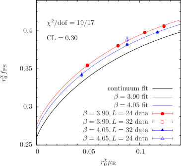
These different fits include the systematic uncertainties of lattice spacing artefacts, finite size effects, higher order contributions in chiral perturbation theory and the extrapolation of $r_{0}/a$ to the chiral limit. Our strategy is to build the distribution of all possible fits using the available data-sets, weighting with the corresponding confidence level. This procedure is analogous to what has been done in ref. [62]. In table 1 we give our best estimates for the fit parameters following this procedure. The best estimates and also quantities derived from those are obtained as the median of the weighted distribution from a total of 76 different fits. All fits are repeated for 1000 bootstrap samples which are used to estimate the statistical errors, while the systematic uncertainties are estimated from the 68% confidence interval of the weighted distribution, as explained in appendix A. As an example we show in figure 5 the result for fit type B on data-set 1, which is also further discussed in the appendix.

(a)

(b)

(c)

(d)

Figure 5: (a) $(r_{0}/a)/(r_{0}^{\chi}/a)$ as a function of $(r^{\chi}_{0}\mu_{\mathrm{R}})^{2}$. (b) $r^{\chi}_{0}f_{\mathrm{PS}}$, (c) $(r^{\chi}_{0}m_{\mathrm{PS}})^{2}$ and (d) $(r^{\chi}_{0}m_{\mathrm{PS}})^{2}/(r^{\chi}_{0}\mu_{\mathrm{R}})$ as a function of $r^{\chi}_{0}\mu_{\mathrm{R}}$. The plots are for fit B on data-set 1. Circles (triangles) represent data points from $\beta=3.90$ ($\beta=4.05$). The value of $\chi^{2}/\mathrm{dof}$ obtained for this fit is $19/17$. Note that in these figures we did not propagate the errors of $r_{0}^{\chi}$ and $Z_{\mathrm{P}}$. When these errors are included the statistical significance of $a^{2}$-dependence of the data in the figures obviously decreases, see table 1.

We exclude fits from the analysis which we consider as being not reasonable, i.e. where the NNLO fit gives a worse description at larger masses than the NLO fit. This is a sign for not having sufficient data for such a fit. In table 1 there are a few quantities which show a strong asymmetry in the estimated systematics. This uncertainty is coming from the fact, that the estimate from NLO and NNLO fits for this quantities differs substantially. However, in the final result the NLO fits have more weight leading to the observed asymmetries.

In order to obtain further confidence in the uncertainties we quote in table 1 we can use the data at $\beta=3.8$ and $\beta=4.20$. In table 7 we compare fits including these data with the results from table 1. It is clearly visible that the overall uncertainty we quote for all the quantities comfortably covers the differences among the three presented fit averages. This fact makes us confident that we indeed have a good estimate of the systematic uncertainties in our results. Note that $Z_{\mathrm{P}}(\beta=4.2)$ is a fit parameter for the fits including data at $\beta=4.2$.

We think that this strategy takes into account all systematic effects that may affect our data and which are accessible to us. This allows us to provide values for the fit parameters and derived quantities with controlled statistical and systematic errors. In particular, since in our fit procedure, finite size corrections are applied in the continuum, effects of the neutral pseudo scalar mass on the finite size effects are absent. The details for our fits can be found in appendix A. Note that the main uncertainty to our results is stemming from our estimates of systematic errors. A systematic effect we are not able to estimate is the missing strange and, possibly, charm quark in the sea.

$\Bigl{.}\Bigr{.}$	$\beta=3.8,3.9,4.05$	$\beta=3.9,4.05$	$\beta=3.9,4.05,4.2$	prior
$m_{u,d}\ [\mathrm{MeV}]$	$3.84(18)$	$3.54(26)$	$3.58(26)$	-
$\bar{\ell}_{3}$	$3.32(21)$	$3.50(31)$	$3.49(9)$	-
$\bar{\ell}_{4}$	$4.69(17)$	$4.66(33)$	$4.63(4)$	-
$\bar{\ell}_{1}$	$-0.41(58)$	$-0.33(62)$	$-0.59(58)$	$-0.4(6)$
$\bar{\ell}_{2}$	$4.31(11)$	$4.32(11)$	$4.32(10)$	$4.3(1)$
$f_{0}\ [\mathrm{MeV}]$	$121.7(3)$	$121.5(1.1)$	$121.58(8)$	-
$B_{0}\ [\mathrm{MeV}]$	$2437(120)$	$2638(200)$	$2619(190)$	-
$r_{0}\ [\mathrm{fm}]$	$0.446(9)$	$0.420(14)$	$0.429(8)$	-
$C_{1}$	$-0.09(18)$	$-0.21(17)$	$-0.37(14)$	-
$C_{2}$	$-1.03(81)$	$-0.52(77)$	$0.09(60)$	-
$\langle r^{2}\rangle_{s}^{\mathrm{NLO}}\ [\mathrm{fm}^{2}]$	$0.710(28)$	$0.715(77)$	$0.710(9)$	-
$|\Sigma|^{1/3}\ [\mathrm{MeV}]$	$262.2(4.0)$	$269.9(6.5)$	$268.4(6.6)$	-
$f_{\pi}/f_{0}$	$1.0742(81)$	$1.0755(94)$	$1.0750(8)$	-
$r^{\chi}_{0}/a(\beta=3.80)$	$4.462(45)$	$-$	$-$	-
$r^{\chi}_{0}/a(\beta=3.90)$	$5.259(48)$	$5.316(49)$	$5.361(39)$	-
$r^{\chi}_{0}/a(\beta=4.05)$	$6.637(57)$	$6.661(62)$	$6.727(48)$	-
$r^{\chi}_{0}/a(\beta=4.20)$	$-$		$8.358(63)$	-
$a(\beta=3.80)\ [\mathrm{fm}]$	$0.0998(19)$	$-$	$-$	-
$a(\beta=3.90)\ [\mathrm{fm}]$	$0.0847(15)$	$0.0790(26)$	$0.0801(14)$	-
$a(\beta=4.05)\ [\mathrm{fm}]$	$0.0672(12)$	$0.0630(20)$	$0.0638(10)$	-
$a(\beta=4.20)\ [\mathrm{fm}]$	$-$	$-$	$0.05142(83)$	-
$Z_{\mathrm{P}}(\beta=3.80)$	$0.431(10)$	$-$	$-$	-
$Z_{\mathrm{P}}(\beta=3.90)$	$0.4390(74)$	$0.4335(84)$	$0.436(9)$	-
$Z_{\mathrm{P}}(\beta=4.05)$	$0.455(10)$	$0.452(13)$	$0.450(11)$	-
$Z_{\mathrm{P}}(\beta=4.20)$	$-$	$-$	$0.466(19)$	$0.45(10)$
$D_{m_{\mathrm{PS}}}$	$0(1)$	$-0.7(1.4)$	$0(2)$	-
$D_{f_{\mathrm{PS}}}$	$0.56(45)$	$1.68(68)$	$1.5(6)$	-

Table 7: We compare fit results of fits including data from $\beta=3.8$ (first data column) and data from $\beta=4.20$ (third data column) with the result where only data from $\beta=3.90$ and $\beta=4.05$ have been used (second data column). Note that in the case of including data from $\beta=4.20$ the value of $Z_{\mathrm{P}}^{\overline{\mathrm{MS}}}$ is determined from the fit. All averages are weighted averages with the confidence levels of the individual fits. The errors are statistical and systematical, added in quadrature. $B_{0}$, $\Sigma$ and $m_{u,d}$ are renormalised in the $\overline{\mathrm{MS}}$ scheme at the renormalisation scale $\mu=2\,\mathrm{GeV}$, as the values of $Z_{\mathrm{P}}$ are in the $\overline{\mathrm{MS}}$ scheme at this scale $\mu$. The scale is set by $f_{\pi}=130.7\,\mathrm{MeV}$ as done in ref. [6].

Eventually it is interesting to investigate the influence of the way $r_{0}/a$ is chirally extrapolated on our final results. In table 1, the systematic effect on $r_{0}^{\chi}/a$ is negligible because of the little variation in the treatment of $r_{0}/a$ between the different fits. Looking at table 7 one might be surprised that the values for $C_{1}$ and $C_{2}$ are both compatible with zero, even if in figure 5(a) a clear mass dependence is visible. The reason for this is that with both parameters the fit is overdetermined and the boostrap samples for $C_{1}$ and $C_{2}$ are strongly anticorrelated ($-0.99$). However, since we are in this analysis not primarily interested in the estimates for $C_{1}$ and $C_{2}$, but more in the correct estimate of systematics for other quantities, we keep both parameters in the fits.

In order to address this systematic effect, we have repeated all the analysis using

$$(r_{0}/a)=(r_{0}^{\chi}/a)\ \Bigl{[}1+C_{2}\ (r_{0}^{\chi}\mu_{R})^{2}\Bigr{]}\ ,$$ (14)

i.e. setting $C_{1}=0$, as compared to eq. (12). In table 8 we compare the results obtained with eq. (14) with the ones presented in table 1. The comparison leads to the conclusion that only the values of $r_{0}^{\chi}/a$ are significantly changed, being also statistically more precise when eq. (14) is used. Thus, the systematic uncertainty stemming from the $r_{0}/a$ extrapolation to the chiral limit is negligible for physical quantities.

$\Bigl{.}\Bigr{.}$	table 1	quadratic
$m_{u,d}\ [\mathrm{MeV}]$	$3.54(26)$	$3.56(29)$
$\bar{\ell}_{3}$	$3.50(31)$	$3.52(48)$
$\bar{\ell}_{4}$	$4.66(33)$	$4.67(25)$
$\bar{\ell}_{1}$	$-0.33(62)$	$-0.50(68)$
$\bar{\ell}_{2}$	$4.32(11)$	$4.33(11)$
$f_{0}\ [\mathrm{MeV}]$	$121.5(1.1)$	$121.48(89)$
$B_{0}\ [\mathrm{MeV}]$	$2638(200)$	$2618(200)$
$r_{0}\ [\mathrm{fm}]$	$0.420(14)$	$0.416(14)$
$C_{1}$	$-0.21(17)$	$-$
$C_{2}$	$-0.52(77)$	$-1.45(14)$
$\langle r^{2}\rangle_{s}^{\mathrm{NLO}}\ [\mathrm{fm}^{2}]$	$0.715(77)$	$0.720(60)$
$|\Sigma|^{1/3}\ [\mathrm{MeV}]$	$269.9(6.5)$	$268.8(6.2)$
$f_{\pi}/f_{0}$	$1.0755(94)$	$1.0759(80)$
$r^{\chi}_{0}/a(\beta=3.90)$	$5.316(49)$	$5.261(14)$
$r^{\chi}_{0}/a(\beta=4.05)$	$6.661(62)$	$6.595(23)$
$a(\beta=3.90)\ [\mathrm{fm}]$	$0.0790(26)$	$0.0790(27)$
$a(\beta=4.05)\ [\mathrm{fm}]$	$0.0630(20)$	$0.0631(21)$
$Z_{\mathrm{P}}(\beta=3.90)$	$0.4335(84)$	$0.4341(90)$
$Z_{\mathrm{P}}(\beta=4.05)$	$0.452(13)$	$0.451(13)$
$D_{m_{\mathrm{PS}}}$	$-0.7(1.4)$	$0.1(1.7)$
$D_{f_{\mathrm{PS}}}$	$1.68(68)$	$2.10(87)$

Table 8: We compare the main results of table 1, where the chiral extrapolation of $r_{0}$ was performed according to eq. (12), with results obtained with the purely quadratic extrapolation of $r_{0}/a$ to the chiral limit in eq. (14). For further details see table 1.

In the tables 1, 7 and 8 we also quote a number of quantities that are derived from the basic fit parameters. The values for the low energy constants $\bar{\ell}_{i}$,

$$\bar{\ell}_{i}=\log\left(\frac{\Lambda_{i}^{2}}{(m_{\pi}^{\pm})^{2}}\right)\;i=1,2,3,4$$ (15)

are determined using the physical value of the charged pion mass $m_{\pi}$, which is the usual convention. The scalar condensate can be determined from the fit parameters $B_{0}$ and $f_{0}$ in the following way:

$$\Sigma=-\frac{B_{0}f_{0}^{2}}{2}$$ (16)

and the scalar radius at next to leading order is given by

$$\langle r^{2}\rangle_{s}^{\mathrm{NLO}}=\frac{12}{(4\pi f_{0})^{2}}(\bar{\ell}_{4}-13/12)\,.$$ (17)

5 Summary and Outlook

In this paper we have demonstrated that Wilson twisted mass fermions, when tuned to maximal twist, show the expected linear scaling in $a^{2}$ with an almost negligible coefficient for both the pseudo scalar decay constant $f_{\mathrm{PS}}$ and mass $m_{\mathrm{PS}}$ (see fig. 1 on page 1). A very similar behaviour is seen for the nucleon mass [10, 43]. It is important to remark that tuning to maximal twist has been achieved in our work by demanding that the renormalised ratio $Z_{\mathrm{A}}m_{\mathrm{PCAC}}/\mu_{q}^{\mathrm{min}}$ of the PCAC mass $m_{\mathrm{PCAC}}$ over the minimal twisted mass $\mu_{q}^{\mathrm{min}}$ employed in our simulations satisfies $|Z_{\mathrm{A}}m_{\mathrm{PCAC}}/\mu_{q}^{\mathrm{min}}|<0.1$. The same condition is used for the corresponding error of this ratio.

The precise data for $f_{\mathrm{PS}}$ and $m_{\mathrm{PS}}$ we have obtained at several values of the lattice spacing, quark masses and volumes allowed for a detailed analysis of systematic effects originating from having to perform a continuum, infinite volume and chiral limit. In particular, in this way it became possible to confront our data to analytical predictions from chiral perturbation theory and to extract a number of low energy constants and derived quantities as listed in table 1, page 1. The main physical results we obtain from this analysis are the light quark mass $m_{u,d}^{\overline{\mathrm{MS}}}(\mu=2\,\mathrm{GeV})=3.54(26)\,\mathrm{MeV}$, the pseudo scalar decay constant in the chiral limit $f_{0}=122(1)\,\mathrm{MeV}$, the scalar condensate $[\Sigma^{\overline{\mathrm{MS}}}(\mu=2\,\mathrm{GeV})]^{1/3}=270(7)\,\mathrm{MeV}$ and $f_{\pi}/f_{0}=1.0755(94)$.

By performing $\mathcal{O}(80)$ different fits, taking into account or leaving out terms describing e.g. lattice artefacts or NNLO chiral perturbation theory and including or excluding data sets, we could achieve a reliable estimate of systematic errors. The final numbers for the fit parameters and their errors were then derived from the median, the bootstrap samples and the 68% confidence level of the (weighted) distribution of fit parameters originating from the different fits. Some quantities such as $\bar{l}_{3}=3.50(31)$, $\bar{l}_{4}=4.66(33)$ or the scalar condensate belong to the most precise determinations available today. For a comparison to other lattice results we refer the reader to ref. [63, 64, 2].

As a particular effect appearing in the twisted mass formulation of lattice QCD, we determined the size of isospin violation in various quantities. In this analysis we found, in accordance with theoretical expectations [24], that only the neutral pseudo scalar mass is significantly affected by the isospin breaking.

We conclude that Wilson twisted mass fermions at maximal twist provide a lattice QCD formulation allowing for precise computations of quantities in the light meson sector of QCD. Clearly, the next step is now to include dynamical strange and charm degrees of freedom in our simulations and work in this direction is in progress [65, 66].

Acknowledgments

The computer time for this project was made available to us by the John von Neumann-Institute for Computing on the JUMP and Jugene systems in Jülich and apeNEXT system in Zeuthen, by UKQCD on the QCDOC machine at Edinburgh, by INFN on the apeNEXT systems in Rome, by BSC on Mare-Nostrum in Barcelona (www.bsc.es), by the Leibniz Computer centre in Munich on the Altix system and by the computer resources made available by CNRS on the BlueGene system at GENCI-IDRIS Grant 2009-052271 and CCIN2P3 in Lyon. We thank these computer centres and their staff for all technical advice and help. On QCDOC we have made use of Chroma [67] and BAGEL [68] software and we thank members of UKQCD for assistance. For the analysis we used among others the R language for statistical computing [69].

This work has been supported in part by the DFG Sonderforschungsbereich/ Transregio SFB/TR9-03 and the EU Integrated Infrastructure Initiative Hadron Physics (I3HP) under contract RII3-CT-2004-506078. We also thank the DEISA Consortium (co-funded by the EU, FP6 project 508830), for support within the DEISA Extreme Computing Initiative (www.deisa.org). G.C.R. and R.F. thank MIUR (Italy) for partial financial support under the contract PRIN04. V.G. and D.P. thank MEC (Spain) for partial financial support under grant FPA2005-00711.

Appendix A Details of fits and discussion of systematics

In this appendix we discuss the details of our data analysis. For a more comprehensive discussion see ref. [36]. For every fit we compute besides the usual $\chi^{2}$ value also the associated confidence levels (CL) (sometimes called goodness of the fit)

$$\mathrm{CL}(q=\chi^{2},n=\mathrm{dof})=1-P(q/2,\ n/2)\,,$$

where $P$ is the incomplete Gamma function which corresponds to the cumulative $\chi^{2}$-distribution function for the given number of degrees of freedom $F_{\chi^{2}}(q,n)$. $F_{\chi^{2}}(q,n)$ itself represents (in the frequentists approach to statistics) the probability of finding a value of $\chi^{2}\leq q$. A confidence level of $\mathrm{CL}(q)=x$ indicates then the fraction of times the computed value of $\chi^{2}$ is larger than $q$, even if the fitted model is correct.

Since we follow a Bayesian approach by including prior knowledge for some parameters into our fits, the interpretation of $\mathrm{CL}$ is more a Bayesian credibility level. Hence, we are not going to determine the most probably correct model on the basis of the values of the CL’s, but we shall rather incorporate all different fits into the final result. The CL’s of each fit are then used as weights, specifying the impact of a given fit on the final result.

In more detail, for obtaining the final results we first sort out all physically un-reasonable fits, as will be described below. Then we generate the CL-weighted distribution of a given fit parameter or of a derived quantity $\theta$ over all the retained fits. The expectation value of $\theta$ is estimated as the median of the weighted distribution. By performing this procedure for every bootstrap sample we determine the statistical error on our estimate for $\theta$. An estimate for the systematic uncertainty is provided by $68.4\%$ confidence interval of the weighted distribution. The estimate for the final error is obtained by adding the statistical and the systematic error in quadrature.

These systematic errors cover effects from lattice artefacts, from different orders in $\chi$PT, finite size effects and fitting range of the quark masses. We present separately the results including data generated at $\beta=3.8$ and $\beta=4.2$, because they are on a different level of accuracy due to insufficient precision in tuning to maximal twist at $\beta=3.8$ and due to the missing estimate of $Z_{\mathrm{P}}^{\mathrm{RI}}$ at $\beta=4.2$. The results for these averages can be found in table 7, in- and excluding $\beta=3.8$ and $\beta=4.2$, compared to the result using only $\beta=3.9$ and $\beta=4.05$ data. The total residual error we quote for our final results covers the difference to the results including $\beta=3.8$ and $\beta=4.2$ data.

As mentioned before, we vary the data-sets in order to probe the influence of the fit range and the finite volume effects on the $\chi$PT fit. The data-sets we use are compiled in table 9. We use both CDH and CDH^m to correct for finite size effects to further check for the influence of those on our results.

The priors for $r_{0}\Lambda_{1,2}$ and $k_{M,F}$ are necessary to obtain stable fits. The priors for $r_{0}\Lambda_{1,2}$ are taken from table 4 and $k_{M,F}=0\pm 10$ is sufficient.

set	$B_{1}$	$B_{2}$	$B_{3}$	$B_{4}$	$B_{5}$	$B_{6}$	$B_{7}$	$C_{1}$	$C_{2}$	$C_{3}$	$C_{4}$	$C_{5}$	$C_{6}$
1	x	x	x	x		x		x	x	x		x
2	x	x	x	x	x	x		x	x	x	x	x
3	x	x	x	x		x	x	x	x	x		x
4	x	x	x	x	x	x	x	x	x	x	x	x
5	x	x	x			x	x	x	x			x
6		x	x	x		x		x	x	x
7		x	x	x	x	x		x	x	x	x
8		x	x	x		x	x	x	x	x
9	x	x	x	x		x		x	x	x			x
10	x	x	x	x	x	x		x	x	x	x		x
11	x	x	x	x		x	x	x	x	x			x
12	x	x	x	x	x	x	x	x	x	x	x		x
13	x	x	x			x	x	x	x				x

set	$A_{2}$	$A_{3}$	$A_{4}$	$B_{1}$	$B_{2}$	$B_{3}$	$B_{4}$	$B_{5}$	$B_{6}$	$B_{7}$	$C_{1}$	$C_{2}$	$C_{3}$	$C_{4}$	$C_{5}$
14	x	x		x	x	x	x		x		x	x	x		x
15	x	x	x	x	x	x	x	x	x		x	x	x	x	x
16	x	x		x	x	x	x		x	x	x	x	x		x
17	x	x	x	x	x	x	x	x	x	x	x	x	x	x	x
18	x			x	x	x			x	x	x	x			x
19	x	x			x	x	x		x		x	x	x
20	x	x	x		x	x	x	x	x		x	x	x	x
21	x	x			x	x	x		x	x	x	x	x

set	$B_{1}$	$B_{2}$	$B_{3}$	$B_{4}$	$B_{5}$	$B_{6}$	$B_{7}$	$C_{1}$	$C_{2}$	$C_{3}$	$C_{4}$	$C_{5}$	$D_{1}$	$D_{2}$
22	x	x	x	x		x		x	x	x		x	x	x
23	x	x	x	x	x	x		x	x	x	x	x	x	x
24	x	x	x	x		x	x	x	x	x		x	x	x
25	x	x	x	x	x	x	x	x	x	x	x	x	x	x
26	x	x	x			x	x	x	x			x	x	x
27		x	x	x		x		x	x	x			x	x
28		x	x	x	x	x		x	x	x	x		x	x
29		x	x	x		x	x	x	x	x			x	x

Table 9: We list the various sets of ensembles used for the fits. We refer to table 2 for the specification of the ensembles used.

NNLO Fits

The NNLO $\chi$PT formulae provide in general a better $\chi^{2}$/d.o.f. than the corresponding NLO formulae. However, it seems that the larger masses with $r_{0}^{\chi}\mu_{\mathrm{R}}\gtrsim 0.14$ are necessary to stabilise these fits. If these masses are left out from the fits then the NNLO fit curves strongly at large values of $r_{0}^{\chi}\mu_{\mathrm{R}}$ and actually undershoots the data at larger masses. This can be seen in figure 6, where we show in the left panel the data for $r_{0}f_{\mathrm{PS}}$ as a function of $r_{0}^{\chi}\mu_{\mathrm{R}}$ and the best fit function for fit C. Note that the data at large values of $r_{0}^{\chi}\mu_{\mathrm{R}}$ are not included in the fit. In the right panel we show the LO, NLO and the complete NNLO function for comparison. Evidently, for larger masses, there is a significant difference between the NLO and NNLO results. It is in particular suspicious that the NNLO fit shows a stronger curvature than the NLO fit and that the NNLO fit deviates more from the data points at large masses – which are not included in the fit. On the contrary one would expect the NNLO formulae to describe the data points at larger masses better than the NLO formulae. On the other hand, when including the heavier masses, the NNLO fit is able to describe these data points. To improve the sensitivity of our lattice data to $\chi$PT at NNLO, additional data points would be needed.

We remark that in ref. [56] the inclusion of NNLO $\chi$PT was found to be necessary in order to obtain an adequate fit to the data on the pion radius. In ref. [56] it was argued that due to the $\rho$-meson dominance one should expect a slower rate of convergence of chiral perturbation theory. However, using the data for $af_{\mathrm{PS}}$ and $am_{\mathrm{PS}}$ alone turns out to be insufficient to obtain the low energy constants at NNLO.

(a)

(b)

Figure 6: We show fit C for data set 1, i.e. including NNLO terms, but excluding lattice artifacts. This fit was not included in the weighted average. In (a) the best fit function for $f_{\mathrm{PS}}$ as a function of the renormalised quark mass. In (b) we plot $f_{\mathrm{PS}}/f_{0}$ in LO, NLO and NNLO for comparison.

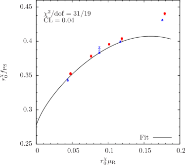
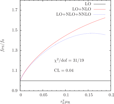
We observe this behaviour for all NNLO fits for data sets without the ensembles at large values of $r_{0}^{\chi}\mu_{\mathrm{R}}\gtrsim 0.14$, therefore, we do not consider these fits as reasonable and exclude them in the weighted average, even if the CL for this fit would justify the inclusion. Note however that including them does not change the final results within the quoted uncertainties.

As already discussed in section 4, one effect of the NNLO fits included in the final analysis is that the estimated systematic uncertainty in e.g. $f_{0}$, $\bar{\ell}_{3}$ and $\bar{\ell}_{4}$ is asymmetric. If we analyse NNLO fits only, we would compared to table 1 rather obtain $f_{0}=122.6(1.1)$, $\bar{\ell}_{3}=3.22(66)$, $\bar{\ell}_{4}=4.33(34)$. This uncertainty is included in our final error estimate of those quantities.

Lattice Artifacts

When performing fit B, which uses only NLO $\chi$PT and includes lattice artifacts, we find that the fitting parameter $D_{m_{\mathrm{PS}}}$ parametrising the lattice artifacts in $m_{\mathrm{PS}}$ is compatible with zero within errors. In $f_{\mathrm{PS}}$ lattice artifacts are more apparent, even if the error on $D_{f_{\mathrm{PS}}}$ is still large.

However, from the fits we clearly observe that the $\chi^{2}$ values are significantly smaller when lattice artifacts are included, and the weighted distribution is hence dominated by the fits of type B and D. As an example for such a fit we show in figure 5 plots for fit B on data-set 1. We show the data together with the fitted curves for $(r_{0}/a)/(r_{0}^{\chi}/a)$ as a function of $(r_{0}^{\chi}\mu_{\mathrm{R}})^{2}$ in (a), for $r_{0}^{\chi}f_{\mathrm{PS}}$ in (b), for $(r_{0}^{\chi}m_{\mathrm{PS}})^{2}$ in (c) and for $(r_{0}^{\chi}m_{\mathrm{PS}})^{2}/(r_{0}^{\chi}\mu_{\mathrm{R}})$ in (d), the last three as a function of $r_{0}^{\chi}\mu_{\mathrm{R}}$. Note that in figures 5(b), 5(c) and 5(d) we did not include the error of $r_{0}^{\chi}$ and $Z_{\mathrm{P}}$ for the data points.

From figure 5 one can observe that the fit works very well, leading to $\chi^{2}/\mathrm{dof}=19/17$. In (a) one can see that the data for $r_{0}/a$ is also fully compatible with a linear dependence on $(r_{0}^{\chi}\mu_{\mathrm{R}})^{2}$ only, as was also discussed earlier and summarised in table 8.

Finite Size Corrections and Effects of Priors

We have used the CDH and CDH^m formulae for the fits and include both into the weighted distribution of all fits. It is still interesting to compare two fits, using CDH^m on the one hand and the parameter free GL formulae on the other hand, while all the rest is identical. We observe that in general the $\chi^{2}$-value using CDH^m is about a factor of 2 smaller than the one using GL. Therefore, we think that having extra parameters (which are included in the fit with priors) is justified.

Another test for uncertainties stemming from FS corrections is to perform fits where only the largest available volume per $\mu_{q}$-value is used. Including these ensembles (which correspond to data-sets 6,7 and 8) tend in general to produce improved values of $\chi^{2}$, while the influence on other fit parameters is again small. Clearly, it would be desirable to have for all ensembles values of $m_{\mathrm{PS}}L>4$, where all the FS correction formulae give very similar results and the uncertainty from finite volumes is hence much reduced. In this investigation we include this significant uncertainty in our final error estimate.

As discussed previously, we have to add priors for $\bar{\ell}_{1,2}$ and $k_{M,F}$ in order to stabilise the fits. It is therefore interesting to discuss the influence of the choice for the priors on the fit results. First of all, the influence of the choice for $k_{M,F}$ and their errors has negligible effect on our fit results.

In case of $\bar{\ell}_{1,2}$ the influence depends on whether or not NNLO terms are included in the chiral expansion. While doubling the error estimates of $\bar{\ell}_{1,2}$ or changing their values within the error range has negligible effects in the case of a NLO chiral fit (fits A and B), many fit results change drastically in the case of NNLO chiral fits (fits C and D): we observe in the latter case that the best fit values e.g. for $\bar{\ell}_{3}$ and $\bar{\ell}_{4}$ differ substantially from the NLO fit result and also from the estimates given in table 4. At the same time the errors become much larger on those quantities, up to 50%.

Moreover, the $\chi^{2}$ minimisation process becomes more difficult, the $\chi^{2}$ functions shows many nearby local minima in parameter space. These facts confirm once more that $f_{\mathrm{PS}}$ and $m_{\mathrm{PS}}$ data are not sensitive to NNLO terms in the chiral expansion.

Chiral Extrapolation of $Z_{\mathrm{P}}^{\mathrm{RI^{\prime}}}$

The chiral extrapolation of $Z_{\mathrm{P}}^{\mathrm{RI^{\prime}}}$ is not performed in the fits, but the chiral value plus error estimates is input to the fit. In order to check whether this might lead the fits into a wrong direction, we have performed fits with doubled uncertainty on the values of $Z_{\mathrm{P}}^{\mathrm{RI^{\prime}}}$. It turns out that this has negligible effect on our results.

Appendix B $\chi^{2}$ Implementation

We are attempting to fit partially correlated data including priors for some of the parameters. With our method we closely follow the approach discussed in ref. [70].

The data for $f_{\mathrm{PS}}$, $m_{\mathrm{PS}}$, $r_{0}/a$ and $Z_{\mathrm{P}}^{\mathrm{RI^{\prime}}}$ at the various values of the lattice spacing and the different volumes is described by the following set of fit parameters

$$r_{0}^{\chi}f_{0},\ r_{0}^{\chi}B_{0},\ r_{0}^{\chi}\Lambda_{1-4},\ k_{M,F},\ C_{1,2},\ \{r_{0}^{\chi}/a\}_{\beta},\ \{Z_{\mathrm{P}}^{\overline{\mathrm{MS}}}(2\ \mathrm{GeV})\}_{\beta},\,\ D_{m_{\mathrm{PS}}},\ D_{f_{\mathrm{PS}}}.$$

With the notation $\{...\}_{\beta}$ we mean that there is one fit parameter for each lattice spacing involved in the fit. Those parameters can be used, employing eqs. (8, 12) and (13), to compute predictions for $am_{\mathrm{PS}}$, $af_{\mathrm{PS}}$, $r_{0}/a$ and $Z_{\mathrm{P}}^{\overline{\mathrm{MS}}}$. We shall denote these predictions by

$$\mathcal{P}_{m_{\mathrm{PS}}},\mathcal{P}_{f_{\mathrm{PS}}},\mathcal{P}_{r_{0}},\mathcal{P}_{Z_{\mathrm{P}}}$$

and they all depend on a sub-list of fit parameters and on the spatial extend $L/a$, as presented in section 4.1.

We adopt the following definition for the $\chi^{2}$-function at fixed value of $\beta$:

$$\begin{split}\chi^{2}(\beta)=&\sum_{a\mu_{q}}\begin{pmatrix}\mathcal{P}_{m_{\mathrm{PS}}}-am_{\mathrm{PS}}\\ \mathcal{P}_{f_{\mathrm{PS}}}-af_{\mathrm{PS}}\\ \end{pmatrix}^{T}C^{-1}\begin{pmatrix}\mathcal{P}_{m_{\mathrm{PS}}}-am_{\mathrm{PS}}\\ \mathcal{P}_{f_{\mathrm{PS}}}-af_{\mathrm{PS}}\\ \end{pmatrix}+\\ &+\sum_{a\mu_{q}}\left(\frac{\mathcal{P}_{r_{0}}-r_{0}/a}{\delta[r_{0}/a]}\right)^{2}+\left(\frac{\mathcal{P}_{Z_{\mathrm{P}}}-Z_{\mathrm{P}}}{\delta[Z_{\mathrm{P}}]}\right)^{2}\ .\end{split}$$ (18)

The matrix $C$ is the properly normalised covariance matrix, see e.g. refs. [71, 72]. The last two terms in eq. (18) are included in order to appropriately include the measurements for $r_{0}/a$ and $Z_{\mathrm{P}}^{\mathrm{RI^{\prime}}}$. Values for the correlation among $m_{\mathrm{PS}}$ and $f_{\mathrm{PS}}$ are given in the tables 15-18. The full $\chi^{2}$ is obtained by summing $\chi^{2}(\beta)$ over all $\beta$-values.

In case we need to add prior knowledge for a fit parameter $\theta$ in order to stabilise the fit we include additional terms of the form

$$\left(\frac{\mathcal{P}_{\theta}-\theta}{\delta[\theta]}\right)^{2}$$ (19)

to the fit, assuming Gaussian error distribution for $\theta$ with standard deviation $\delta[\theta]$. Here the predicted values $\mathcal{P}_{\theta}$ are the fit parameters and the “data” with errors are the priors. The term eq. (19) follows from Bayesian statistics, see ref. [70] and references therein.

In detail the computation of $\chi^{2}$ is performed in the following steps for fixed values of the fit parameters:

1. compute infinite volume and continuum predictions:
   compute the continuum predictions for $m_{\mathrm{PS}}$ and $f_{\mathrm{PS}}$ using the formulae (8) in infinite volume for given values of $r_{0}^{\chi}\mu_{R}$. Determine $r_{0}^{\chi}/a$ for each $\beta$-value according to eq. (12) and use it to estimate the scales $1/a$ from $f_{\pi}$.

2. compute finite volume predictions in the continuum:
   now apply finite size corrections to scale the data to the finite volumes used in the lattice simulations.

3. compute finite $a$ predictions:
   use $r_{0}^{\chi}/a$ to compute the estimates of $am_{\mathrm{PS}}$ and $af_{\mathrm{PS}}$ for finite values of the lattice spacing $a$, depending on the coefficients $D_{m_{\mathrm{PS}},f_{\mathrm{PS}}}$.

4. compute $\chi^{2}$:
   the finite volume and finite $a$ predictions for $m_{\mathrm{PS}}$ and $f_{\mathrm{PS}}$ can now be compared to the data and the $\chi^{2}$ can be computed as detailed above. The $\chi^{2}$ includes also the corresponding terms for the chiral extrapolation of $r_{0}/a$ and for the estimate of $Z_{\mathrm{P}}^{\overline{\mathrm{MS}}}$.

The errors are estimated using the bootstrap method. For $m_{\mathrm{PS}}$ and $f_{\mathrm{PS}}$ we use bootstrap samples as generated from the raw data. For $r_{0}/a$ and $Z_{\mathrm{P}}^{\mathrm{RI^{\prime}}}$ those are generated from a Gaussian distribution with mean and standard-deviation properly chosen. This is justified since we checked that the correlation of $m_{\mathrm{PS}}$ and $f_{\mathrm{PS}}$ to $r_{0}/a$ and $Z_{\mathrm{P}}^{\mathrm{RI^{\prime}}}$ is negligible. This procedure allows to estimate errors on primary quantities, such as fit parameters for instance, as well as on derived quantities, like e.g. the lattice spacing.

Appendix C Data Tables

	$a\mu_{q}$	$am_{\mathrm{PS}}$	$af_{\mathrm{PS}}$	$am_{\mathrm{PCAC}}$	$r_{0}/a$	$L/a$
$A_{1}$	$0.0060$	$0.1852(9)$	$0.0770(8)$	$+0.0019(4)$	$4.321(32)$	$24$
$A_{2}$	$0.0080$	$0.2085(8)$	$0.0835(4)$	$+0.0008(3)$	$4.440(34)$	$24$
$A_{3}$	$0.0110$	$0.2424(5)$	$0.0892(3)$	$-0.0002(5)$	$4.362(21)$	$24$
$A_{4}$	$0.0165$	$0.2957(5)$	$0.0969(2)$	$-0.0017(2)$	$4.264(14)$	$24$
$A_{5}$	$0.0060$	$0.1831(6)$	$0.0784(4)$	$+0.0005(4)$	NA	$20$

Table 10: Data at $\beta=3.8$

	$a\mu_{q}$	$am_{\mathrm{PS}}$	$af_{\mathrm{PS}}$	$am_{\mathrm{PCAC}}$	$r_{0}/a$	$L/a$
$B_{1}$	$0.0040$	$0.1362(7)$	$0.0646(4)$	$+0.00017(17)$	$5.196(28)$	$24$
$B_{2}$	$0.0064$	$0.1694(4)$	$0.0705(4)$	$-0.00009(17)$	$5.216(27)$	$24$
$B_{3}$	$0.0085$	$0.1940(5)$	$0.0742(2)$	$-0.00052(17)$	$5.130(28)$	$24$
$B_{4}$	$0.0100$	$0.2100(5)$	$0.0759(4)$	$-0.00097(26)$	$5.143(25)$	$24$
$B_{5}$	$0.0150$	$0.2586(7)$	$0.0830(3)$	$-0.00145(42)$	$5.039(24)$	$24$
$B_{6}$	$0.0040$	$0.1338(2)$	$0.0663(2)$	$+0.00022(11)$	$5.259(21)$	$32$
$B_{7}$	$0.0030$	$0.1167(4)$	$0.0633(3)$	$+0.00030(14)$	NA	$32$

Table 11: Data at $\beta=3.9$

	$a\mu_{q}$	$am_{\mathrm{PS}}$	$af_{\mathrm{PS}}$	$am_{\mathrm{PCAC}}$	$r_{0}/a$	$L/a$
$C_{1}$	$0.003$	$0.1038(6)$	$0.0500(4)$	$+0.00036(14)$	$6.584(34)$	$32$
$C_{2}$	$0.006$	$0.1432(6)$	$0.0569(2)$	$-0.00004(14)$	$6.509(38)$	$32$
$C_{3}$	$0.008$	$0.1651(5)$	$0.0595(2)$	$-0.00065(13)$	$6.494(36)$	$32$
$C_{4}$	$0.012$	$0.2025(6)$	$0.0644(2)$	$-0.00092(14)$	$6.284(22)$	$32$
$C_{5}$	$0.006$	$0.1448(11)$	$0.0558(5)$	$-0.00027(19)$	NA	$24$
$C_{6}$	$0.006$	$0.1520(15)$	$0.0508(5)$	$+0.00002(20)$	NA	$20$

Table 12: Data at $\beta=4.05$

	$a\mu_{q}$	$am_{\mathrm{PS}}$	$af_{\mathrm{PS}}$	$am_{\mathrm{PCAC}}$	$r_{0}/a$	$L/a$
$D_{1}$	$0.0020$	$0.0740(3)$	$0.0398(2)$	$+0.00006(6)$	$8.295(45)$	$48$
$D_{2}$	$0.0065$	$0.1326(5)$	$0.0465(3)$	$-0.00032(11)$	$8.008(29)$	$32$

Table 13: Data at $\beta=4.20$

$\beta$	$Z_{\mathrm{P}}^{\mathrm{RI^{\prime}}}(\mu^{\prime}=1/a)$
$3.80$	$0.340(10)$
$3.90$	$0.384(08)$
$4.05$	$0.417(11)$

Table 14: Data for $Z_{\mathrm{P}}$ values in the RI’-MOM scheme at scale $\mu^{\prime}=1/a$.

$A_{1}$	$A_{2}$	$A_{3}$	$A_{4}$
$-0.72$	$-0.66$	$-0.03$	$0.06$

Table 15: Correlation among $af_{\mathrm{PS}}$ and $am_{\mathrm{PS}}$ at $\beta=3.8$

$B_{1}$	$B_{2}$	$B_{3}$	$B_{4}$	$B_{5}$	$B_{6}$	$B_{7}$
$-0.53$	$-0.72$	$-0.44$	$0.10$	$0.34$	$-0.62$	$-0.74$

Table 16: Correlation among $af_{\mathrm{PS}}$ and $am_{\mathrm{PS}}$ at $\beta=3.9$

$C_{1}$	$C_{2}$	$C_{3}$	$C_{4}$	$C_{5}$	$C_{6}$
$-0.39$	$-0.44$	$-0.34$	$-0.07$	$-0.41$	$-0.44$

Table 17: Correlation among $af_{\mathrm{PS}}$ and $am_{\mathrm{PS}}$ at $\beta=4.05$

$D_{1}$	$D_{2}$
$-0.44$	$-0.22$

Table 18: Correlation among $af_{\mathrm{PS}}$ and $am_{\mathrm{PS}}$ at $\beta=4.2$

	$am_{\mathrm{PS}}^{\pm}$	$am_{\mathrm{PS}}^{0}$	$am_{\mathrm{V}}^{\pm}$	$am_{\mathrm{V}}^{0}$
$B_{1}$	$0.1362(7)$	$0.109(07)$	$0.404(22)$	$0.391(15)$
$B_{2}$	$0.1694(4)$	$0.134(10)$	$0.422(09)$	$0.434(19)$
$B_{3}$	$0.1940(5)$	$0.169(11)$	$0.428(08)$	$0.424(14)$
$B_{6}$	$0.1338(2)$	$0.110(08)$	$0.416(14)$	$0.409(21)$
$C_{1}$	$0.1038(6)$	$0.090(06)$	$0.335(12)$	$0.352(23)$
$C_{2}$	$0.1432(6)$	$0.123(06)$	$0.347(08)$	$0.344(13)$

Table 19: Comparison of $am_{\mathrm{PS}}^{\pm}$ to $am_{\mathrm{PS}}^{0}$ and $m_{\mathrm{V}}^{\pm}$ to $am_{\mathrm{V}}^{0}$ for the ensembles where the corresponding neutral masses have been computed.

References

- [1] K. Jansen, PoS LATTICE2008, 010 (2008), arXiv:0810.5634 [hep-lat].
- [2] E. E. Scholz, arXiv:0911.2191 [hep-lat].
- [3] ALPHA Collaboration, R. Frezzotti, P. A. Grassi, S. Sint and P. Weisz, JHEP 08, 058 (2001), hep-lat/0101001.
- [4] R. Frezzotti and G. C. Rossi, JHEP 08, 007 (2004), hep-lat/0306014.
- [5] R. Frezzotti and G. C. Rossi, JHEP 10, 070 (2004), hep-lat/0407002.
- [6] ETM Collaboration, P. Boucaud et al., Phys. Lett. B650, 304 (2007), arXiv:hep-lat/0701012.
- [7] ETM Collaboration, B. Blossier et al., JHEP 04, 020 (2008), arXiv:0709.4574 [hep-lat].
- [8] K. Cichy, J. Gonzalez Lopez, K. Jansen, A. Kujawa and A. Shindler, Nucl. Phys. B800, 94 (2008), arXiv:0802.3637 [hep-lat].
- [9] ETM Collaboration, P. Boucaud et al., Comput. Phys. Commun. 179, 695 (2008), arXiv:0803.0224 [hep-lat].
- [10] ETM Collaboration, C. Alexandrou et al., Phys. Rev. D78, 014509 (2008), arXiv:0803.3190 [hep-lat].
- [11] ETM Collaboration, K. Jansen, C. Michael and C. Urbach, Eur. Phys. J. C58, 261 (2008), arXiv:0804.3871 [hep-lat].
- [12] A. Shindler, Phys. Rept. 461, 37 (2008), arXiv:0707.4093 [hep-lat].
- [13] ETM Collaboration, B. Blossier et al., JHEP 07, 043 (2009), arXiv:0904.0954 [hep-lat].
- [14] ETM Collaboration, K. Jansen, C. McNeile, C. Michael and C. Urbach, Phys. Rev. D80, 054510 (2009), arXiv:0906.4720 [hep-lat].
- [15] ETM Collaboration, C. McNeile, C. Michael and C. Urbach, Phys. Lett. B674, 286 (2009), arXiv:0902.3897 [hep-lat].
- [16] B. Blossier et al., arXiv:0909.3187 [hep-lat].
- [17] K. Jansen and A. Shindler, arXiv:0911.1931 [hep-lat].
- [18] L F Collaboration, K. Jansen, A. Shindler, C. Urbach and I. Wetzorke, Phys. Lett. B586, 432 (2004), hep-lat/0312013.
- [19] L F Collaboration, K. Jansen, M. Papinutto, A. Shindler, C. Urbach and I. Wetzorke, Phys. Lett. B619, 184 (2005), hep-lat/0503031.
- [20] L F Collaboration, K. Jansen, M. Papinutto, A. Shindler, C. Urbach and I. Wetzorke, JHEP 09, 071 (2005), hep-lat/0507010.
- [21] A. M. Abdel-Rehim, R. Lewis and R. M. Woloshyn, Phys. Rev. D71, 094505 (2005), hep-lat/0503007.
- [22] R. Frezzotti, G. Martinelli, M. Papinutto and G. C. Rossi, JHEP 04, 038 (2006), hep-lat/0503034.
- [23] L F Collaboration, K. Jansen et al., Phys. Lett. B624, 334 (2005), hep-lat/0507032.
- [24] R. Frezzotti and G. Rossi, PoS LAT2007, 277 (2007), arXiv:0710.2492 [hep-lat].
- [25] P. Dimopoulos, R. Frezzotti, C. Michael, G. C. Rossi and C. Urbach, arXiv:0908.0451 [hep-lat].
- [26] ETM Collaboration, C. Urbach, PoS LAT2007, 022 (2007), arXiv:0710.1517 [hep-lat].
- [27] ETM Collaboration, P. Dimopoulos, R. Frezzotti, G. Herdoiza, C. Urbach and U. Wenger, PoS LAT2007, 102 (2007), arXiv:0710.2498 [hep-lat].
- [28] ETM Collaboration, P. Dimopoulos et al., arXiv:0810.2873 [hep-lat].
- [29] P. Weisz, Nucl. Phys. B212, 1 (1983).
- [30] F. Farchioni et al., Nucl. Phys. Proc. Suppl. 140, 240 (2005), hep-lat/0409098.
- [31] F. Farchioni et al., Eur. Phys. J. C42, 73 (2005), hep-lat/0410031.
- [32] R. Sommer, Nucl. Phys. B411, 839 (1994), hep-lat/9310022.
- [33] S. Weinberg, Physica A96, 327 (1979).
- [34] J. Gasser and H. Leutwyler, Ann. Phys. 158, 142 (1984).
- [35] J. Gasser and H. Leutwyler, Nucl. Phys. B250, 465 (1985).
- [36] Particle Data Group Collaboration, C. Amsler et al., Phys. Lett. B667, 1 (2008).
- [37] T. Yoshie, PoS LATTICE2008, 019 (2008), arXiv:0812.0849 [hep-lat].
- [38] C. Urbach, K. Jansen, A. Shindler and U. Wenger, Comput. Phys. Commun. 174, 87 (2006), hep-lat/0506011.
- [39] K. Jansen and C. Urbach, Comput. Phys. Commun. 180, 2717 (2009), arXiv:0905.3331 [hep-lat].
- [40] H. B. Meyer et al., Comput. Phys. Commun. 176, 91 (2007), arXiv:hep-lat/0606004.
- [41] G. Martinelli, C. Pittori, C. T. Sachrajda, M. Testa and A. Vladikas, Nucl. Phys. B445, 81 (1995), arXiv:hep-lat/9411010.
- [42] P. Dimopoulos et al., PoS LAT2007, 241 (2007), arXiv:0710.0975 [hep-lat].
- [43] C. Alexandrou et al., arXiv:0910.2419 [hep-lat].
- [44] F. Farchioni et al., Eur. Phys. J. C39, 421 (2005), hep-lat/0406039.
- [45] F. Farchioni et al., Phys. Lett. B624, 324 (2005), arXiv:hep-lat/0506025.
- [46] S. R. Sharpe and J. M. S. Wu, Phys. Rev. D70, 094029 (2004), hep-lat/0407025.
- [47] G. Münster, JHEP 09, 035 (2004), hep-lat/0407006.
- [48] L. Scorzato, Eur. Phys. J. C37, 445 (2004), hep-lat/0407023.
- [49] S. R. Sharpe and J. M. S. Wu, Phys. Rev. D71, 074501 (2005), hep-lat/0411021.
- [50] J. Gasser and H. Leutwyler, Phys. Lett. B184, 83 (1987).
- [51] M. Lüscher, Commun. Math. Phys. 104, 177 (1986).
- [52] G. Colangelo and S. Dürr, Eur. Phys. J. C33, 543 (2004), hep-lat/0311023.
- [53] G. Colangelo, S. Dürr and C. Haefeli, Nucl. Phys. B721, 136 (2005), hep-lat/0503014.
- [54] G. Colangelo and C. Haefeli, Nucl. Phys. B744, 14 (2006), arXiv:hep-lat/0602017.
- [55] G. Colangelo, J. Gasser and H. Leutwyler, Nucl. Phys. B603, 125 (2001), arXiv:hep-ph/0103088.
- [56] R. Frezzotti, V. Lubicz and S. Simula, Phys. Rev. D79, 074506 (2009), arXiv:0812.4042 [hep-lat].
- [57] B. Orth, T. Lippert and K. Schilling, Phys. Rev. D72, 014503 (2005), hep-lat/0503016.
- [58] L. Giusti, PoS. LAT2006 (2007), hep-lat/0702014.
- [59] G. Münster and C. Schmidt, Europhys. Lett. 66, 652 (2004), arXiv:hep-lat/0311032.
- [60] K. G. Chetyrkin and A. Retey, Nucl. Phys. B583, 3 (2000), arXiv:hep-ph/9910332.
- [61] ALPHA Collaboration, M. Della Morte et al., JHEP 07, 037 (2008), arXiv:0804.3383 [hep-lat].
- [62] S. Dürr et al., Science 322, 1224 (2008), arXiv:0906.3599 [hep-lat].
- [63] S. Necco, PoS CONFINEMENT8, 024 (2008), arXiv:0901.4257 [hep-lat].
- [64] S. Aoki, arXiv:0910.3806 [hep-lat].
- [65] ETM Collaboration, R. Baron et al., PoS LATTICE2008, 094 (2008), arXiv:0810.3807 [hep-lat].
- [66] ETM Collaboration, R. Baron et al., PoS LATT2009, 104 (2009).
- [67] SciDAC Collaboration, R. G. Edwards and B. Joo, Nucl. Phys. Proc. Suppl. 140, 832 (2005), hep-lat/0409003.
- [68] P. Boyle, http://www.ph.ed.ac.uk/~paboyle/bagel/Bagel.html.
- [69] R Development Core Team, R: A language and environment for statistical computing, R Foundation for Statistical Computing, Vienna, Austria, 2005, ISBN 3-900051-07-0.
- [70] G. P. Lepage et al., Nucl. Phys. Proc. Suppl. 106, 12 (2002), arXiv:hep-lat/0110175.
- [71] C. Michael, Phys. Rev. D49, 2616 (1994), arXiv:hep-lat/9310026.
- [72] C. Michael and A. McKerrell, Phys. Rev. D51, 3745 (1995), arXiv:hep-lat/9412087.