Querying Two Boundary Points for Shortest Paths in a Polygonal Domain

Abstract

We consider a variant of two-point Euclidean shortest path query problem: given a polygonal domain, build a data structure for two-point shortest path query, provided that query points always lie on the boundary of the domain. As a main result, we show that a logarithmic-time query for shortest paths between boundary points can be performed using $\tilde{O}(n^{5})$ preprocessing time and $\tilde{O}(n^{5})$ space where $n$ is the number of corners of the polygonal domain and the $\tilde{O}$-notation suppresses the polylogarithmic factor. This is realized by observing a connection between Davenport-Schinzel sequences and our problem in the parameterized space. We also provide a tradeoff between space and query time; a sublinear time query is possible using $O(n^{3+\epsilon})$ space. Our approach also extends to the case where query points should lie on a given set of line segments.

1 Introduction

A polygonal domains $\mathcal{P}$ with $n$ corners and $h$ holes is a polygonal region of genus $h$ whose boundary consists of $n$ line segments. The holes and the outer boundary of $\mathcal{P}$ are regarded as obstacles. Then, the geodesic distance between any two points $p,q$ in a given polygonal domain $\mathcal{P}$ is defined to be the length of a shortest obstacle-avoiding path between $p$ and $q$.

The Euclidean shortest path problem in a polygonal domain has drawn much attention in the history of computational geometry [15]. In the two-point shortest path query problem, we preprocess $\mathcal{P}$ so that we can determine a shortest path (or its length) quickly for a given pair of query points $p,q\in\mathcal{P}$. While we can compute a shortest path in $O(n\log n)$ time from scratch [13], known structures for logarithmic time query require significantly large storage [6]. Chiang and Mitchell [6] developed several data structures that can answer a two-point query quickly with tradeoffs between storage usage and query time. Most notably, $O(\log n)$ query time can be achieved by using $O(n^{11})$ space and preprocessing time; sublinear query time by $O(n^{5+\epsilon})$ space and preprocessing time. More recently, Guo et al. [10] have shown that a data structure of size $O(n^{2})$ can be constructed in $O(n^{2}\log n)$ time to answer the query in $O(h\log n)$ time, where $h$ is the number of holes. Their results are summarized in Table 1. For more results on shortest paths in a polygonal domain, we refer to survey articles by Mitchell [15, 14].

In this paper, we focus on a variant of the problem, in which possible query points are restricted to a subset of $\mathcal{P}$; the boundary $\partial\mathcal{P}$ of the domain $\mathcal{P}$ or a set of line segments within $\mathcal{P}$. In many applications, possible pairs of source and destination do not span the whole domain $\mathcal{P}$ but a specified subset of $\mathcal{P}$. For example, in an urban planning problem, the obstacles correspond to the residential areas and the free space corresponds to the walking corridors. Then, the query points are restricted to the spots where people depart and arrive, which are on the boundary of obstacles.

Therefore, our goal is to design a data structure using much less resources than structures of Chiang and Mitchell [6] when the query domain is restricted to the boundary of a given polygonal domain $\mathcal{P}$ or to a set of segments in $\mathcal{P}$. To our best knowledge, no prior work seems to investigate this variation. As a main result, in Section 3, we present a data structure of size $O(n^{4}\lambda_{66}(n))$ that can be constructed in $O(n^{4}\lambda_{65}(n)\log n)$ time and can answer a $\partial\mathcal{P}$-restricted two-point shortest path query in $O(\log n)$ time. Here, $\lambda_{m}(n)$ stands for the maximum length of a Davenport-Schinzel sequence of order $m$ on $n$ symbols [19]. It is good to note that $\lambda_{m}(n)=O(n\log^{*}n)$ for any constant $m$ as a convenient intuition, while tighter bounds are known [19, 16]. We also provide a tradeoff between space and query time in Section 4. In particular, we show that one can achieve sublinear query time using $O(n^{3+\epsilon})$ space and preprocessing time. New results in this paper are also summarized in Table 1.

Table 1: Summary of new and known results on exact two-point shortest path queries, where $\epsilon>0$ is arbitrary and $0<\delta\leq 1$ is a parameter. [new] denotes our results.

Query domain	Preprocessing time	Space	Query time	Ref.
$\mathcal{P}$	$O(n^{11})$	$O(n^{11})$	$O(\log n)$	[6]
$\mathcal{P}$	$O(n^{10}\log n)$	$O(n^{10}\log n)$	$O(\log^{2}n)$	[6]
$\mathcal{P}$	$O(n^{5+10\delta+\epsilon})$	$O(n^{5+10\delta+\epsilon})$	$O(n^{1-\delta}\log n)$	[6]
$\mathcal{P}$	$O(n^{5})$	$O(n^{5})$	$O(\log n+h)$	[6]
$\mathcal{P}$	$O(n+h^{5})$	$O(n+h^{5})$	$O(h\log n)$	[6]
$\mathcal{P}$	$O(n^{2}\log n)$	$O(n^{2})$	$O(h\log n)$	[10]
$\partial\mathcal{P}$	$O(n^{4}\lambda_{65}(n)\log n)$	$O(n^{4}\lambda_{66}(n))$	$O(\log n)$	[new]
$\partial\mathcal{P}$	$O(n^{3+\delta}\lambda_{65}(n^{\delta})\log n)$	$O(n^{3+\delta}\lambda_{66}(n^{\delta}))$	$O(n^{1-\delta}\log n)$	[new]
$m$ segments	$O(m^{2}n^{3+\delta}\lambda_{65}(n^{\delta})\log n)$	$O(m^{2}n^{3+\delta}\lambda_{66}(n^{\delta}))$	$O(n^{1-\delta}\log(m+n))$	[new]

Our data structure is a subdivision of two-dimensional domain parameterized in a certain way. The domain is divided into a number of grid cells in which a set of constrained shortest paths between query points have the same structure. Each grid cell is divided according to the projection of the lower envelope of functions stemming from the constrained shortest paths. With careful investigation into this lower envelope, we show the claimed upper bounds.

Also, our approach readily extends to the variant where query points are restricted to lie on a given segment or a given set of segments in $\mathcal{P}$. We discuss this extension in Section 5.

1.1 Related Work

In the case where $\mathcal{P}$ is a simple polygon ($h=0$), the two-point shortest path query can be answered in $O(\log n)$ time after $O(n)$ preprocessing time [9]. More references and results on shortest paths in simple polygons can be found in a survey article by O’Rourke and Suri [17]

Before Chaing and Mitchell [6], fast two-point shortest path queries in polygonal domains were considered as a challenge. Due to this difficulty, many researchers have focused on the approximate two-point shortest path query problem. Chen [5] achieved an $O(n\log n)$-sized structure for $(6+\epsilon)$-approximate shortest path queries in $O(\log n)$ time, and also pointed out that a method of Clarkson [7] can be applied to answer $(1+\epsilon)$-approximate shortest path queries in $O(\log n)$ time using $O(n^{2})$ space and $O(n^{2}\log n)$ preprocessing time. Later, Arikati et al. [4] have improved the above results based on planar spanners.

The problem on polyhedral surfaces also have been considered. Agarwal et al. [1] presented a data structure of size $O(n^{6}m^{1+\delta})$ that answers a two-point shortest path query on a given convex polytope in $O((\sqrt{n}/m^{1/4})\log n)$ time after $O(n^{6}m^{1+\delta})$ preprocessing time for any fixed $1\leq m\leq n^{2}$ and any $\delta>0$. They also considered the problem where the query points are restricted to lie on the edges of the polytope, reducing the bounds by a factor of $n$ from the general case. Recently, Cook IV and Wenk [8] presented an improved method using kinetic Voronoi diagrams.

2 Preliminaries

We are given as input a polygonal domain $\mathcal{P}$ with $h$ holes and $n$ corners. More precisely, $\mathcal{P}$ consists of an outer simple polygon in the plane $\mathbb{R}^{2}$ and a set of $h$ ($\geq 0$) disjoint open simple polygons inside $P$. As a set, $\mathcal{P}$ is the region contained in its outer polygon excluding the holes, also called the free space. The complement of $\mathcal{P}$ in the plane is regarded as obstacles so that any feasible path does not cross the boundary $\partial\mathcal{P}$ and lies inside $\mathcal{P}$. It is well known from earlier works that there exists a shortest (obstacle-avoiding) path between any two points $p,q\in\mathcal{P}$ [14].

Let $V$ be the set of all corners of $\mathcal{P}$. Then any shortest path from $p\in\mathcal{P}$ to $q\in\mathcal{P}$ is a simple polygonal path and can be represented by a sequence of line segments connecting points in $V\cup\{p,q\}$ [14]. The length of a shortest path is the sum of the Euclidean lengths of its segments. The geodesic distance, denoted by $d(p,q)$, is the length of a shortest path between $p$ and $q$. Also, we denote by $|\overline{pq}|$ the Euclidean length of segment $\overline{pq}$.

A two-point shortest path query is given as a pair of points $(p,q)$ with $p,q\in\mathcal{P}$ and asks to find a shortest path between $p$ and $q$. In this paper, we deal with a restriction where the queried points $p$ and $q$ lie on the boundary $\partial\mathcal{P}$.

A shortest path tree $SPT(p)$ for a given source point $p\in\mathcal{P}$ is a spanning tree on the corners $V$ plus the source $p$ such that the unique path to any corner $v\in V$ from the source $p$ in $SPT(p)$ is a shortest path between $p$ and $v$. The combinatorial complexity of $SPT(p)$ for any $p\in\mathcal{P}$ is at most linear in $n$. A shortest path map $SPM(p)$ for the source $p$ is a decomposition of the free space $\mathcal{P}$ into cells in which any point $x$ has a shortest path to $p$ through the same sequence of corners in $V$. Once $SPT(p)$ is obtained, $SPM(p)$ can be computed as an additively weighted Voronoi diagram of $V\cup\{p\}$ with weight assigned by the geodesic distance to $p$ [14]; thus, the combinatorial complexity of $SPM(p)$ is linear. A cell of $SPM(p)$ containing a point $q\in\mathcal{P}$ has the common last corner $v\in V$ along the shortest path from $p$ to $q$; we call such a corner $v$ the root of the cell or of $q$ with respect to $p$. An $O(n\log n)$ time algorithm, using $O(n\log n)$ working space, to construct $SPT(p)$ and $SPM(p)$ is presented by Hershberger and Suri [13].

An SPT-equivalence decomposition $\mathcal{A}^{SPT}$ of $\mathcal{P}$ is the subdivision of $\mathcal{P}$ into cells in which every point has topologically equivalent shortest path tree. An $\mathcal{A}^{SPT}$ can be obtained by overlaying $n$ shortest path maps $SPM(v)$ for every corner $v\in V$ [6]. Hence, the complexity of $\mathcal{A}^{SPT}$ is $O(n^{4})$. Note that $\mathcal{A}^{SPT}\cap\partial\mathcal{P}$ consists of at most $O(n^{2})$ points; they are intersection points between any edge of $SPM(v)$ for any $v\in V$ and the boundary $\partial\mathcal{P}$. We call those intersection points, including the corners $V$, the breakpoints. The breakpoints induce $O(n^{2})$ intervals along $\partial\mathcal{P}$. We shall say that a breakpoint is induced by $SPM(v)$ if it is an intersection of an edge of $SPM(v)$ and $\partial\mathcal{P}$.

Given a set $\Gamma$ of algebraic surfaces and surface patches in $\mathbb{R}^{d}$, the lower envelope $\mathcal{L}(\Gamma)$ of $\Gamma$ is the set of pointwise minima of all given surfaces or patches in the $d$-th coordinate. The minimization diagram $\mathcal{M}(\Gamma)$ of $\Gamma$ is a decomposition of $\mathbb{R}^{d-1}$ into faces, which are maximally connected region over which $\mathcal{L}(\Gamma)$ is attained by the same set of functions. In particular, when $d=3$, the minimization diagram $\mathcal{M}(\Gamma)$ is simply a projection of the lower envelope onto the $xy$-plane. Analogously, we can define the upper envelope and the maximization diagram.

As we intensively exploit known algorithms on algebraic surfaces or surface patches and their lower envelopes, we assume a model of computation in which several primitive operations dealing with a constant number of given surfaces can be performed in constant time: testing if a point lies above, on or below a given surface, computing the intersection of two or three given surfaces, projecting down a given surface, and so on. Such a model of computation has been adopted in many research papers; see [18, 2, 19, 3].

3 Structures for Logarithmic Time Query

In this section, we present a data structure that answers a two-point query restricted on $\partial\mathcal{P}$ in $O(\log n)$ time. To ease discussion, we parameterize the boundary $\partial\mathcal{P}$. Since $\partial\mathcal{P}$ is a union of $h+1$ closed curves, it can be done by parameterizing each curve by arc length and merging them into one. Thus, we have a bijection $p\colon[0,|\partial\mathcal{P}|)\to\partial\mathcal{P}$ that maps a one-dimensional interval into $\partial\mathcal{P}$, where $|\partial\mathcal{P}|$ denotes the total lengths of the $h+1$ closed curves forming $\partial\mathcal{P}$. Conversely, the inverse of $p$ maps each interval along $\partial\mathcal{P}$ to an interval of $[0,|\partial\mathcal{P}|)$.

A shortest path between two points $p,q\in\mathcal{P}$ is either the segment $\overline{pq}$ or a polygonal chain through corners in $V$. Thus, unless $d(p,q)=|\overline{pq}|$, the geodesic distance is taken as the minimum of the following functions $f_{u,v}\colon[0,|\partial\mathcal{P}|)\times[0,|\partial\mathcal{P}|)\to\mathbb{R}$ over all $u,v\in V$, which are defined as follows:

$$f_{u,v}(s,t):=\begin{cases}|\overline{p(s)u}|+d(u,v)+|\overline{vp(t)}|&\text{if $u\in VP(p(s))$ and $v\in VP(p(t))$},\\ \infty&\text{otherwise},\end{cases}$$

where $VP(x)$, for any point $x\in\mathcal{P}$, denotes the visibility profile of $x$, defined as the set of all points $y\in\mathcal{P}$ that are visible from $x$; that is, $\overline{xy}$ lies inside $\mathcal{P}$. The symbol $\infty$ can be replaced by an upper bound of $\max_{s,t}d(p(s),p(t))$; for example, the total length $|\partial\mathcal{P}|$ of the boundary of the polygonal domain $\mathcal{P}$.

Since the case where $p(s)$ is visible from $p(t)$, so the shortest path between them is just the segment $\overline{p(s)p(t)}$, can be checked in $O(\log n)$ time using $O(n^{2}\log n)$ space [6], we assume from now on that $p(s)\notin VP(p(t))$. Hence, our task is to efficiently compute the lower envelope of the $O(n^{2})$ functions $f_{u,v}$ on a 2-dimensional domain $\mathcal{D}:=[0,|\partial\mathcal{P}|)\times[0,|\partial\mathcal{P}|)$.

3.1 Simple lifting to 3-dimension

Using known results on the lower envelope of the algebraic surfaces in $3$-dimension, we can show that a data structure of size $O(n^{6+\epsilon})$ for $O(\log n)$ query can be built in $O(n^{6+\epsilon})$ time as follows.

Fix a pair of intervals $I_{s}$ and $I_{t}$ induced by the breakpoints. Since $I_{s}$ belongs to a cell of an SPT-equivalence decomposition, $VP(p(s))$ is independent of choices over all $s\in I_{s}$. Therefore, the set $V_{s}:=V\cap VP(p(s))$ of corners visible from $p(s)$ is also independent of the choice of $s\in I_{s}$ and further, for a fixed $u\in V_{s}$, there exists a unique $v\in V$ that minimizes $f_{u,v}(s,t)$ for any $(s,t)\in I_{s}\times I_{t}$ over all $v\in V$ [6]. This implies that for each such subdomain $I_{s}\times I_{t}\subset\mathcal{D}$ we extract at most $n$ functions, possibly appearing at the lower envelope. Moreover, in $I_{s}\times I_{t}$, such a function is represented explicitly; for $u\in V_{s}$ and $v\in V_{t}$,

$$f_{u,v}(s,t)=\sqrt{(x(s){-}x_{u})^{2}+(y(s){-}y_{u})^{2}}+d(u,v)+\sqrt{(x(t){-}x_{v})^{2}+(y(t){-}y_{v})^{2}},$$

where $x(s)$ and $y(s)$ are the $x$- and the $y$-coordinates of $p(s)$, and $x_{u}$ and $y_{u}$ are the $x$- and the $y$-coordinates of a point $u\in\mathbb{R}^{2}$. Note that $x(s)$ and $y(s)$ are linear functions in $s$ by our parametrization.

For each $u\in V$, there exists a corner $v\in V_{t}$ that minimizes $f_{u,v^{\prime}}$ in $I_{s}\times I_{t}$ over all $v^{\prime}\in V_{t}$. Therefore, the function $g_{u}:=\min_{v\in V_{t}}f_{u,v}$ on $I_{s}\times I_{t}$ is well-defined. Observe that the graph of $g_{u}$ is an algebraic surface with degree at most $4$ in $3$-dimensional space. Applying any efficient algorithm that computes the lower envelope of algebraic surfaces in $\mathbb{R}^{3}$, we can compute the lower envelope of the functions $g_{u}$ in $O(n^{2+\epsilon})$ time [18]. Repeating this for every such subdomain $I_{s}\times I_{t}$ yields $O(n^{6+\epsilon})$ space and preprocessing time.

Since we would like to provide a point location structure in domain $\mathcal{D}$, we need to find the minimization diagram $\mathcal{M}$ of the computed lower envelope. Fortunately, our domain is $2$-dimensional, so we can easily project it down on $\mathcal{D}$ and build a point location structure with an additional logarithmic factor.

In another way around, one could try to deal with surface patches on the whole domain $\mathcal{D}$. Consider a fixed corner $u\in V$ and its shortest path map $SPM(u)$. The number of breakpoints induced by $SPM(u)$ is at most $O(n)$, including the corners $V$ themselves. This implies at most an $O(n^{2})$ number of combinatorially different paths between any two boundary points $p(s)$ and $p(t)$ via $u$. That is, for a pair of intervals $I_{s}$ and $I_{t}$, we have a unique path via $u$ and its length is represented by a partial function of $(s,t)$ defined on a rectangular subdomain $I_{s}\times I_{t}\subset\mathcal{D}$. Hence, we have $O(n^{2})$ such partial functions for each $u\in V$, and thus $O(n^{3})$ in total. Each of them defines an algebraic surface patch of constant degree on a rectangular subdomain. Consequently, we can apply the same algorithm as above to compute the lower envelope of those patches in $O((n^{3})^{2+\epsilon})=O(n^{6+\epsilon})$ time and space.

3.2 $O(n^{5+\epsilon})$-space structure

Now, we present a way of proper grouping of subdomains to reduce the time/space bound by a factor of $n$. We call a subdomain $I_{s}\times I_{t}\subset\mathcal{D}$, where both $I_{s}$ and $I_{t}$ are intervals induced by breakpoints, a grid cell. Thus, $\mathcal{D}$ consists of $O(n^{4})$ grid cells. We will decompose $\mathcal{D}$ into $O(n^{3})$ blocks of $O(n)$ grid cells.

Consider a pair of boundary edges $S,T\subset\partial\mathcal{P}$ and let $b_{S}$ and $b_{T}$ be the number of breakpoints on $S$ and on $T$, respectively. Let $p(s_{0}),\ldots,p(s_{b_{S}})$ and $p(t_{0}),\ldots,p(t_{b_{T}})$ be the breakpoints on $S$ and on $T$, respectively, in order $s_{0}<s_{1}<\cdots<s_{b_{S}}$ and $t_{0}<t_{1}<\cdots<t_{b_{T}}$. Take $b_{T}$ grid cells with $s\in[s_{0},s_{1})$ and let $\mathcal{C}:=[s_{0},s_{1})\times[t_{0},t_{b_{T}})\subseteq[s_{0},s_{b_{S}})\times[t_{0},t_{b_{T}})$ be their union. We redefine the functions $f_{u,v}$ on domain $\mathcal{C}$. As discussed above, for any $s\in[s_{0},s_{1})$, we have a common subset $V_{s}$ of corners visible from $p(s)$.

For any $u\in V_{s}$, let $g_{u}(s,t):=\min_{v\in V}f_{u,v}(s,t)$ be a function defined on $\mathcal{C}$ and $b_{T}^{u}$ be the number of breakpoints on $T$ induced by $SPM(u)$. The following is our key observation.

Lemma 1

The graph of $g_{u}(s,t)$ on $\mathcal{C}$ consists of at most $b_{T}^{u}+1$ algebraic surface patches with constant maximum degree.

• If $g_{u}(s,t)=f_{u,v}(s,t)$ for any $(s,t)\in\mathcal{C}$ and some $v\in V$, then $p(t)$ lies in a cell of $SPM(u)$ with root $v$; by the definition of $g_{u}$, the involved path goes directly from $p(s)$ to $u$ and follows a shortest path from $u$ to $p(t)$. On the other hand, when we walk along $T$ as $t$ increases from $t_{1}$ to $t_{b_{T}}$, we encounter $b_{T}^{u}$ breakpoints induced by $SPM(u)$; thus, $b_{T}^{u}+1$ cells of $SPM(u)$. Hence, the lemma is shown.

Moreover, the partial function corresponding to each patch of $\gamma_{u}$ is defined on a rectangular subdomain $[s_{0},s_{1})\times[t_{i},t_{j})$ for some $1\leq i<j\leq b_{T}$. This implies that the lower envelope of $g_{u}$ on $\mathcal{C}$ is represented by that of at most $\sum_{u}(b_{T}^{u}+1)=n+b_{T}$ surface patches.

Though this envelope can be computed in $O((n+b_{T})^{2+\epsilon})$ time, we do further decompose $\mathcal{C}$ into $\lceil\frac{b_{T}}{n}\rceil$ blocks of at most $n$ grid cells. This can be simply done by cutting $\mathcal{C}$ at $t=t_{in}$ for each $i=1,\ldots,\lfloor\frac{b_{T}}{n}\rfloor$. For each such block of grid cells, we have at most $2n$ surface patches and thus their lower envelope can be computed in $O(n^{2+\epsilon})$ time. Hence, we obtain the following consequence.

Theorem 1

One can preprocess a given polygonal domain $\mathcal{P}$ in $O(n^{5+\epsilon})$ time into a data structure of size $O(n^{5+\epsilon})$ that answers the two-point shortest path query restricted to the boundary $\partial\mathcal{P}$ in $O(\log n)$-time, where $\epsilon$ is an arbitrarily small positive number.

• Recall that $\sum_{S}b_{S}=\sum_{T}b_{T}=O(n^{2})$. For a pair of boundary edges $S$ and $T$, we can compute the lower envelope of the functions $f_{u,v}$ in $O(b_{S}\lceil\frac{b_{T}}{n}\rceil n^{2+\epsilon})$. Summing this over every pair of boundary edges, we have

  $$\sum_{S,T}O(b_{S}\lceil\frac{b_{T}}{n}\rceil n^{2+\epsilon})=O(n^{4+\epsilon})\cdot\sum_{T}(\frac{b_{T}}{n}+1)=O(n^{5+\epsilon}).$$

  A point location structure on the minimization diagram can be built with additional logarithmic factor, which is subdued by $O(n^{\epsilon})$.

3.3 Further improvement

The algorithms we described so far compute the lower envelope of surface patches in $3$-space in order to obtain the minimization diagram $\mathcal{M}$ of the functions $f_{u,v}$. In this subsection, we introduce a way to compute $\mathcal{M}$ rather directly on $\mathcal{D}$, based on more careful analysis.

Basically, we make use of the same scheme of partitioning the domain $\mathcal{D}$ into blocks of (at most) $n$ grid cells as in Section 3.2. Let $\mathcal{C}$ be such a block defined as $[s_{0},s_{1})\times[t_{0},t_{b_{T}})$ such that $[s_{0},s_{1})$ is an interval induced by the breakpoints and $[t_{0},t_{b_{T}})$ is a union of $b_{T}\leq n$ consecutive intervals in which we have $b_{T}-1$ breakpoints $t_{1},\dots,t_{b_{T}-1}$.

By Lemma 1, the functions $g_{u}=\min_{v\in V}f_{u,v}$ restricted to $\mathcal{C}$ can be split into at most $2n$ partial functions $h_{i}$ with $1\leq i\leq 2n$ defined on a subdomain $\mathcal{C}_{i}\subseteq\mathcal{C}$. Each $h_{i}(s,t)$ is represented explicitly as $h_{i}(s,t)=|p(s)u_{i}|+d(u_{i},v_{i})+|v_{i}p(t)|$ in $\mathcal{C}_{i}$, so that we have $h_{i}(s,t)=f_{u_{i},v_{i}}(s,t)$ for any $(s,t)\in\mathcal{C}_{i}$ and some $u_{i},v_{i}\in V$. Note that it may happen that $u_{i}=u_{j}$ or $v_{i}=v_{j}$ for some $i$ and $j$; in particular, if $u_{i}=u_{j}$, we have $\mathcal{C}_{i}\cap\mathcal{C}_{j}=\emptyset$. Also, as discussed in Section 3.2, $\mathcal{C}_{i}$ is represented as $[s_{0},s_{1})\times[t_{k},t_{k^{\prime}})$ for some $0\leq k<k^{\prime}\leq b_{T}$.

In this section, we take the partial functions $h_{i}$ into account, and thus the goal is to compute the minimization diagram $\mathcal{M}$ of surface patches defined by the $h_{i}$. We start with an ordering on the set $V_{s}$ of corners visible from $p(s)$ for any $s\in[s_{0},s_{1})$ based on the following observation.

Lemma 2

The angular order of corners in $V_{s}$ seen at $s$ is constant if $s$ varies within $[s_{0},s_{1})$.

• If this is not true, we have such an $s^{\prime}\in[s_{0},s_{1})$ that $p(s^{\prime})$ and two corners $v,v^{\prime}$ in $V_{s}$ are collinear. Since corners lie on the boundary of an obstacle, one of $v$ and $v^{\prime}$ is not visible from $p(s)$ locally near $s^{\prime}$; that is, $p(s^{\prime})$ is a breakpoint, a contradiction.

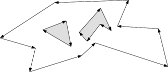
Figure 1: As $s$ increases, $p(s)$ moves in direction where the obstacle is to the right.

Without loss of generality, we assume that as $s$ increases, $p(s)$ moves along $\partial\mathcal{P}$ in direction that the obstacle lies to the right; that is, $p(s)$ moves clockwise around each hole and counter-clockwise around the outer boundary of $\mathcal{P}$. (See Figure 1.) By Lemma 2, we order the corners in $V_{s}$ in counter-clockwise order at $p(s)$ for any $s\in[s_{0},s_{1})$; let $\prec$ be a total order on $V_{s}$ such that $u\prec u^{\prime}$ if and only if $\angle p(s_{0})p(s)u<\angle p(s_{0})p(s)u^{\prime}$.

From now on, we investigate the set

$$B(i,j):=\{(s,t)\in\mathcal{C}_{i}\cap\mathcal{C}_{j}\mid h_{i}(s,t)=h_{j}(s,t)\},$$

which is a projection of the intersection of two surface patches defined by $h_{i}$ and $h_{j}$. One can easily check that $B(i,j)$ is a subset of an algebraic curve of degree at most $8$.

Lemma 3

The set $B(i,j)$ is $t$-monotone. That is, for fixed $t$, there is at most one $s\in[s_{0},s_{1})$ such that $(s,t)\in B(i,j)$.

If $(s,t)\in B(i,j)$, we have equation $h_{i}(s,t)=h_{j}(s,t)$. From the equation, we get $|p(s)u_{i}|-|p(s)u_{j}|=|v_{j}p(t)|+d(u_{j},v_{j})-|v_{i}p(t)|-d(u_{i},v_{i})$. If we fix $t$ as constant, $|p(s)u_{i}|-|p(s)u_{j}|$ remains a constant even if $s$ varies within $[s_{0},s_{1})$. Thus, $p(s)$ is an intersection point with line segment $\overline{p(s_{0})p(s_{1})}$ and a branch $H$ of a hyperbola whose foci are $u_{i}$ and $u_{j}$. If $\overline{p(s_{0})p(s_{1})}\cap H$ consists of two points, then the line $\ell$ through $u_{i}$ and $u_{j}$ must cross $\overline{p(s_{0})p(s_{1})}$ at a point $z$; $\ell$ is the transverse axis of $H$ and both $u_{i}$ and $u_{j}$ lie in one side of the line supporting $\overline{p(s_{0})p(s_{1})}$. Such a crossing point $z$ is a breakpoint by definition but we do not have any breakpoint within $\overline{p(s_{0})p(s_{1})}$ since $[s_{0},s_{1})$ is an interval induced by the breakpoints, a contradiction.

Lemma 4

The set $B(i,j)$ is either an empty set or an open curve whose endpoints lie on the boundary of $\mathcal{C}_{i}\cap\mathcal{C}_{j}$. Moreover, $B(i,j)$ is either a linear segment parallel to the $t$-axis or $s$-monotone.

• Let $I_{s}$ and $I_{t}$ be intervals such that $\mathcal{C}_{i}\cap\mathcal{C}_{j}=I_{s}\times I_{t}$. Note that $I_{s}=[s_{0},s_{1})$ and $I_{t}=[t_{k},t_{k^{\prime}})$ for some $0\leq k<k^{\prime}\leq b_{T}$.

  First, note that if $u_{i}=u_{j}$, $\mathcal{C}_{i}\cap\mathcal{C}_{j}=\emptyset$ and thus $B(i,j)=\emptyset$, so the lemma is true. Thus, we assume that $u_{i}\neq u_{j}$. Regarding $v_{i}$ and $v_{j}$, there are two cases: $v_{i}=v_{j}$ or $v_{i}\neq v_{j}$. In the former case, we get $|p(s)u_{i}|-|p(s)u_{j}|=d(u_{j},v_{j})-d(u_{i},v_{i})$ from equation $h_{i}(s,t)=h_{j}(s,t)$. Observe that variable $t$ is readily eliminated from the equation, and thus if there exists $(s^{\prime},t^{\prime})\in\mathcal{C}_{i}\cap\mathcal{C}_{j}$ with $(s^{\prime},t^{\prime})\in B(i,j)$, we have $(s^{\prime},t)\in B(i,j)$ for every other $t\in I_{t}$. Hence, by Lemma 3, $B(i,j)$ is empty or a straight line segment in $\mathcal{C}_{i}\cap\mathcal{C}_{j}$ which is parallel to $t$-axis, and thus the lemma is shown.

  Now, we consider the latter case where $v_{i}\neq v_{j}$. Without loss of generality, we assume that $u_{i}\prec u_{j}$. Recall that if $u_{i}\prec u_{j}$, then $\angle p(s_{0})p(s)u_{i}<\angle p(s_{0})p(s)u_{j}$ for any $s$ in the interior of $I_{s}$. We denote $\theta_{i}(s):=\angle p(s_{0})p(s)u_{i}$ and $\theta_{j}(s):=\angle p(s_{0})p(s)u_{j}$. On the other hand, we also have a similar relation for $v_{i}$ and $v_{j}$. Let $\phi_{i}(t):=\angle p(t_{0})p(t)v_{i}$ and $\phi_{j}(t):=\angle p(t_{0})p(t)v_{j}$. Observe that $\phi_{i}(t)$ and $\phi_{j}(t)$ are continuous functions of $t$, and if $\phi_{i}(t^{\prime})=\phi_{j}(t^{\prime})$ at $t=t^{\prime}$, then $p(t^{\prime})$ is a breakpoint induced by $SPM(u_{i})$ or $SPM(u_{j})$. Since $I_{t}$ contains no such breakpoint induced by $SPM(u_{i})$ or $SPM(u_{j})$ in its interior, either $\phi_{i}(t)<\phi_{j}(t)$ or $\phi_{i}(t)>\phi_{j}(t)$ for all $t$ in the interior of $I_{t}$; that is, the sign of $\phi_{j}(t)-\phi_{i}(t)$ is constant.

Since for any $s,s^{\prime}\in I_{s}$ with $s^{\prime}>s$ we have $|p(s^{\prime})p(s)|=s^{\prime}-s$ by our parametrization, we can represent $|p(s)u_{i}|=\sqrt{(s+a_{i})^{2}+b_{i}^{2}}$ and $|v_{i}p(t)|=\sqrt{(t+c_{i})^{2}+d_{i}^{2}}$, where $a_{i}$, $b_{i}$, $c_{i}$ and $d_{i}$ are constants depending on $u_{i}$, $v_{i}$, and parametrization $p$. More specifically, $s+a_{i}$ denotes a signed distance between $p(s)$ and the perpendicular foot of $u_{i}$ onto the line supporting $p(I_{s})$, and $b_{i}$ is the distance between $u_{i}$ and the line supporting $p(I_{s})$. See Figure 2. Thus, $h_{i}(s,t)$ can represented as $h_{i}(s,t)=\sqrt{(s+a_{i})^{2}+b_{i}^{2}}+\sqrt{(t+c_{i})^{2}+d_{i}^{2}}+d(u_{i},v_{i})$.

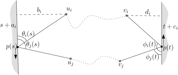
Figure 2: Illustration to the proof of Lemma 4

Now, we differentiate the both sides of equation $h_{i}(s,t)=h_{j}(s,t)$ by $t$ to obtain the derivative $\frac{ds}{dt}$:

$$\frac{s+a_{i}}{\sqrt{(s+a_{i})^{2}+b_{i}^{2}}}\frac{ds}{dt}+\frac{t+c_{i}}{\sqrt{(t+c_{i})^{2}+d_{i}^{2}}}=\frac{s+a_{j}}{\sqrt{(s+a_{j})^{2}+b_{j}^{2}}}\frac{ds}{dt}+\frac{t+c_{j}}{\sqrt{(t+c_{j})^{2}+d_{j}^{2}}}.$$

Rearranging this, we obtain

$$\frac{ds}{dt}=\frac{\displaystyle-\frac{t+c_{i}}{\sqrt{(t+c_{i})^{2}+d_{i}^{2}}}+\frac{t+c_{j}}{\sqrt{(t+c_{j})^{2}+d_{j}^{2}}}}{\displaystyle\frac{s+a_{i}}{\sqrt{(s+a_{i})^{2}+b_{i}^{2}}}-\frac{s+a_{j}}{\sqrt{(s+a_{j})^{2}+b_{j}^{2}}}}=\frac{-\cos(\phi_{i}(t))+\cos(\phi_{j}(t))}{\cos(\theta_{i}(s))-\cos(\theta_{j}(s))}.$$

Since $0<\theta_{i}(s)<\theta_{j}(s)<\pi$, we have $\cos(\theta_{i}(s))-\cos(\theta_{j}(s))>0$. Also, as discussed above, $\phi_{j}(t)-\phi_{i}(t)$ has a constant sign when $t$ varies within the interior of $I_{t}$. Thus, $\cos(\phi_{j}(t))-\cos(\phi_{i}(t))$ has a constant sign, and $\frac{ds}{dt}$ also has a constant sign at any $(s,t)\in B(i,j)$. Furthermore, $\frac{ds}{dt}$ is continuous and has no singularity in the interior of $\mathcal{C}_{i}\cap\mathcal{C}_{j}$. This, together with Lemma 3, proves the lemma.

Now, we know that $B(i,j)$ can be seen as the graph of a partial function $\{s=\gamma(t)\}$. Also, Lemma 4 implies that $B(i,j)$ bisects $\mathcal{C}_{i}\cap\mathcal{C}_{j}$ into two connected regions $R(i,j)$ and $R(j,i)$, where $R(i,j):=\{(s,t)\in\mathcal{C}_{i}\cap\mathcal{C}_{j}\mid h_{i}(s,t)<h_{j}(s,t)\}$ and $R(j,i):=\{(s,t)\in\mathcal{C}_{i}\cap\mathcal{C}_{j}\mid h_{i}(s,t)>h_{j}(s,t)\}$. Let $\mathcal{M}(i)$ be the set of points $(s,t)$ where the minimum of $h_{j}(s,t)$ over all $j$ is attained by $h_{i}(s,t)$. We then have $\mathcal{M}(i)=\mathcal{C}_{i}\setminus\bigcup_{j}R(j,i)$ for each $i$.

For easy explanation, from now on, we regard the $s$-axis as the vertical axis in $\mathcal{D}$ so that we can say a point lies above or below a curve in this sense.

The idea of computing $\mathcal{M}(i)$ is to use the lower and the upper envelopes of the bisecting curves $B(i,j)$. In order to do so, we extend $B(i,j)$ to cover the whole $t$-interval $I_{t}=[t_{k},t_{k^{\prime}})$ in $\mathcal{C}_{i}\cap\mathcal{C}_{j}$ by following operation: For each endpoint of $B(i,j)$, if it does not lie on the vertical line $\{t=t_{k}\}$ or $\{t=t_{k^{\prime}}\}$, attach a horizontal segment to reach the vertical line as shown in Figure 3(a). We denote the resulting curve by $\beta(i,j)$; if $B(i,j)=\emptyset$, define $\beta(i,j)$ as the horizontal segment connecting two points $(s_{0},t_{k})$ and $(s_{0},t_{k^{\prime}})$ in $\mathcal{C}_{i}\cap\mathcal{C}_{j}$. Observe now that $\beta(i,j)$ bisects $\mathcal{C}_{i}\cap\mathcal{C}_{j}$ into regions $R(i,j)$ and $R(j,i)$, which lie above and below $\beta(i,j)$, respectively.

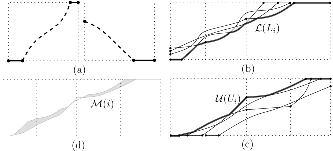
Figure 3: (a) How to extend $B(i,j)$ (dashed line) to $\beta(i,j)$ by attaching horizontal segments (solid line); (b) $\mathcal{L}(L_{i})$, (c) $\mathcal{U}(U_{i})$, and (d) the region $\mathcal{M}(i)$ between them. Here, the dotted boxes are grid cells whose union is $\mathcal{C}_{i}$ and the $s$-axis appears vertical.

Let $\beta(i,j)^{+}\subseteq\mathcal{C}_{i}\cap\mathcal{C}_{j}$ be the region above $\beta(i,j)$ and $\beta(i,j)^{-}$ be the region below $\beta(i,j)$. For a fixed $i$ with $1\leq i\leq 2n$, we classify the $\beta(i,j)$ into two sets $L_{i}$ and $U_{i}$ such that $\beta(i,j)\in L_{i}$ if $R(j,i)=\beta(i,j)^{+}$ or $\beta(i,j)\in U_{i}$ if $R(j,i)=\beta(i,j)^{-}$. Recall that $\mathcal{M}(i)=\mathcal{C}_{i}\setminus\bigcup_{j}R(j,i)$. Thus, we have

$$\mathcal{M}(i)=\mathcal{C}_{i}\setminus\left(\bigcup_{\beta\in L_{i}}\beta^{+}\cup\bigcup_{\beta\in U_{i}}\beta^{-}\right).$$

The boundary of $\bigcup_{\beta\in L_{i}}\beta^{+}$ in $\mathcal{C}_{i}$ is the lower envelope $\mathcal{L}(L_{i})$ of $L_{i}$; symmetrically, the boundary of $\bigcup_{\beta\in U_{i}}\beta^{-}$ in $\mathcal{C}_{i}$ is the upper envelope $\mathcal{U}(U_{i})$ of $U_{i}$. Therefore, $\mathcal{M}(i)=\mathcal{L}(L_{i})^{-}\cap\mathcal{U}(U_{i})^{+}$, the region below the lower envelope $\mathcal{L}(L_{i})$ of $L_{i}$ and above the upper envelope $\mathcal{U}(U_{i})$ of $U_{i}$, and it can be obtained by computing the overlay of two envelopes $\mathcal{L}(L_{i})$ and $\mathcal{U}(U_{i})$. See Figure 3(b)–(d). We exploit known results on the Davenport-Schinzel sequences to obtain the following lemma [19, 12].

Lemma 5

The set $\mathcal{M}(i)$ is of combinatorial complexity $O(\lambda_{66}(n))$ and can be computed in $O(\lambda_{65}(n)\log n)$ time, where $\lambda_{m}(n)$ is the maximum length of a Davenport-Schinzel sequence of order $m$ on $n$ symbols.

• $\beta(i,j)$ consists of at most three arcs, at most one algebraic curve of degree $8$ and at most two straight segments. Thus, we have at most $6n$ algebraic arcs of degree at most $8$. Any two such arcs can intersect each other at most $64$ times by Bézout’s Theorem [11]. Thus, each of $\mathcal{L}(L_{i})$ and $\mathcal{U}(U_{i})$ has complexity $O(\lambda_{66}(n))$ and can be computed in $O(\lambda_{65}(n)\log n)$ time [19, 12].

  After sorting the vertices on these envelopes in $t$-increasing order, we can easily specify all intersections between $\mathcal{L}(L_{i})$ and $\mathcal{U}(U_{i})$ in the same bound.

It should be noted here that the exact constant $66$ is not relevant; it only matters that this is some constant.

We can compute the minimization diagram $\mathcal{M}$ by computing each $\mathcal{M}(i)$ in $O(n\lambda_{65}(n)\log n)$ time. In the same time bound, we can build a point location structure on $\mathcal{M}$. Finally, we conclude our main theorem.

Theorem 2

One can preprocess a given polygonal domain $\mathcal{P}$ in $O(n^{4}\lambda_{65}(n)\log n)$ time into a data structure of size $O(n^{4}\lambda_{66}(n))$ that answers the two-point shortest path query restricted on the boundary $\partial\mathcal{P}$ in $O(\log n)$ time.

4 Tradeoffs Between Space and Query Time

In this section, we provide a space/query-time tradeoff. We use the technique of partitioning $V$, which has been introduced in Chiang and Mitchell [6].

Let $\delta$ be a positive number with $0<\delta\leq 1$. We partition the corner set $V$ into $m=n^{1-\delta}$ subsets $V_{1},\ldots,V_{m}$ of near equal size $O(n^{\delta})$. For each such subset $V_{i}$ of corners, we run the algorithm described above with little modification: We build the shortest path maps $SPM(u)$ only for $u\in V_{i}$ and care about only $O(n^{1+\delta})$ breakpoints induced by such $SPM(u)$. Thus, we consider only the paths from $p(s)$ via $u\in V_{i}$ and $v\in V$ to $p(t)$, and thus $O(n^{1+\delta})$ functions $f_{u,v}$ for $u\in V_{i}$ and $v\in V$.

Since we deal with less number of functions, the cost of preprocessing reduces from $O(n)$ to $O(n^{\delta})$ at several places. We take blocks of $O(n^{\delta})$ grid cells contained in $\mathcal{D}$ and the number of such blocks is $O(n^{2+\delta})$. For each such block, we spend $O(n^{\delta}\lambda_{65}(n^{\delta})\log n)$ time to construct a point location structure for the minimization map $\mathcal{M}_{i}$ of the functions. Iterating all such blocks, we get running time $O(n^{2+2\delta}\lambda_{65}(n^{\delta})\log n)$ for a part $V_{i}$ of $V$. Repeating this for all such subsets $V_{i}$ yields $O(n^{3+\delta}\lambda_{65}(n^{\delta})\log n)$ construction time.

Each query is processed by a series of $m$ point locations on every $\mathcal{M}_{i}$, taking $O(m\log n)=O(n^{1-\delta}\log n)$ time.

Theorem 3

Let $\delta$ be a fixed parameter with $0<\delta\leq 1$. Using $O(n^{3+\delta}\lambda_{65}(n^{\delta})\log n)$ time and $O(n^{3+\delta}\lambda_{66}(n^{\delta}))$ space, one can compute a data structure for $O(n^{1-\delta}\log n)$-time two-point shortest path queries restricted on the boundary $\partial\mathcal{P}$.

Remark that when $\delta=1$, we obtain Theorem 2, and that $O(n^{3+\epsilon})$ time and space is enough for sublinear time query. Note that if $O(n)$ time is allowed for processing each query, $O(n^{2})$ space and $O(n^{2}\log n)$ preprocessing time is sufficient.

5 Extensions to Segments-Restricted Queries

Our approach easily extends to the two-point queries in which queried points are restricted to be on a given segment or a given polygonal chain lying in the free space $\mathcal{P}$.

Let $\mathcal{S}_{s}$ and $\mathcal{S}_{t}$ be two sets of $m_{s}$ and $m_{t}$ line segments, respectively, within $\mathcal{P}$. In this section, we restrict a query pair $(p,q)$ of points to lie on $\mathcal{S}_{s}$ and $\mathcal{S}_{t}$ each. We will refer to this type of two-point query as a $(\mathcal{S}_{s},\mathcal{S}_{t})$-restricted two-point query. As we did above, we take two segments $S\in\mathcal{S}_{s}$ and $T\in\mathcal{S}_{t}$ and let $b_{S}$ and $b_{T}$ be the number of breakpoints — the intersection points with an edge of $SPM(v)$ for some $v\in V$ — on $S$ and $T$, respectively. Also, parameterize $S$ and $T$ as above so that we have two bijections $p:[0,|S|]\to S$ and $q:[0,|T|]\to T$.

Any path from a point on $S$ leaves to one of the two sides of $S$. Thus, the idea of handling such a segment within the free space $\mathcal{P}$ is to consider two cases separately. Here, we regard $S$ and $T$ as directed segments in direction of movement of $p(s)$ and $q(t)$ as $s$ and $t$ increases, and consider only one case where paths leave $S$ to its left side and arrive at $T$ from its left side. The other cases are analogous.

Then, the situation is almost identical to that we considered in Section 3.2. For a pair of segments $S$ and $T$, we can construct a query structure in $O(b_{S}\lceil\frac{b_{T}}{n}\rceil n\lambda_{65}(n)\log n)$ time. Unfortunately, $b_{S}$ and $b_{T}$ can be as large as $O(n^{2})$, yielding the same time bound for $(\partial\mathcal{P},\partial\mathcal{P})$-restricted two-point queries in the worst case. Thus, in the worst case, we need additional factor of $m_{s}m_{t}$ as follows.

Theorem 4

Let $\mathcal{S}_{s}$ and $\mathcal{S}_{t}$ be two sets of $m_{s}$ and $m_{t}$ (possibly crossing) line segments, respectively, within $\mathcal{P}$, and $\delta$ be a fixed parameter with $0<\delta\leq 1$. Then, using $O(m_{s}m_{t}n^{3+\delta}\lambda_{65}(n^{\delta})\log n)$ time and $O(m_{s}m_{t}n^{3+\delta}\lambda_{66}(n^{\delta}))$ space, one can compute a data structure for $O(n^{1-\delta}\log(n+m_{s}+m_{t}))$-time $(\mathcal{S}_{s},\mathcal{S}_{t})$-restricted two-point queries.

Remark that in practice we expect that the number of breakpoints $\sum_{S}b_{S}$ and $\sum_{T}b_{T}$ is not so large as $\Omega(n^{2})$ that the preprocessing and required storage would be much less than the worst case bounds.

6 Concluding Remarks

In this paper, we posed the variation of the two-points query problem in polygonal domains where the query points are restricted in a specified subset of the free space. And we obtained significantly better bounds for the boundary-restricted two-point queries than for the general queries.

Despite of its importance, the two-point shortest path query problem for the polygonal domains is not well understood. There is a huge gap ($O(n)$ to $O(n^{11})$) about logarithmic query between the simple polygon case and the general case but still the reason why we need such a large storage is still unclear. On the other hand, restriction on the query domain provides another possibility of narrowing the gap with several new open problems: (1) What is the right upper bound on the complexity of the lower envelope defined by the functions $f_{u,v}$ on the parameterized query domain? And what about any lower bound construction? (2) If the query domain is a simple $2$-dimensional shape, such as a triangle, then can one achieve a better performance than the general results by Chiang and Mitchell?

We would carefully conjecture that our upper bound $\tilde{O}(n^{5})$ for logarithmic query could be improved to $\tilde{O}(n^{4})$. Indeed, we have $O(n^{4})$ grid cells on the parameterized query domain and whenever we cross their boundaries, changes in the involved functions are usually bounded by a constant amount. Thus, if one could find a clever way of updating the functions and their lower envelope, it would be possible to achieve an improved bound.

References

- [1] P. K. Agarwal, B. Aronov, J. O’Rourke, and C. A. Schevon. Star unfolding of a polytope with applications. SIAM J. Comput., 26(6):1689–1713, 1997.
- [2] P. K. Agarwal, B. Aronov, and M. Sharir. Computing envelopes in four dimensions with applications. SIAM J. Comput., 26(6):1714–1732, 1997.
- [3] P. K. Agarwal and M. Sharir. Arrangements and their applications. In J.-R. Sack and J. Urrutia, editors, Handbook of Computationaal Geometry, pages 49–119. Elsevier Science Publishers B.V., 2000.
- [4] S. R. Arikati, D. Z. Chen, L. P. Chew, G. Das, M. H. M. Smid, and C. D. Zaroliagis. Planar spanners and approximate shortest path queries among obstacles in the plane. In Proc. 4th Annu. Euro. Sympos. Algo. (ESA’96), pages 514–528, 1996.
- [5] D. Z. Chen. On the all-pairs Euclidean short path problem. In SODA ’95: Proceedings of the sixth annual ACM-SIAM symposium on Discrete algorithms, pages 292–301, 1995.
- [6] Y.-J. Chiang and J. S. B. Mitchell. Two-point Euclidean shortest path queries in the plane. In Proc. 10th ACM-SIAM Sympos. Discrete Algorithms (SODA), pages 215–224, 1999.
- [7] K. Clarkson. Approximation algorithms for shortest path motion planning. In Proc. 19th ACM Sympos. Theory Comput. (STOC ’87), pages 56–65, 1987.
- [8] A. F. Cook IV and C. Wenk. Shortest path problems on a polyhedral surface. In Proc. 11th Intern. Sympos. Algo. Data Struct. (WADS’09), pages 156–167, 2009.
- [9] L. J. Guibas and J. Hershberger. Optimal shortest path queries in a simple polygon. J. Comput. Syst. Sci., 39(2):126–152, 1989.
- [10] H. Guo, A. Maheshwari, and J.-R. Sack. Shortest path queries in polygonal domains. In AAIM, pages 200–211, 2008.
- [11] R. Hartshorne. Algebraic Geometry. Springer, 1977.
- [12] J. Hershberger. Finding the upper envelope of line segments in time. Inf. Process. Lett., 33(4):169–174, 1989.
- [13] J. Hershberger and S. Suri. An optimal algorithm for Euclidean shortest paths in the plane. SIAM J. Comput., 28(6):2215–2256, 1999.
- [14] J. S. B. Mitchell. Shortest paths among obstacles in the plane. Internat. J. Comput. Geom. Appl., 6(3):309–331, 1996.
- [15] J. S. B. Mitchell. Shortest paths and networks. In Handbook of Discrete and Computational Geometry, chapter 27, pages 607–641. CRC Press, Inc., 2nd edition, 2004.
- [16] G. Nivasch. Improved bounds and new techniques for Davenport-Schinzel sequences and their generatlizations. In Proc. 20th ACM-SIAM Sympos. Discrete Algorithms, pages 1–10, 2009.
- [17] J. O’Rourke and S. Suri. Polygons. In Handbook of discrete and computational geometry, chapter 26, pages 583–606. CRC Press, Inc., Boca Raton, FL, USA, 2nd edition, 2004.
- [18] M. Sharir. Almost tight upper bounds for lower envelopes in higher dimensions. Discrete Comput. Geom., 12:327–345, 1994.
- [19] M. Sharir and P. K. Agarwal. Davenport-Schinzel Sequences and Their Geometric Applications. Cambridge University Press, New York, 1995.