Collective fluctuations in networks of noisy components

Abstract

Collective dynamics result from interactions among noisy dynamical components. Examples include heartbeats, circadian rhythms, and various pattern formations. Because of noise in each component, collective dynamics inevitably involve fluctuations, which may crucially affect functioning of the system. However, the relation between the fluctuations in isolated individual components and those in collective dynamics is unclear. Here we study a linear dynamical system of networked components subjected to independent Gaussian noise and analytically show that the connectivity of networks determines the intensity of fluctuations in the collective dynamics. Remarkably, in general directed networks including scale-free networks, the fluctuations decrease more slowly with the system size than the standard law stated by the central limit theorem. They even remain finite for a large system size when global directionality of the network exists. Moreover, such nontrivial behavior appears even in undirected networks when nonlinear dynamical systems are considered. We demonstrate it with a coupled oscillator system.

1 Introduction

Understanding fluctuations in dynamically ordered states and physical objects, which consist of networks of interacting components, is an important issue in many disciplines ranging from biology to engineering. When each constituent component of a system is noisy due to, e.g., thermal fluctuations, it generally occurs that the entire system collectively fluctuates in time. Such collective fluctuations may be advantageous or disadvantageous in functioning of the systems depending on situations. For example, reduction in noise is likely to improve information processing in retinal neural networks [1, 2, 3, 4]. Precision of biological circadian clocks [5, 6, 7, 8] may be improved by reduction in collective fluctuations (i.e., fluctuations in collective activities). On the other hand, maintaining a certain amount of fluctuations in an ordered state is advantageous for stochastic resonance [9] and Brownian motors [10].

Despite the relevance of collective fluctuations in a variety of systems, theoretical frameworks that formulate collective fluctuations are missing. The central limit theorem states that, if the dynamical order is simply the averaged activity of noisy components, the standard deviation of the collective fluctuation would decrease with the number $N$ of noisy components as $N^{-1/2}$. However, scaling is unclear in systems of interacting components. Clarifying the property of collective fluctuations in such systems will give us insights into the mechanisms and design principles underlying the regulation of noise in, for example, living organisms and chemical reactions, and also into possible controls of fluctuations in collective dynamics.

In this study, we analyze an ensemble of components subjected to independent Gaussian noise that interact on general networks, including complex networks and regular lattices. We first consider a linear dynamical system, which can be regarded as linearization of various systems, such as networks of periodic or chaotic oscillators [11, 12], the overdamped limit of elastic networks [13], a consensus problem treated in control theory [14]. We show that collective fluctuations are determined by the connectivity of networks. It turns out that the scaling $N^{-1/2}$ is the tight lower bound, which is obtained for undirected networks. General directed networks yield a slower or nonvanishing decay of collective fluctuations with an increase in $N$. We then argue such nontrivial behavior appears even in undirected networks when nonlinear systems are considered. In particular, we show that linearization of coupled nonlinear oscillator systems on undirected media yields linear dynamics on asymmetric networks, such that the slow decay of the collective fluctuation is relevant.

2 Model and analysis

Consider a network of $N$ components obeying

$$\dot{x}_{i}=\sum_{j=1}^{N}w_{ij}(x_{j}-x_{i})+\sqrt{D_{i}}\xi_{i}(t),\quad(1\leq i\leq N),$$ (1)

where $x_{i}$ is the state (or the position) of the $i$th component, $\sqrt{D_{i}}$ is the intensity of noise, $\xi_{i}$ is the independent Gaussian (generally colored) noise, and $w_{ij}$ is the intensity of coupling and can be also regarded as originating from the Jacobian matrix of underlying nonlinear dynamical systems such as coupled oscillator systems that we consider later. We allow negative weights and asymmetric coupling; $w_{ij}$ can be negative or different from $w_{ji}$. Equation (1) is a multivariate Ornstein-Uhlenbeck process [15, 16].

For convenience, we represent Eq. (1) as

$$\dot{\bm{x}}=-L\bm{x}+\bm{p},$$ (2)

where ${\bm{x}}\equiv(x_{1}\;\ldots\;x_{N})^{\top}$ ($\top$ denotes the transpose), $\bm{p}\equiv(\sqrt{D_{1}}\xi_{1}\;\ldots\;\sqrt{D_{N}}\xi_{N})^{\top}$, and $L=(L_{ij})$ is the asymmetric Laplacian defined by $L_{ij}=\delta_{ij}\sum_{i^{\prime}\neq i}w_{ii^{\prime}}-(1-\delta_{ij})w_{ij}$ [17, 18]. $L$ always has a zero eigenvalue with the right eigenvector $\bm{u}\equiv(1\;\ldots\;1)^{\top}$, i.e., $L\bm{u}=0$. This eigenvector is associated with a global translational shift in state $\bm{x}$ and corresponds to the fact that such a shift keeps Eq. (1) invariant. We assume the stability of the ordered state represented by $x_{1}=\ldots=x_{N}$ in the absence of the noise (i.e., $D_{i}=0$ for all $i$); the system relaxes to the ordered state from any initial condition. This is equivalent to assuming that the real parts of all the eigenvalues of $L$ are positive except for one zero eigenvalue, i.e., $0\equiv\lambda_{1}<{\rm Re}\lambda_{2}\leq\ldots\leq{\rm Re}\lambda_{N}$. This is a nontrivial condition for general networks with negative weights. However, for networks with only non-negative weights, i.e., $w_{ij}\geq 0$ ($1\leq i,j\leq N$), this property holds true when the network is strongly connected or all the nodes are reachable by a directed path from a single node [19, 20, 17].

We are concerned with collective fluctuations in dynamics given by Eq. (1). To quantify their intensity, we decompose $\bm{x}$ as

$$\bm{x}(t)=y(t)\bm{u}+\bm{\rho}(t).$$ (3)

$y(t)$ describes the one-dimensional component along $\bm{u}$, and $\bm{\rho}(t)$ is the ($N-1$)-dimensional remainder mode. Note that $y(t)=\bm{v}\bm{x}(t)$, where the row vector $\bm{v}\equiv(v_{1}\ldots v_{N})$ is the left eigenvector of $L$ corresponding to the zero eigenvalue, i.e., $\bm{v}L=0$, and is normalized as $\bm{v}\bm{u}=1$, i.e., $\sum_{i=1}^{N}v_{i}=1$ (see Appendix A for detailed descriptions). We call $y(t)\bm{u}$ the collective mode. In the absence of noise, the dynamical equation for $y(t)$ is given by

$$\dot{y}=\bm{v}\dot{\bm{x}}=-\bm{v}L\bm{x}=0.$$ (4)

Therefore, $y(t)$ is a conserved quantity of the dynamics. The remainder mode $\bm{\rho}(t)$ is associated with relative motions among the components. Because of the stability assumption, $\bm{\rho}(t)$ asymptotically vanishes with characteristic time $({\rm Re}~{}\lambda_{2})^{-1}$. Therefore, all the values of $x_{i}$ ($1\leq i\leq N$) eventually go to the same value $y$ that is determined by the initial condition, i.e., $y=\bm{v}\bm{x}(0)$.

In the presence of noise, we obtain

$$\dot{y}=\bm{v}\dot{\bm{x}}=\bm{v}(-L\bm{x}+\bm{p})=\bm{v}\bm{p}=\sum_{i=1}^{N}v_{i}\sqrt{D_{i}}\xi_{i}(t).$$ (5)

Because $\xi_{i}$ is the independent Gaussian noise, this equation reduces to

$$\dot{y}(t)=\sqrt{\sum_{i=1}^{N}v_{i}^{2}D_{i}}\xi(t)\equiv\sigma\xi(t),$$ (6)

where $\xi(t)$ is the Gaussian noise having the same statistical property as that of each $\xi_{i}(t)$. Thus, $y(t)$ performs the Brownian motion with effective noise strength $\sigma$ and is unbounded. The remainder mode $\bm{\rho}(t)$ fluctuates around zero because of its decaying nature. Therefore, the long-time behavior of $x_{i}(t)=y(t)+\rho_{i}(t)$ is approximately described by a single variable $y(t)$ for any $i$. We denote as $\sigma$, which depends on the structure of the network, the intensity of collective fluctuations. $\sigma$ can be calculated for given network.

In practice, the average activity of the population, $\bar{x}\equiv\sum_{i=1}^{N}x_{i}/N$, but not the activity at individual nodes, may be observed. Because $\bar{x}=y+\sum_{i=1}^{N}\rho_{i}/N$ and $\sum_{i=1}^{N}\rho_{i}/N$ can be neglected in a long run, $\sigma$ also characterizes the fluctuations of $\bar{x}$.

3 Collective fluctuations in various networks

3.1 General properties

We assume for simplicity that $D_{i}=1$ ($1\leq i\leq N$) so that $\sigma=\sqrt{\sum_{i=1}^{N}v_{i}^{2}}$. It is straightforward to extend the following results to the case of heterogeneous $D_{i}$. The vector $\bm{v}$ is uniform, i.e., $v_{i}=1/N$ ($1\leq i\leq N$) if and only if $k_{i}^{\rm in}=k_{i}^{\rm out}$ ($1\leq i\leq N$), where $k_{i}^{\rm in}\equiv\sum_{j=1}^{N}w_{ij}$ and $k_{i}^{\rm out}\equiv\sum_{j=1}^{N}w_{ji}$ are indegree and outdegree, respectively [18]. Undirected networks satisfy this condition. In this case, we obtain $\sigma=N^{-1/2}$, which agrees with the central limit theorem. The normalization condition $\sum_{i=1}^{N}v_{i}=1$ guarantees that $\sigma\geq N^{-1/2}$ for any $\bm{v}$. Therefore, undirected networks are the best for reducing collective fluctuations. In the case of directed or asymmetrically weighted networks, $v_{i}$ is generally heterogeneous, and $\sigma>N^{-1/2}$. We will show later that this is also the case for nonlinear systems on undirected networks. When the weight $w_{ij}$ is nonnegative for any $i$ and $j$, the Perron–Frobenius theorem guarantees that $v_{i}$ is nonnegative for all $i$ [21]. In this case, we obtain

$$\frac{1}{\sqrt{N}}\leq\sigma\leq 1.$$ (7)

The case $\sigma=1$ is realized by a feedforward network, in which a certain component $i_{0}$ has no inward connection (i.e., $k_{i_{0}}^{\rm in}=0$). Then, $v_{i_{0}}=1$ and $v_{i}=0$ for $i\neq i_{0}$, which yields $\sigma=1$ irrespective of $N$; the collective fluctuations are not reduced at all with an increase in $N$. When negative weights are allowed, some elements of $\bm{v}$ may assume negative values. Then, $\sigma$ may be larger than $1$, in which case collective fluctuations are larger than individual noise.

We note that $\sigma^{2}$ is the so-called inverse participation ratio [22]. $\sigma^{-2}$ can be interpreted as the effective number of components that participate in collective activities; the remaining components are slaved.

3.2 Directed scale-free networks

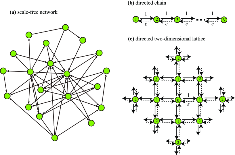
Figure 1: Schematic of (a) directed scale-free network, (b) directed chain, and (c) directed two-dimensional lattice. The numbers in (b) indicate the indices of the nodes, while those in (c) indicate the layer index.

We demonstrate our theory by using some example networks. First, we consider directed scale-free networks, schematically shown in Fig. 1(a) in which $k_{i}^{\rm in}$ and $k_{i}^{\rm out}$ independently follow the distributions $p(k^{\rm in})\propto k^{-\gamma_{\rm in}}$ and $p(k^{\rm out})\propto k^{-\gamma_{\rm out}}$, respectively. By assuming that the values of $v_{i}$ of adjacent nodes are independent of each other, we obtain

$$\sum_{j=1}^{N}w_{ji}v_{j}\approx\sum_{j=1}^{N}w_{ji}\bar{v}=k_{i}^{\rm out}\bar{v},$$ (8)

where

$$\bar{v}\equiv\frac{\sum^{N}_{i=1}v_{i}}{N}=\frac{1}{N}.$$ (9)

Therefore,

$$v_{i}=\frac{\sum_{j=1}^{N}w_{ji}v_{j}}{\sum_{j=1}^{N}w_{ij}}\approx\frac{k_{i}^{\rm out}/k_{i}^{\rm in}}{\sum_{j=1}^{N}\left(k_{j}^{\rm out}/k_{j}^{\rm in}\right)}.$$ (10)

This approximation is sufficiently accurate for uncorrelated networks [18]. For $p(k^{\rm in})\propto k^{-\gamma_{\rm in}}$ and $p(k^{\rm out})\propto k^{-\gamma_{\rm out}}$, we obtain

$$v_{i}\approx\frac{k_{i}^{\rm out}/k_{i}^{\rm in}}{N\left<k^{\rm out}\right>\left<(k^{\rm in})^{-1}\right>}$$ (11)

and

$$\sigma\approx\sqrt{\frac{\left<\left(k^{\rm out}\right)^{2}\right>\left<\left(k^{\rm in}\right)^{-2}\right>}{N\left<k^{\rm out}\right>^{2}\left<\left(k^{\rm in}\right)^{-1}\right>^{2}}},$$ (12)

where $\left<\cdot\right>$ is the ensemble average. When $\gamma_{\rm out}<2$, a winner-take-all network is generated [23, 24], and there exists a node $i$ such that $k_{i}^{\rm out}=O(N)$ and $v_{i}=O(1)$. When $\gamma_{\rm out}\geq 2$, the extremal criterion results in the maximum degree increasing with $N$ as $N^{1/(\gamma_{\rm out}-1)}$ ($\gamma_{\rm out}\geq 2$) in many networks [25, 24]. Then, we obtain [26]

$$\left<k^{\rm out}\right>\propto\left\{\begin{array}[]{ll}N^{2-\gamma_{\rm out}},&(\gamma_{\rm out}<2),\\ \ln N,&(\gamma_{\rm out}=2),\\ O(1),&(\gamma_{\rm out}>2),\end{array}\right.$$ (13)

$$\left<\left(k^{\rm out}\right)^{2}\right>\propto\left\{\begin{array}[]{ll}N^{-\gamma_{\rm out}+3},&(\gamma_{\rm out}<2),\\ N^{(-\gamma_{\rm out}+3)/(\gamma_{\rm out}-1)},&(2\leq\gamma_{\rm out}<3),\\ \ln N,&(\gamma_{\rm out}=3),\\ O(1),&(\gamma_{\rm out}>3),\end{array}\right.$$ (14)

and

$$\left<\left(k^{\rm in}\right)^{-1}\right>,\left<\left(k^{\rm in}\right)^{-2}\right>=O(1).$$ (15)

Therefore, we obtain

$$\sigma\propto\left\{\begin{array}[]{ll}1,&(\gamma_{\rm out}<2),\\ 1/\ln N,&(\gamma_{\rm out}=2),\\ N^{-1+(\gamma_{\rm out}-1)^{-1}},&(2\leq\gamma_{\rm out}<3),\\ N^{-1/2}(\ln N)^{1/2},&(\gamma_{\rm out}=3),\\ N^{-1/2},&(\gamma_{\rm out}>3).\end{array}\right.$$ (16)

The fairly heterogeneous case $\gamma_{\rm out}<2$, in which the average outdegree diverges as $N\to\infty$, effectively yields a feedforward network. The case $\gamma_{\rm out}\geq 3$, where the second moment of the outdegree converges for $N\to\infty$, reproduces the central limit theorem. The latter result is shared by the directed version of the conventional random graph. The case $2\leq\gamma_{\rm out}<3$ yields a nontrivial dependence of $\sigma$ on $N$. In Fig. 2(a), we compare the scaling exponent $\beta$, where $\sigma\propto N^{-\beta}$ obtained from the theory (solid line; Eq. (16)) and numerical simulations of the configuration model [27, 23] with the power-law degree distribution with minimum degree 3 (open circles). The fitting procedure is explained in Fig. 2(b). Equation (16) roughly explains numerically obtained values of $\beta$.

3.3 Directed lattices

The second example is the directed one-dimensional chain of $N$ nodes depicted in Fig. 1(b). We set $w_{i+1,i}=1$ ($1\leq i\leq N-1$), $w_{i-1,i}=\epsilon$ ($2\leq i\leq N$), and $w_{j,i}=0$ ($j\neq i-1,i+1$). For this network, by solving $\bm{v}L=0$, we analytically obtain

$$v_{i}=\frac{(1-\epsilon)\epsilon^{i-1}}{1-\epsilon^{N}},\quad(1\leq i\leq N)$$ (17)

and

$$\sigma=\sqrt{\frac{1-\epsilon}{1+\epsilon}\,\frac{1+\epsilon^{N}}{1-\epsilon^{N}}}.$$ (18)

Values of $\sigma$ for various $\epsilon$ and $N$ are plotted by solid lines in Fig. 3(a). Interestingly, for $\epsilon\neq 1$, $\lim_{N\to\infty}\sigma=\sqrt{(1-\epsilon)/(1+\epsilon)}$; $\sigma$ is nonvanishing. We have also analytically derived $\sigma$ for directed $d$-dimensional lattices (see Appendix B). The results for the two-dimensional lattice depicted in Fig. 1(c) are plotted by solid lines in Fig. 3(b). To confirm our theory, we also carried out direct numerical simulations of Eq. (1) with Gaussian white noise for these directed lattices. The results indicated by circles in Fig. 3 indicate an excellent agreement with our theory.

A similar result is obtained for the Cayley tree (see Appendix C).

4 Oscillator dynamics

As an application of our theory to nonlinear systems, we examine noisy and rhythmic components. As a general, tractable, yet realistic model, we consider a network of phase oscillators [28, 11, 29], whose dynamical equation is given by

$$\dot{\phi}_{i}=\omega_{i}+\sum_{j=1}^{N}A_{ij}f(\phi_{j}-\phi_{i})+\sqrt{D_{i}}\xi_{i}(t),\quad(1\leq i\leq N),$$ (19)

where $\phi_{i}\in[0,2\pi)$ and $\omega_{i}$ are the phase and the intrinsic frequency of the $i$th oscillator, respectively, $A_{ij}$ is the intensity of coupling, and $f(\cdot)$ is a $2\pi$–periodic function. We assume that, in the absence of noise, all the oscillators are in a fully phase-locked state, i.e., $\phi_{i}(t)=\Omega t+\psi_{i}$, where $\Omega$ and $\psi_{i}$ are the constants derived from $\dot{\phi}_{i}=\Omega$ ($1\leq i\leq N$). Under sufficiently weak noise, we can linearize Eq. (19) around the phase-locked state. Letting $x_{i}=\phi_{i}-(\psi_{i}+\Omega t)$, we obtain Eq. (1), where $w_{ij}=A_{ij}f^{\prime}(\psi_{j}-\psi_{i})$ is the effective weight. The validity of linearizing Eq. (19) for small noise intensity is tested by carrying out direct numerical simulations of Eq. (19) with $\omega_{i}=\omega$ ($1\leq i\leq N$) and $f(\phi)=\sin\phi$. The relationship $\sigma\approx\sqrt{\sum_{i=1}^{N}D_{i}v_{i}^{2}}$ is satisfied in the directed one- and two-dimensional lattices, as shown in Fig. 4(a) and (b), respectively.

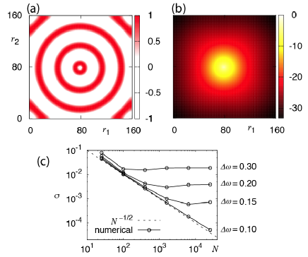
Figure 5: (color online) Numerical results of the coupled oscillators on the two-dimensional undirected lattice. (a) Snapshot of $\sin\phi_{i}$ and (b) eigenvector $\bm{v}$ (log scale) for $\Delta\omega=0.3$, where $r_{1}$ and $r_{2}$ denote the spatial coordinates. (c) The dependence of $\sigma$ on system size $N$.

When there is some dispersion in $\psi_{i}$ in a phase-locked state, the relation $\sigma\approx N^{-1/2}$ may be violated even in undirected networks. This is because the effective weight is generally asymmetric (i.e., $w_{ij}\neq w_{ji}$) unless $f(\cdot)$ is an exact odd function. In reality, $f(\cdot)$ is usually not an odd function [11, 30, 31, 29]. As an example, we consider target patterns (i.e., concentric traveling waves), which naturally appear in spatially extended oscillator systems [11, 32]. We carry out direct numerical simulations of Eq. (19) on the two-dimensional undirected lattice with linear length $\sqrt{N}=50$, $f(\phi)=\sin(\phi-\alpha)+\sin\alpha$, and $\alpha=\pi/4$. Such a function may be analytically derived from a general class of coupled oscillators [11], and it approximates a variety of real systems [31, 33, 29]. We set $\omega_{i}=\omega_{0}+\Delta\omega$ $(\Delta\omega\geq 0)$ for $4\times 4$ pacemaker oscillators in the center and $\omega_{i}=\omega_{0}$ for the other oscillators, where $\omega_{0}$ is arbitrary and set to $1$. A target pattern is formed when there is sufficient heterogeneity in the intrinsic frequency [11]. A region with high intrinsic frequency acts as a pacemaker. A snapshot for $\Delta\omega=0.3$ is shown in Fig. 5(a). As observed, the radial phase gradient is approximately constant, which makes the effective network similar to the directed two-dimensional lattice depicted in Fig. 1(c). Therefore, as shown in Fig. 5(b), $v_{i}$ calculated numerically decreases almost exponentially with the distance from the center. We find that the dependence of $\sigma$ on $N$, shown in Fig. 5(c), is similar to that for directed lattices.

We emphasize that the network is undirected (i.e., $A_{ij}=A_{ji}$). We have also theoretically confirmed that our results are valid for the continuous oscillatory media under spatial block noise, which models chemical reaction–diffusion systems (see Appendix D).

5 Conclusions

In summary, we have obtained the analytical relationship between collective fluctuations and the structure of networks. In undirected networks, the fluctuations decrease with the system size $N$ as $N^{-1/2}$; this result agrees with the central limit theorem. In general directed networks, the collective fluctuations decay more slowly. For example, in directed scale-free networks, we obtain $N^{-\beta}$ with $0<\beta<1/2$. In networks with global directionality, the fluctuations do not vanish for a large system size. We have also demonstrated that such nontrivial dependence appears even in undirected networks when nonlinear systems are considered. We have focused on systems of nonleaky components. Results for coupled leaky components will be reported elsewhere.

Our results are distinct from earlier results demonstrating the breach of the central limit theorem due to heavy-tailed noise [34] or the correlation between the noise in different elements [35, 36].

Finally, because our theory is based on a general linear model, it can be tested in a variety of experimental systems. An ideal experimental protocol is provided by photo-sensitive Belousov-Zhabotinsky reaction systems, in which the heterogeneity, noise intensity, and system size can be precisely controlled by light stimuli [32]. Experiments with coupled oscillatory cells, such as cardiac cells and neurons under an appropriate condition, would be also interesting.

Appendix A: Derivation of the collective mode

To derive the collective mode $y(t)\bm{u}$, we note that there exists a nonsingular matrix $P$ such that $\tilde{L}\equiv P^{-1}LP$ is its Jordan canonical form [21, 17]. We assume that $\tilde{L}_{11}=\lambda_{1}=0$ and $\tilde{L}_{1i}=\tilde{L}_{i1}=0$ ($2\leq i\leq N$) without loss of generality. The submatrix $(\tilde{L}_{ij})$ ($2\leq i,j\leq N$) corresponds to the $N-1$ modes with the eigenvalues $\lambda_{2},\ldots,\lambda_{N}$. Because the first column of $LP=P\tilde{L}$ is equal to $(0\;\ldots\;0)^{\top}$, the first column of $P$ is equal to the right eigenvector of $L$ corresponding to $\lambda_{1}=0$, i.e., $\bm{u}=(1\;\ldots\;1)^{\top}$. Because the first row of $P^{-1}L=\tilde{L}P^{-1}$ is equal to $(0\;\ldots\;0)$, the first row of $P^{-1}$ is equal to the left eigenvector of $L$ corresponding to $\lambda_{1}=0$, i.e., $\bm{v}=(v_{1}\;v_{2}\;\ldots\;v_{N})$. The normalization is given by $\sum_{i=1}^{N}v_{i}=1$. Under the variable change $(y\;\bm{y}_{\rm r})\equiv P^{-1}\bm{x}\in\mathbb{R}^{N}$, where $y\in\mathbb{R}$ and $\bm{y}_{\rm r}\in\mathbb{R}^{N-1}$, the coupling term is transformed into $-\tilde{L}(y\;\bm{y}_{\rm r})$. Then, in the absence of the dynamical noise, $y=\sum_{i=1}^{N}v_{i}x_{i}$ is a conserved quantity, which is the collective mode. $\bm{\rho}(t)$ in Eq. (3) is given by $P_{\rm r}\bm{y}_{\rm r}$, where $P_{\rm r}$ is the $N$ by $N-1$ matrix satisfying $P=(\bm{u}\;P_{\rm r})$.

Appendix B: Collective fluctuations in regular lattices with arbitrary dimensions

Consider a directed two-dimensional square lattice with a root node. As depicted in Fig. 1(c), the edges descending from the root node and those approaching the root node in terms of the graph-theoretic distance are given weight 1 and $\epsilon$ ($0\leq\epsilon\leq 1$), respectively. We define layers such that the layer $\ell$ ($\leq\ell_{\max}$) is occupied by the nodes whose distance from the root node is equal to $\ell$. Layer 0 contains the root node only, and layer $\ell$ ($\geq 1$) contains $4\ell$ nodes. We consider the lattice within a finite range specified by $\ell\leq\ell_{\max}$. Note the difference from the case of the one-dimensional chain examined in the main text (Fig. 1(b)), where the root node is located at the periphery of the chain. However, the scaling of $\sigma$ is not essentially affected by this difference.

The symmetry guarantees that the four nodes in layer 1 have the same value of $v_{i}$. Consider a node in Fig. 1(c) that is labeled 2 and adjacent to two nodes labeled 1. There are four such nodes. The equation in $\bm{v}L=0$ corresponding to this node is given by $(2+2\epsilon)v_{2}=2\epsilon v_{1}+2v_{3}$. The other four nodes labeled 2 in Fig. 1(c) yield a different equation $(1+3\epsilon)v_{2}=\epsilon v_{1}+3v_{3}$. Similarly, we obtain $(2+2\epsilon)v_{\ell}=2\epsilon v_{\ell-1}+2v_{\ell+1}$ for all but four nodes in layer $\ell$. The other four nodes satisfy $(1+3\epsilon)v_{\ell}=\epsilon v_{\ell-1}+3v_{\ell+1}$. Despite this inhomogeneity, $v_{\ell}\propto\epsilon^{\ell}$ satisfies all these equations. By counting the number of nodes in each layer, the properly normalized solution is given by

$$v_{\ell}=\left[T_{\ell_{\max}}^{(2)}(\epsilon)\right]^{-1}\,\epsilon^{\ell},\qquad(0\leq\ell\leq\ell_{\max}),$$ (S.20)

and

$$\sigma=\frac{\sqrt{T_{\ell_{\max}}^{(2)}(\epsilon^{2})}}{T_{\ell_{\max}}^{(2)}(\epsilon)},$$ (S.21)

where

$$T_{\ell_{\max}}^{(2)}(z) = 1+4\sum_{\ell=1}^{\ell_{\max}}\ell z^{\ell}$$ (S.22)

$$= \frac{(1+z)^{2}-4[1+{\ell_{\max}}(1-z)]z^{\ell_{\max}+1}}{(1-z)^{2}}.$$

The difference between the one- and two-dimensional cases lies in the number of nodes in each layer, which affects the normalization of $v_{\ell}$ and hence the value of $\sigma$. In the limit of a purely feedforward network, $\sigma$ is independent of the system size, i.e., $\lim_{\epsilon\to 0}\sigma=1$. In the case of undirected networks, the central limit theorem is recovered, i.e., $\lim_{\epsilon\to 1}\sigma=N^{-1/2}$. In the limit of infinite space, we obtain

$$\lim_{{\ell_{\max}}\to\infty}\sigma=\frac{(1-\epsilon)(1+\epsilon^{2})}{(1+\epsilon)^{3}}.$$ (S.23)

For a general dimension $d$, layer 0 has a single root node, and layer $\ell$ ($1\leq\ell\leq\ell_{\max}$) has

$$N_{\ell}^{(d)}\equiv\sum_{d^{\prime}=1}^{\ell}\frac{d!}{d^{\prime}!(d-d^{\prime})!}\frac{(\ell-1)!}{(d^{\prime}-1)!(\ell-d^{\prime})!}2^{d^{\prime}}$$

nodes. $d^{\prime}$ is the number of coordinates among the $d$ coordinates to which nonzero values are assigned, and the factor $2^{d^{\prime}}$ takes care of the fact that reversing the sign of any coordinate does not change the layer of the node. Similar to the case of the two-dimensional lattice, the value of $v_{i}$ for any node in layer $\ell$ in a $d$-dimensional lattice, denoted by $v_{\ell}^{(d)}$, is given by

$$v_{\ell}^{(d)}=\left[T_{\ell_{\max}}^{(d)}(\epsilon)\right]^{-1}\,\epsilon^{\ell},\qquad(0\leq\ell\leq\ell_{\max}),$$ (S.24)

where

$$T_{\ell_{\max}}^{(d)}(z)=1+\sum_{\ell=1}^{\ell_{\max}}N_{\ell}^{(d)}z^{\ell}$$ (S.25)

From Eq. (S.24), we obtain

$$\sigma=\frac{\sqrt{T_{\ell_{\max}}^{(d)}(\epsilon^{2})}}{T_{\ell_{\max}}^{(d)}(\epsilon)}.$$ (S.26)

Note that $\lim_{\epsilon\to 0}\sigma=1$ and $\lim_{\epsilon\to 1}\sigma=N^{-1/2}$. In the limit $\ell_{\max}\to\infty$, Eq. (S.25) becomes

$$\lim_{\ell_{\max}\to\infty}T_{\ell_{\max}}^{(d)}(z) = 1+\sum_{d^{\prime}=1}^{\infty}\frac{d!}{d^{\prime}!(d-d^{\prime})!}2^{d^{\prime}}\sum_{\ell=d^{\prime}}^{\infty}\frac{(\ell-1)!}{(d^{\prime}-1)!(\ell-d^{\prime})!}z^{\ell}$$ (S.27)

$$= 1+\sum_{d^{\prime}=1}^{\infty}\frac{d!}{d^{\prime}!(d-d^{\prime})!}2^{d^{\prime}}\left(\frac{z}{1-z}\right)^{d^{\prime}}$$

$$= \left(\frac{1+z}{1-z}\right)^{d}.$$

Substituting Eq. (S.27) into Eq. (S.26) yields

$$\lim_{\ell_{\max}\to\infty}\sigma=\left[\frac{\left(1-\epsilon\right)\left(1+\epsilon^{2}\right)}{\left(1+\epsilon\right)^{3}}\right]^{d/2}.$$ (S.28)

Appendix C: Collective fluctuations in the Cayley tree

Consider a Cayley tree with degree $k$ and a specific root node. We assume that the maximum distance from the root node is equal to $\ell_{\max}$. The edges descending from the root node and those approaching the root node are assigned weight 1 and $\epsilon$, respectively. The exact value of $v_{i}$ in layer $\ell$, denoted by $v_{\ell}$ without confusion, is obtained via

$$\left[1+\left(k-1\right)\epsilon\right]v_{\ell}=\epsilon v_{\ell-1}+\left(k-1\right)v_{\ell+1},\quad(\ell\geq 1).$$ (S.29)

By solving Eq. (S.29), we obtain

$$v_{\ell}=\frac{1-(\epsilon k)}{1-(\epsilon k)^{\ell_{\max}+1}}\,\epsilon^{\ell},\qquad(0\leq\ell\leq\ell_{\max}).$$ (S.30)

From Eq. (S.30), we obtain

$$\sigma=\frac{1-(\epsilon k)}{1-(\epsilon k)^{\ell_{\max}+1}}\,\sqrt{\frac{1-\left(\epsilon^{2}k\right)^{\ell_{\max}+1}}{1-\left(\epsilon^{2}k\right)}}.$$ (S.31)

Note that $\lim_{\epsilon\to 0}\sigma=1$ and $\lim_{\epsilon\to 1}\sigma=\sqrt{(1-k)/(1-k^{\ell_{\max}+1})}=N^{-1/2}$. The infinite-size limit exists only when $\epsilon k<1$, and it is equal to

$$\lim_{\ell_{\max}\to\infty}\sigma=\frac{1-\epsilon k}{\sqrt{1-\epsilon^{2}k}}.$$ (S.32)

Appendix D: Target patterns in continuous media under spatial block noise

We show that our results for the coupled oscillator system in the $d$-dimensional lattice are also valid for that in the continuous Euclidean space. We assume that Gaussian spatial block noise is applied. This type of noise has been used in experiments [32].

We consider the $d$-dimensional nonlinear phase diffusion equation given by

$$\partial_{t}\phi(\bm{r},t)=\omega+\nu\nabla^{2}\phi+\mu\left(\nabla\phi\right)^{2}+s(\bm{r}),$$ (S.33)

where $\bm{r}\in\mathbb{R}^{d}$ is the spatial coordinate, $\omega>0$ is the intrinsic frequency, $\nu>0$ is the diffusion constant, and $\mu>0$ is the coefficient of the nonlinear term [11]. The term $s(\bm{r})$ represents the localized heterogeneity, which is positive near the origin and vanishing otherwise.

The synchronous solution corresponding to the target pattern is written as $\phi(\bm{r},t)=\Omega t+\psi(\bm{r})$, where $\Omega$ and $\psi(\bm{r})$ satisfy

$$\Omega=\omega+\nu\nabla^{2}\psi+\mu\left(\nabla\psi\right)^{2}+s(\bm{r}).$$ (S.34)

Let $x(\bm{r},t)$ be a small deviation from the target pattern defined by $x\equiv\phi-(\Omega t+\psi)$. Linearizing Eq. (S.33) using $x(\bm{r},t)$, we obtain $\partial_{t}x(\bm{r},t)=\mathcal{L}x$, where the linear operator $\mathcal{L}$ is given by

$$\mathcal{L}x=\nu\nabla^{2}x+2\mu\left(\nabla\psi\right)\cdot\left(\nabla x\right).$$ (S.35)

We define the inner product as

$$\left[x_{1}(\bm{r}),x_{2}(\bm{r})\right]=\int d\bm{r}\,x_{1}(\bm{r})x_{2}(\bm{r}).$$ (S.36)

We define the adjoint operator $\mathcal{L}^{\dagger}$ as $[x_{1},\mathcal{L}x_{2}]=[\mathcal{L}^{\dagger}x_{1},x_{2}]$, i.e.,

$$\mathcal{L}^{\dagger}x=\nu\nabla^{2}x-2\mu\nabla\cdot\left(x\nabla\psi\right).$$ (S.37)

Note that $\mathcal{L}$ is self-adjoint when $\nabla\psi=0$.

Because of the translational symmetry in Eq. (S.33) with respect to $\phi$, $\mathcal{L}$ has one zero eigenvalue. Let the right and left eigenfunctions of $\mathcal{L}$ corresponding to the zero eigenvalue be $u(\bm{r})$ and $v(\bm{r})$, respectively, i.e., $\mathcal{L}u=0$ and $\mathcal{L}^{\dagger}v=0$. Trivially, $u(\bm{r})=1$. The normalization condition $[v(\bm{r}),u(\bm{r})]=1$ then implies that $\int d\bm{r}\,v(\bm{r})=1$.

Now, we introduce the perturbation to Eq. (S.33) as follows:

$$\partial_{t}\phi(\bm{r},t)=\omega+\nu\nabla^{2}\phi+\mu\left(\nabla\phi\right)^{2}+s(\bm{r})+\sqrt{D}\,\xi(\bm{r},t),$$ (S.38)

where $\xi(\bm{r},t)$ represents a weak perturbation to the target pattern. Similarly to Eq. (3), we decompose $x$ into

$$x(\bm{r},t)=y(t)u(\bm{r})+\rho(\bm{r},t),$$ (S.39)

where $y(t)u(\bm{r})$ is the collective mode. The dynamical equation for $y$ is then obtained as

$$\dot{y}=\sqrt{D}\int d\bm{r}\,v(\bm{r})\xi(\bm{r},t).$$ (S.40)

Let us assume that $\xi(\bm{r},t)$ is the Gaussian spatial block noise characterized by

$$\xi\left(\bm{r},t\right)=\xi_{\bm{\ell}}\left(t\right),\qquad\bm{r}\in\mathbb{R}^{d}(\bm{\ell}),$$ (S.41)

$$\left\langle\xi_{\bm{\ell}}\left(t\right)\xi_{\bm{\ell}^{\prime}}\left(t^{\prime}\right)\right\rangle=\delta_{\bm{\ell},\bm{\ell}^{\prime}}C\left(\left|t-t^{\prime}\right|\right),$$ (S.42)

where $\bm{\ell}$ is the vector index for the block $\mathbb{R}^{d}(\bm{\ell})$. Using Eq. (S.41), Eq. (S.40) is transformed into

$$\dot{y}=\sqrt{D}\sum_{\bm{\ell}}\,v_{\bm{\ell}}\,\xi_{\bm{\ell}}(t),$$ (S.43)

where

$$v_{\bm{\ell}}=\int_{\mathbb{R}^{d}(\bm{\ell})}d\bm{r}\,v(\bm{r}).$$ (S.44)

From Eq. (S.43), we find that the intensity of the collective fluctuation is given by

$$\sigma=\sqrt{D\sum_{\bm{\ell}}v_{\bm{\ell}}^{2}}.$$ (S.45)

Note that $v_{\bm{\ell}}$ satisfies the normalization condition as follows:

$$\sum_{\bm{\ell}}v_{\bm{\ell}}=\sum_{\bm{\ell}}\int_{\mathbb{R}^{d}(\bm{\ell})}d\bm{r}\,v(\bm{r})=\int d\bm{r}\,v(\bm{r})=1.$$ (S.46)

Figure 2: (a) Scaling exponent $\beta$ for $\sigma\propto N^{-\beta}$ in scale-free networks with $\gamma_{\rm in}=\gamma_{\rm out}$. The solid line is the theoretical prediction given by Eq. (16). The open circles are obtained numerically as follows. For each network, we calculate the eigenvector $\bm{v}$ to obtain $\sigma$. Then, $\beta$ is determined from the best linear fit between $\beta$ and $N$ on the logarithmic scale, as described in (b). (b) Determination of $\beta$. Data points are generated as an average value of $\beta$ for each of $N=100$, 200, 400, $\ldots$, 12800. The results obtained from the direct numerical simulations are shown by circles. For demonstration, the results for $\gamma_{\rm in}=\gamma_{\rm out}=2.05$, 2.5, 3, 3.5, and 4 are shown. By assuming $\sigma\propto N^{-\beta}$, we regress $\log\sigma$ against $\log N$ by the best linear fit (solid lines). The slope gives an estimate of $-\beta$. The Pearson correlation coefficient is large ($>$ 0.99) for each value of $\gamma_{\rm out}$ analyzed in (a).

Figure 3: Collective fluctuations for (a) the directed one-dimensional chain and (b) the directed two-dimensional lattice for various $N$ and $\epsilon$. The solid lines and the circles represent the theoretical and the numerical results, respectively. In (b), $\ell_{\max}$ is the maximum distance from the center of the lattice. For both networks, we set $D_{i}=1$ ($1\leq i\leq N$) and simulate Eq. (1) with the initial condition $x_{i}(t=0)=0$ ($1\leq i\leq N$). We measured $\sigma$ as the standard deviation of $\bar{x}(t=10200)-\bar{x}(t=200)$ obtained by conducting 2000 trials, which is then normalized by $\sqrt{10000}$. We disregard the first 200 time units as transient.

Figure 4: Collective fluctuation for coupled phase oscillators in (a) directed one-dimensional chain and (b) directed two-dimensional lattice. The solid lines represent the theoretical results, and the circles represent the numerical results obtained by the direct numerical simulations of Eq. (19) with $f(\phi)=\sin\phi$. We set $D_{i}=0.01$ ($1\leq i\leq N$) and start with $x_{i}=0$ ($1\leq i\leq N$). We measure $\sigma$ as the standard deviation of $\bar{x}(t=10200)-\bar{x}(t=200)$ obtained by conducting 2000 trials, which is then normalized by $\sqrt{10000}$.

References

• [1] Lamb T D and Simon E J 1976 J. Physiol. (London) 263 257
• [2] Smith R G and Vardi N 1995 Vis. Neurosci. 12 851
• [3] DeVries S H, Qi X, Smith R, Makous W and Sterling P 2002 Curr. Biol. 12 1900
• [4] Bloomfield S A and Völgyi B 2004 Vis. Res. 44 3297
• [5] Wilders R and Jongsma H J 1993 Biophys. J. 65 2601
• [6] Enright J T 1980 Science 209 1542
• [7] Garcia-Ojalvo J, Elowitz M B and Strogatz S H 2004 Proc. Natl. Acad. Sci. USA 101 10955
• [8] Herzog E D, Aton S J, Numano R, Sakaki Y and Tei H 2004 J. Biol. Rhythms 19 35
• [9] Gammaitoni L, Hänggi P, Jung P and Marchesoni F 1998 Rev. Mod. Phys. 70 223
• [10] Reimann P 2002 Phys. Rep. 361 57
• [11] Kuramoto Y 1984 Chemical Oscillations, Waves, and Turbulence (New York: Springer)
• [12] Pikovsky A, Rosenblum M and Kurths J 2001 Synchronization: A universal Concept in Nonlinear Sciences (Cambridge: Cambridge University Press)
• [13] Togashi Y and Mikhailov A 2007 Proc. Natl. Acad. Sci. USA 104 8697
• [14] Olfati-Saber R, Fax J A and Murray R M 2007 Proc. IEEE 95 215
• [15] Risken H 1989 The Fokker-Planck Equation 2nd edn (Berlin: Springer)
• [16] Van Kampen N G 2007 Stochastic Processes in Physics and Chemistry 3rd edn (Amsterdam: Elsevier)
• [17] Arenas A, Díaz-Guilera A, Kurths J, Moreno Y and Zhou C 2008 Phys. Rep. 469 93
• [18] Masuda N, Kawamura Y and Kori H 2009 New J. Phys. 11 113002
• [19] Ermentrout G B 1992 SIAM J. Appl. Math. 52 1665
• [20] Agaev R P and Chebotarev P Y 2000 Autom. Remote Control 61 1424
• [21] Horn R A and Johnson C R 1985 Matrix Analysis (Cambridge: Cambridge University Press)
• [22] Derrida B and Flyvbjerg H 1987 J. Phys. A: Math. Gen. 20 5273
• [23] Albert R and Barabási A-L 2002 Rev. Mod. Phys. 74 47
• [24] Dorogovtsev S N, Goltsev A V and Mendes J F F 2008 Rev. Mod. Phys. 80 1275
• [25] Newman M E J 2005 Contem. Phys. 46 323
• [26] Sood V, Antal T and Redner S 2008 Phys. Rev. E 77 041121
• [27] Boccaletti S, Latora V, Moreno Y, Chavez M and Hwang D-U 2006 Phys. Rep. 424 175
• [28] Winfree A T 1967 J. Theor. Biol. 16 15
• [29] Kiss I Z, Rusin C G, Kori H and Hudson J L 2007 Science 316 1886
• [30] Brown E, Moehlis J and Holmes P 2004 Neural Comput. 16 673
• [31] Galán R F, Ermentrout G B and Urban N N 2005 Phys. Rev. Lett. 94 158101
• [32] Mikhailov A S and Showalter K 2006 Phys. Rep. 425 79
• [33] Tsubo Y, Takada M, Reyes A D and Fukai T 2007 Eur. J. Neurosci. 25 3429
• [34] Bouchaud J P and Georges A 1990 Phys. Rep. 195 127
• [35] Kaneko K 1990 Phys. Rev. Lett. 65 1391
• [36] Zohary E, Shadlen M N and Newsome W T 1994 Nature 370 140
Refer to caption