Adapted continuous unitary transformation to treat systems with quasiparticles of finite lifetime

Abstract

An improved generator for continuous unitary transformations is introduced to describe systems with unstable quasiparticles. Its general properties are derived and discussed. To illustrate this approach we investigate the asymmetric antiferromagnetic spin-${1}/{2}$ Heisenberg ladder, which allows for spontaneous triplon decay. We present results for the low energy spectrum and the momentum resolved spectral density of this system. In particular, we show the resonance behavior of the decaying triplon explicitly.

1 Introduction

Most low-energy properties of condensed matter systems can be understood in terms of quasiparticles, which are the elementary excitations of a system. Higher lying excitations are described in terms of scattering states or bound states of the elementary quasiparticles. One of the most successful concepts of quasiparticles was developed by Landau in the late 1950’s for interacting fermionic systems, the so-called Fermi liquid theory [1]. It is based on the idea that complex interacting excitations are adiabatically linked to the non-interacting ones. They share the same quantum numbers, i.e. momentum and spin.

Only a few years later, Pitaevskii predicted that these quasiparticles can become unstable if certain decay channels exist [2]. The quasiparticles do not survive beyond a certain threshold in momentum space and their spectrum terminates at this threshold (see figure 1).

Figure 1: States with two excitations lying energetically below the single particle dispersion for momentum $K<K_{\textrm{c}}$. If in addition the Hamiltonian contains matrix elements which connect the one-particle space with the two-particle space, the (quasi)particles will become unstable for $K\leq K_{\textrm{c}}$ (dashed line). The generator $F_{\textrm{pc}}(l)$ leads to the dispersion consisting of the solid and the dashed-dotted lines (cf. section 2.1).

This prediction was confirmed later by neutron scattering measurements on superfluid ⁴He [3, 4].

In 2006 such a quasiparticle breakdown was measured for the first time in a quantum magnet [5, 6]. The spin excitations in the two-dimensional spin-${1}/{2}$ quantum magnet piperazinium hexachlorodicuprate (PHCC) show remarkable similarities with the excitations in superfluid ⁴He. Stone et al. observed a threshold momentum beyond which the quasiparticle merges with the two-quasiparticle continuum and ceases to exist as well-defined excitation [5]. This phenomenon was also observed in the quasi-one-dimensional antiferromagnet IPA-CuCl₃ by Masuda et al. [6]. In theoretical considerations, magnons decaying into pairs of magnons are found in the long-range ordered Heisenberg model on the triangular lattice [7, 8, 9] as well as in the Heisenberg model on square lattices in strong magnetic fields [10].

Generally, physical systems of unstable quasiparticles are much more common than systems of completely stable quasiparticles. For instance, in the case of Fermi liquids the quasiparticles always have a finite lifetime except at the Fermi energy. For the theoretical description and the understanding of many systems in condensed matter physics it is therefore an indispensable task to develop methods which are able to describe systems with unstable quasiparticles.

A perturbative analysis of quasiparticle breakdown in quantum magnets was given in 2006 by Kolezhuk and Sachdev [11] and by Zhitomirsky [12] based on fully diagrammatic approaches. Both papers show that elementary excitations in gapped spin systems become unstable if they merge with the two-particle continuum. Spin systems in one and higher dimension are analyzed to explain the observations in IPA-CuCl₃ and in PHCC. In one dimension a square-root dependence of the inverse quasiparticle lifetime is predicted [12]. For the special case of an asymmetric rung-dimerized spin ladder Bibikov [13] confirmed these results by Bethe ansatz. An alternative approach to derive the lifetime of an excitation based on renormalization group methods was developed by Bach et al. [14].

Here we introduce an advancement of the method of continuous unitary transformations (CUTs) introduced in 1994 by Wegner [15] and independently by Głazek and Wilson [16, 17], which allows us to describe systems with quasiparticle decay.

The paper is divided into two main parts. In the first part in section 2, we give a short introduction to the method of CUTs and describe generally how one can deal with quasiparticle decay within this framework. In the second part consisting of section 3 and section 4, we illustrate the general concept by explicit results for the asymmetric antiferromagnetic spin-${1}/{2}$ Heisenberg ladder.

2 Method: Continuous unitary transformations

In this section, we first outline the general concept of CUTs. Then we discuss similarities and differences between various schemes of CUTs depending on the choice of the generator.

In principle, any Hamiltonian can be diagonalized by a suitable unitary transformation $U$. Famous examples are bosonization [18] or Bogoliubov transformations [19] whose fermionic version is used in the BCS theory of superconductivity [20]. For complex problems it is usually a very hard task to find such a suitable transformation. In 1994 Wegner [15] (and independently Głazek and Wilson [16, 17]) presented a method to diagonalize a given Hamiltonian $H$ in a continuous way. This method of CUTs is based on the idea to introduce a continuous auxiliary variable $l$ and to define an $l$-dependent Hamiltonian $H(l):=U^{{\dagger}}(l)HU(l)$. Then the Hamiltonian transforms according to the flow equation

$$\partial_{l}H(l)=\left[F(l),H(l)\right],$$ (2.1)

with an anti-Hermitian generator $F(l):=-U^{{\dagger}}(l)\left(\partial_{l}U(l)\right)$. For $l\rightarrow\infty$ the flow equation (2.1) maps the initial Hamiltonian $H(0):=H$ to an effective Hamiltonian $H_{\textrm{eff}}:=H(\infty)$ in a unitary way. Certainly, the final structure of the effective Hamiltonian $H_{\textrm{eff}}$ depends on the form of the chosen generator $F(l)$. So the crucial point is to choose a generator $F(l)$ which leads to a simplification of the initial Hamiltonian. Another important issue is whether the ensuing flow equation (2.1) is practically tractable.

Wegner proposed to define the generator $F(l)$ as the commutator between the diagonal part of the Hamiltonian $H_{\textrm{d}}(l)$ and the Hamiltonian $H(l)$ itself. So the generator reads $F(l)=\left[H_{\textrm{d}}(l),H(l)\right]$. It was proven [15, 21] that this choice transforms the Hamiltonian in such a manner that $\left[H_{\textrm{d}}(\infty),H(\infty)\right]=0$, which implies that the final Hamiltonian $H(\infty)$ is block-diagonal with respect to the eigensubspaces of $H_{\textrm{d}}(\infty)$. If $H_{\textrm{d}}(\infty)$ is non-degenerate the final Hamiltonian $H(\infty)$ is actually diagonal.

For band-diagonal Hamiltonian matrices, Mielke proposed another generator. His choice conserves the initial band structure during the flow [22], which is not the case for Wegner’s generator. Mielke achieved the conservation of the band structure by introducing a sign function depending on the difference between the row index and the column index of the considered matrix element.

Independently thereof, Knetter and Uhrig [23, 24] suggested a generator which allows us to create (quasi)particle number conserving effective many-body Hamiltonians. Their choice is also based on the idea to use a sign function. In contrast to Mielke’s choice they used the difference of the particle number as the argument of the sign function. This generator can be regarded as a generalization of Mielke’s generator for Hamiltonians formulated in second quantization. In the following, we denote this generator creating (quasi)particle number conserving effective Hamiltonians by $F_{\textrm{pc}}(l)$. An analogous generator was also used by Stein [25, 26] for models where the use of the sign function was not necessary.

In the following, we first summarize some properties of the generator $F_{\textrm{pc}}(l)$ and specify its pros and cons. Particularly, we describe the problems arising in the description of systems with unstable (quasi)particles. Thereafter we present possible variations of the generator $F_{\textrm{pc}}(l)$ including a generator which allows for the description of (quasi)particles with finite lifetime.

2.1 The generator $F_{\textrm{pc}}(l)$

Generally, a Hamiltonian in second quantization can be written as

$$H(l)=\sum_{i,j=0}^{N}H_{j}^{i}(l),$$ (2.2)

where $H_{j}^{i}(l)$ stands for the sum over all normal ordered terms which create $i$ and annihilate $j$ (quasi)particles, e.g. $H^{0}_{0}(l)$ is proportional to the identity and describes the vacuum energy during the flow. By the expression “term”, we refer to both, the operators and the corresponding prefactor. The whole $l$-dependence of the Hamiltonian is carried by the prefactors. Note that for infinitely large systems the maximum number of involved quasiparticles $N$ may be infinite, but this does not need to be the case.

According to the form of the Hamiltonian (2.2) the generator $F_{\textrm{pc}}(l)$ is given by

$$F_{\textrm{pc}}(l)=\sum_{i,j=0}^{N}\textrm{sgn}\left(i-j\right)H_{j}^{i}(l).$$ (2.3)

This means that terms in $H(l)$ which contain more creation operators than annihilation operators are taken over to $F_{\textrm{pc}}(l)$ with the same sign. Terms with more annihilation operators than creation operators are included in $F_{\textrm{pc}}(l)$ with a negative sign. Terms leaving the number of particles unchanged do not occur in $F_{\textrm{pc}}(l)$.

For the generator $F_{\textrm{pc}}(l)$ the flow equation (2.1) exhibits the following properties:

• If the spectrum of $H$ is bounded from below, the flow equation converges [22, 24]. This is the generic situation for physical systems. The mathematical derivation requires the Hilbert space of the system to be finite dimensional.

• The effective Hamiltonian $H_{\textrm{eff}}$ is block-diagonal in the sense that it conserves the (quasi)particle number [24]. Therefore, the effective Hamiltonian commutes with the operator $Q$ which counts the number of (quasi)particles

  $$\left[H_{\textrm{eff}},Q\right]=0.$$ (2.4)

  Thus it is of the form

  $$H_{\textrm{eff}}=\sum_{i=0}^{N}H_{i}^{i}(\infty).$$ (2.5)

  This property allows us to analyze subspaces with different (quasi)particle numbers separately.

• If the initial Hamiltonian $H(0)$ has a block band-diagonal structure (i.e., $H_{j}^{i}(0)=0$ for $\left|i-j\right|>N_{0}$), this block band-diagonal structure is conserved during the flow [22, 24].

• The generator $F_{\textrm{pc}}(l)$ sorts the eigenvalues in ascending order of the particle number of the corresponding eigenvectors [22, 27] if the eigenvectors are linked by a matrix element of the Hamiltonian (see also section A).

Items b) and c) are schematically illustrated in figure 2.

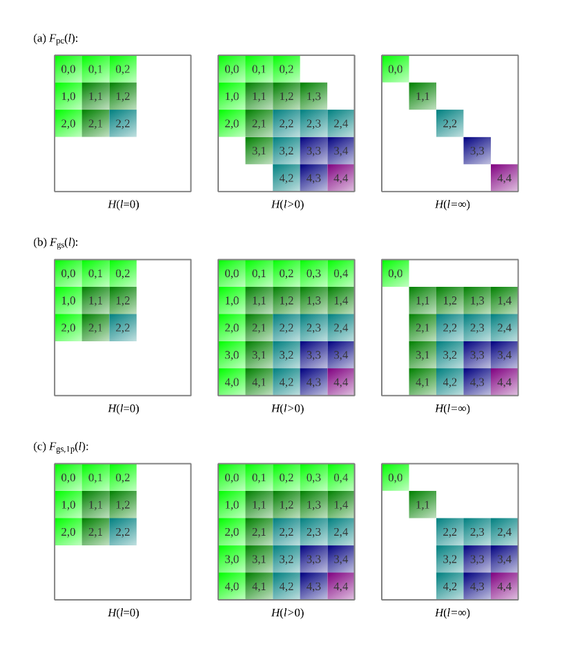
Figure 2: Schematical representation of the structure of the Hamiltonian $H(l)$ during the flow for various generators. A colored block described by the pair $i,j$ stands for the part $H^{i}_{j}(l)$ of the Hamiltonian. Only those blocks are colored where at least one term of $H^{i}_{j}(l)$ has a non-vanishing coefficient. In all cases, we assume an initial Hamiltonian which creates or annihilates at most two particles. For simplicity, we restricted our illustrations to terms which at most create or annihilate four particles for $l>0$. Of course, terms which create or annihilate more than four terms may also occur. Panel (a) shows that the generator $F_{\textrm{pc}}(l)$ conserves the block band-diagonality of the initial Hamiltonian during the flow and leads to a (quasi)particle number conserving effective Hamiltonian. Panels (b) and (c) show that both generators, $F_{\textrm{gs}}(l)$ and $F_{\textrm{gs,1p}}(l)$, do not conserve the block band-diagonality. The generator $F_{\textrm{gs}}(l)$ only separates the $H^{0}_{0}(l)$ part, whereas the generator $F_{\textrm{gs,1p}}(l)$ also decouples the $H^{1}_{1}(l)$ part.

Despite all the favorable properties of the generator $F_{\textrm{pc}}(l)$, it is not advantageous in every situation. Particularly, the last point is both a blessing and a curse. On the one hand, it ensures that the ground state is represented by the vacuum state of the effective model. Additionally, it produces the appropriate (quasi)particle picture in systems where the elementary excitations have an infinite lifetime. But on the other hand, the described ordering of the eigenstates does not reflect the situation in many physical systems, e.g. systems with unstable (quasi)particles. This is schematically illustrated in figure 1.

The generator $F_{\textrm{pc}}(l)$ interprets the energetically lowest states above the ground state as the elementary excitations. In principle, it is possible to define the elementary excitations of the system in this way. But this definition can be misleading in the sense that states with very low or zero spectral weight are regarded as the elementary excitations of the system. Without spectral weight we consider such states to be meaningless in terms of elementary excitations which serve as building blocks of all other excitations. Therefore, one usually defines the states with the largest spectral weight above the ground state as the elementary excitations of the system. Moreover, previous calculations [28, 29] strongly suggest that the rearrangement of the Hilbert space causes convergence problems in practice. In the perturbative approach of CUT [24, 30] (p-CUT) these problems become perceivable in the extrapolations [31, 32].

The second property, $\left[H_{\textrm{eff}},Q\right]=0$, of the effective Hamiltonian generated by $F_{\textrm{pc}}(l)$ makes the describtion of unstable (quasi)particles difficult. By construction, the generator $F_{\textrm{pc}}(l)$ produces an effective Hamiltonian where the elementary excitations exhibit an infinite lifetime. The information of the decay is stored in the unitary transformation and therefore an additional transformation of observables is indispensable to describe the quasiparticle decay. This approach was first used by Kehrein and Mielke to describe dissipative quantum systems [33, 34].

In the following subsection, we present a generator which does not eliminate the decay processes. Therefore, it is possible to study the quasiparticle decay more easily and more directly. The transformation of the observable is still necessary for quantitative results, but the essential aspect, i.e. the finite life time, is obvious without this transformation.

2.2 Generator for the ground state

To tackle the problems of (quasi)particle decay within the framework of CUTs mentioned in the previous section we introduce the adapted generator

$$F_{\textrm{gs}}(l)=\sum_{i>0}^{N}\left(H_{0}^{i}(l)-H_{i}^{0}(l)\right)$$ (2.6)

relying on the form of the Hamiltonian (2.2). We included only those terms in the generator $F_{\textrm{gs}}(l)$ which either contain only creation operators or contain only annihilation operators. The terms which contain only creation operators are included as they appear in $H(l)$. The terms which contain only annihilation operators are included with a negative sign relative to their sign in $H(l)$.

Again, the flow equation (2.1) converges if the spectrum is bounded from below. This follows directly from introducing a basis $\left\{\mathinner{|{i}\rangle}\right\}$, including the vacuum state $\mathinner{|{0}\rangle}$, and examining

$$\partial_{l}H_{0,0}(l)=-2\sum_{i\neq 0}\left|H_{0,i}(l)\right|^{2}$$ (2.7)

with $H_{i,j}(l):=\mathinner{\langle{i}|}H(l)\mathinner{|{j}\rangle}$. Note that $H_{i,j}(l)$ describes an explicit matrix element in contrast to the previously appearing quantity $H_{j}^{i}(l)$, which stands for a sum over terms in second quantization. According to (2.7), $H_{0,0}(l)$ is a monotonically decreasing function of $l$. Therefore, if the spectrum is bounded from below, its derivative must vanish in the limit $l\rightarrow\infty$. This also implies that

$$\lim_{l\rightarrow\infty}H_{0,i}(l)=\lim_{l\rightarrow\infty}H_{i,0}^{*}(l)=0,$$ (2.8)

i.e., all matrix elements connected to the vacuum state vanish in the limit $l\rightarrow\infty$. In contrast to the generator $F_{\textrm{pc}}(l)$ this generator destroys a block band-diagonal structure of the initial Hamiltonian $H(0)$. It solely separates the vacuum state from all other states. Hence the effective Hamiltonian is more difficult to analyze. This is the consequence of the more complex physics we have to describe. The evolution of the Hamiltonian $H(l)$ during the flow using the generator $F_{\textrm{gs}}(l)$ is compared to the one induced by $F_{\textrm{pc}}(l)$ in figure 2.

While the choice (2.6) is very plausible, we have not presented a systematic derivation of $F_{\textrm{gs}}(l)$ so far. To provide such an induction we adopt the derivation of a generator in the context of variational calculations [35]. The idea of Dawson et al. was to minimize $\partial_{l}E_{0}(l)=\partial_{l}\mathinner{\langle{0}|}H(l)\mathinner{|{0}\rangle}$ under the constraint of a bounded $F(l)$ so that the quantity $E_{0}(l)$ decreases as fast as possible. This leads to the calculation of

$$\delta\bigg{\{}\mathinner{\langle{0}|}\left[F(l),H(l)\right]\mathinner{|{0}\rangle}+\lambda\left\|F(l)\right\|^{2}_{\textrm{H}}\bigg{\}}=0$$ (2.9)

with the Lagrange multiplier $\lambda>0$ and $\left\|.\right\|_{\textrm{H}}$ denoting the Hilbert-Schmidt norm. With respect to a basis $\left\{\mathinner{|{i}\rangle}\right\}$, including $\mathinner{|{0}\rangle}$, one obtains the expression

$$\delta\Bigg{\{}\sum_{i}\bigg{(}F_{0,i}(l)H_{i,0}(l)-H_{0,i}(l)F_{i,0}(l)\bigg{)}+\lambda\sum_{i,j}\underbrace{F_{i,j}^{*}(l)}_{-F_{j,i}(l)}F_{i,j}(l)\Bigg{\}}=0$$ (2.10)

with the matrix elements $H_{i,j}(l):=\mathinner{\langle{i}|}H(l)\mathinner{|{j}\rangle}$ and $F_{i,j}(l):=\mathinner{\langle{i}|}F(l)\mathinner{|{j}\rangle}$. The variation implies

$$0=\delta_{0,i}H_{j,0}(l)-H_{0,i}(l)\delta_{j,0}-2\lambda F_{j,i}(l)$$ (2.11)

and hence

$$F_{i,j}(l)=\frac{1}{2\lambda}\left(H_{i,0}(l)\delta_{0,j}-\delta_{i,0}H_{0,j}(l)\right).$$ (2.12)

In the following, we set $\lambda={1}/{2}$ and denote this generator by $F_{\textrm{mgs}}(l)$. It has the property that only matrix elements involving the vacuum state $\mathinner{|{0}\rangle}$, i.e. $F_{i,0}(l)$ or $F_{0,i}(l)$, are different from zero. All other matrix elements vanish.

The appealing property of $F_{\textrm{mgs}}(l)$ is that there is a strong similarity to $F_{\textrm{gs}}(l)$ in the sense that the terms of $F_{\textrm{gs}}(l)$ containing only creation operators (or annihilation operators) represent the matrix elements $F_{i,0}(l)$ (or $F_{0,i}(l)$) of $F_{\textrm{mgs}}(l)$ among other processes. But the effect on the total Hilbert space is very different. The matrix $F_{\textrm{mgs}}(l)$ is active if and only if there is a direct connection to the vacuum state $\mathinner{|{0}\rangle}$, while, for instance, a term consisting only of creation operators also acts on states which already have a certain number of particles. Therefore, $F_{\textrm{gs}}(l)$ can be seen as a generalization of $F_{\textrm{mgs}}(l)$ for problems formulated in second quantization. But $F_{\textrm{gs}}(l)$ and $F_{\textrm{mgs}}(l)$ are not identical.

The question arises if it is possible to adapt the above variational derivation of the generator $F_{\textrm{mgs}}(l)$ to the generator $F_{\textrm{gs}}(l)$ formulated in second quantization. This can be achieved by modifying the applied scalar product as we show next.

We consider a system formulated in second quantization. Each operator acting on the Hilbert space can be represented by a sum over terms consisting of a product of creation and annihilation operators and a prefactor. We call the product of creation and annihilation operators a monomial. Thus a term consists of a monomial and a prefactor.

To obtain a unique representation of each monomial we first assume them to be normal ordered. Second, a certain ordering within all creation (annihilation) operators is implied. The creation and annihilation operators are denoted by $e^{{\dagger}}_{i_{k}}$ and $e^{\phantom{{\dagger}}}_{i_{k}}$, where $i_{k}$ contains all quantum numbers describing the considered operator, for instance its position and spin. Note that such an expansion of a general operator is unique since all possible (ordered) monomials are linearly independent. They can be distinguished from one another by appropriate matrix elements.

Next we define the scalar product of two monomials $M_{1}$ and $M_{2}$ by

$$\left\langle M_{1},M_{2}\right\rangle:=\cases{1&for $M_{1}=M_{2}$\\ 0&for $M_{1}\neq M_{2}$}.$$ (2.13)

Since any operator on the total Hilbert space can be expanded in monomials, (2.13) in combination with the usual bilinearity of scalar products defines a valid scalar product. The scalar product (2.13) defines different monomials as pairwise orthogonal. So the set of all possible monomials are an orthonormal basis of the super Hilbert space of operators.

The scalar product (2.13) implies the norm of an operator $O$ as $\|O\|^{2}:=\left\langle O,O\right\rangle$. We again minimize $\mathinner{\langle{0}|}\left[F(l),H(l)\right]\mathinner{|{0}\rangle}$, but with the constraint $\|F(l)\|^{2}=\textrm{const}$. Thus we calculate the variation

$$\delta\bigg{\{}\mathinner{\langle{0}|}\left[F(l),H(l)\right]\mathinner{|{0}\rangle}+\lambda\left\|F(l)\right\|^{2}\bigg{\}}=0.$$ (2.14)

The operators $H(l)$ and $F(l)$ are expanded in second quantization

$$H(l)=\sum_{\left\{\mathbf{i},\mathbf{j}\right\}}h^{\mathbf{i}}_{\mathbf{j}}(l)M^{\mathbf{i}}_{\mathbf{j}}$$ (2.15a)

and

$$F(l)=\sum_{\left\{\mathbf{i},\mathbf{j}\right\}}f^{\mathbf{i}}_{\mathbf{j}}(l)M^{\mathbf{i}}_{\mathbf{j}}$$ (2.15b)

with the $l$-dependent prefactors $\left\{h^{\mathbf{i}}_{\mathbf{j}}(l)\right\}$ and $\left\{f^{\mathbf{i}}_{\mathbf{j}}(l)\right\}$. Here the bold indices $\mathbf{i}$ and $\mathbf{j}$ are sets of indices, e.g. $\mathbf{i}=\left\{i_{1},\ldots,i_{N_{\mathbf{i}}}\right\}$. Upper indices stand for creation operators and lower indices for annihilation operators. So $M^{\mathbf{i}}_{\mathbf{j}}$ is short hand for the monomial

$$M^{\mathbf{i}}_{\mathbf{j}}=e^{{\dagger}}_{i_{1}}\cdots e^{{\dagger}}_{i_{N_{\mathbf{i}}}}e^{\phantom{{\dagger}}}_{j_{1}}\cdots e^{\phantom{{\dagger}}}_{j_{N_{\mathbf{j}}}}.$$ (2.15p)

The sums $\sum_{\left\{\mathbf{i},\mathbf{j}\right\}}$ in (2.15a) and (2.15b) run over all possible ordered sets $\mathbf{i}$ and $\mathbf{j}$ so that a unique expansion in monomials $M^{\mathbf{i}}_{\mathbf{j}}$ is achieved.

Based on (2.15a) and (2.15b) the right hand side of (2.14) to be varied has two additive contributions. The first one reads

$$\eqalign{\mathinner{\langle{0}|}\left[F(l),H(l)\right]\mathinner{|{0}\rangle}&=\mathinner{\langle{0}|}F(l)H(l)-H(l)F(l)\mathinner{|{0}\rangle}\\ &=\sum_{\left\{\mathbf{i}\right\}}\left(f_{\mathbf{i}}^{\emptyset}(l)h^{\mathbf{i}}_{\emptyset}(l)-h_{\mathbf{i}}^{\emptyset}(l)f^{\mathbf{i}}_{\emptyset}(l)\right),}$$ (2.15s)

where the empty set $\emptyset$ stands for the lack of non-trivial operators, in particular, a prefactor $f_{\mathbf{i}}^{\emptyset}(l)$ belongs to a term that only contains annihilation operators. We exploit the fact that only creation operators yield non-vanishing results if applied to $\mathinner{|{0}\rangle}$. Conversely, only annihilation operators yield non-vanishing bra states if placed right to $\mathinner{\langle{0}|}$.

The second contribution reads

$$\lambda\left(\|F(l)\|^{2}\right)=\lambda\left(\sum_{\left\{\mathbf{i},\mathbf{j}\right\}}\left|f^{\mathbf{i}}_{\mathbf{j}}(l)\right|^{2}\right).$$ (2.15t)

Making the variation with respect to $f^{\mathbf{i}}_{\mathbf{j}}(l)$ vanish leads to

$$f^{\mathbf{i}}_{\mathbf{j}}(l)=\frac{1}{2\lambda}\left(h^{\mathbf{i}}_{\emptyset}(l)\delta_{\mathbf{j},\emptyset}-\delta_{\mathbf{i},\emptyset}h_{\mathbf{j}}^{\emptyset}(l)\right).$$ (2.15u)

This generator solely contains monomials which are only composed of creation operators or only of annihilation operators. If we set $\lambda={1}/{2}$ we obtain exactly the generator $F_{\textrm{gs}}(l)$ we conjectured in (2.6). Note that the above derivation holds for all kinds of operators in second quantization, including bosons, hard-core bosons, fermions and hard-core fermions. This terminates the derivation of $F_{\textrm{gs}}(l)$ and its properties.

In this paper, we only consider the case where the generator $F_{\textrm{gs}}(l)$ separates only the vacuum state from all other states. But we want to mention that it is also possible to generalize the generator $F_{\textrm{gs}}(l)$ to the case where the vacuum state $\mathinner{|{0}\rangle}$ is replaced by a statistical operator which defines a certain subspace, i.e. a reference ensemble. In this case the generator $F_{\textrm{gs}}(l)$ induces an effective model on the reference subspace, which is separated from all other states. A well-known example is the derivation of the Heisenberg model or the $t$-$J$ model from the Hubbard model. This generalization works very much in the same way as it was done for the generator $F_{\textrm{pc}}(l)$ before [28, 29, 36, 37].

2.3 Other similar generators

Besides the two choices of a generator considered so far ($F_{\textrm{pc}}(l)$ in (2.3) and $F_{\textrm{gs}}(l)$ in (2.6)) there also exist other possibilities. For example, one can also include all terms to the generator $F_{\textrm{pc}}(l)$ which are connected to the one-particle subspace

$$F_{\textrm{gs,1p}}(l)=\sum_{i>0}^{N}\left(H_{0}^{i}(l)-H_{i}^{0}(l)\right)+\sum_{i>1}^{N}\left(H_{1}^{i}(l)-H_{i}^{1}(l)\right).$$ (2.15v)

Since this generator also separates the one-particle subspace from all subspaces with two and more particles, it is not an ideal choice to describe (quasi)particle decay. It suffers from the same caveats as $F_{\textrm{pc}}(l)$. But this generator can be the optimal choice if the (quasi)particles have an infinite lifetime, while the higher particle subspaces are overlapping in energy (cf. figure 3).

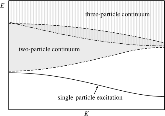
Figure 3: Overlap of the two- and three-particle continua.

In figure 2 the structure of the corresponding Hamiltonian $H(l)$ is schematically illustrated during the flow.

2.4 Common properties

Although different generators produce different CUTs and therefore lead to different effective models it happens that they transform certain subspaces in exactly the same way. For example, it can be proven (see section B.1) that all generators considered in section 2.1, section 2.2 and section 2.3 transform the vacuum state $\mathinner{|{0(l)}\rangle}$ equally. This is a consequence of the fact that for all these generators the matrix elements from and to the ground state $F_{i,0}(l)$ and $F_{0,i}(l)$, respectively, are defined in the same way as long as the flow equation is treated exactly without any truncation.

In figure 4, we show numerical data verifying the equivalent transformation of the vacuum state $\mathinner{|{0(l)}\rangle}$ by different generators.

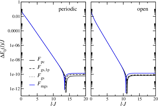
Figure 4: Evolution of $\Delta E_{0}(l):=\left|E_{0}(l)-E_{\textrm{exact}}\right|$ during the flow for an antiferromagnetic spin-${1}/{2}$ Heisenberg chain with $10$ spins and exchange coupling $J=J_{\perp}$ and $x=0$, $y=1$ (cf. (2.15aa)-(2.15ad)). All calculations started from the dimerized phase. The left panel shows the results for periodic boundary conditions; the right panel shows the results for open boundary conditions.

The $l$-dependence of the difference $\Delta E_{0}(l):=\left|E_{0}(l)-E_{\textrm{exact}}\right|$ between the vacuum expectation value $E_{0}(l):=\mathinner{\langle{0}|}H(l)\mathinner{|{0}\rangle}$ and the exact ground state energy $E_{\textrm{exact}}$ is plotted for the different generators. The system under study is an antiferromagnetic spin-${1}/{2}$ Heisenberg chain with $10$ spins and exchange coupling $J$. The starting point for all calculations is the ground state and the local triplons of the completely dimerized phase (cf. section 3). We considered periodic and open boundary conditions. Figure 4 shows clearly that all considered generators transform the vacuum state $\mathinner{|{0(l)}\rangle}$ in the same way. The features beyond $l\approx 12/J_{\perp}$ stem from numerical inaccuracies occurring at $\Delta E\approx 10^{-10}J$. These inaccuracies are shown here to illustrate where and how numerical errors make themselves felt.

Similarly, one can prove that the generator $F_{\textrm{pc}}(l)$ and the generator $F_{\textrm{gs,1p}}$ transform all one-particle states identically (see section B.2).

3 Model: Asymmetric antiferromagnetic spin-${1}/{2}$ Heisenberg ladder

The Hamiltonian for the asymmetric antiferromagnetic ($J_{\parallel},J_{\perp},J_{\textrm{diag}}>0$) spin-${1}/{2}$ Heisenberg ladder reads

$$H=J_{\perp}\left(H_{\perp}+xH_{\parallel}+yH_{\textrm{diag}}\right)$$ (2.15aa)

with

$$H_{\perp} = \sum_{r}\boldsymbol{S}_{1,r}\boldsymbol{S}_{2,r}$$ (2.15ab)

$$H_{\parallel} = \sum_{r}\left(\boldsymbol{S}_{1,r}\boldsymbol{S}_{1,r+1}+\boldsymbol{S}_{2,r}\boldsymbol{S}_{2,r+1}\right)$$ (2.15ac)

$$H_{\textrm{diag}} = \sum_{r}\boldsymbol{S}_{1,r}\boldsymbol{S}_{2,r+1},$$ (2.15ad)

where the first subscript $1,2$ denotes the leg and $r$ the rung (see figure 6). The parameter $x$ is given by $x:={J_{\parallel}}/{J_{\perp}}$ and the parameter $y$ by $y:={J_{\textrm{diag}}}/{J_{\perp}}$.

This Hamiltonian contains some frequently discussed models. For example, for $x=0$ and $y=1$ the Hamiltonian (2.15aa)-(2.15ad) describes the exactly solvable isotropic antiferromagnetic spin-${1}/{2}$ Heisenberg chain [38, 39, 40, 41, 42, 43, 44]. In the broad field of spin systems without magnetic long-range order the limit of the symmetric spin-${1}/{2}$ Heisenberg ladder [45, 46, 47, 48, 49, 50, 51, 52, 53, 54, 55, 56, 31] (see figure 5) with $y=0$ is very popular as one-dimensional example of a valence-bond solid. Besides the theoretical interest in $H$ in (2.15aa)-(2.15ad), there is a large number of compounds which can be described by spin ladders (see e.g. [57, 58, 59, 60, 61, 62, 63, 64, 65, 66] or for an overview [67]). Special interest has been raised by the realization of coupled spin ladders in the stripe phases of cuprate superconducters [68, 69, 70]. Also the experimental evidence for superconductivity in Sr_0.4Ca_13.6Cu₂₄O₄₁ under pressure [71] contributed to the interest in the spin-${1}/{2}$ Heisenberg ladder and its extended versions. For the case $x<y$ the Hamiltonian (2.15aa)-(2.15ad) is usually denoted as dimerized and frustrated spin-${1}/{2}$ Heisenberg chain (see [72] and references therein).

In the following, we study the two parameter sets $x=0.5$, $y=0$ and $x=0.5$, $y=0.1$ in the thermodynamic limit as generic examples. Since in both cases the relation $x>y$ is fulfilled we call the system an asymmetric ladder instead of a dimerized and frustrated chain. A more comprehensive investigation of the dependences of the quasiparticle decay on the model parameter is left to ongoing research. The scope of this section and the next one is to illustrate the general considerations concerning the method by a concrete example.

The low energy spectrum for $x=0.5$ and $y=0$ is well studied by several methods (see e.g. [47] and [51]) including methods based on CUTs [73]. Therefore, it is a perfect starting point to discuss the more sophisticated case with $x=0.5$ and $y=0.1$. The additional diagonal interaction $y$ makes the whole situation conceptionally more difficult because it breaks a symmetry. While for $y=0$ the model is symmetric under reflection (see figure 5) an arbitrary small value $y\neq 0$ breaks this reflection symmetry (see figure 6).

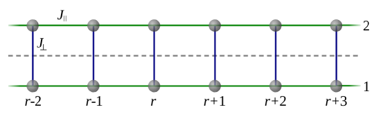
Figure 5: Schematic representation of a spin ladder. Circles indicate spins with $S={1}/{2}$. Solid lines stand for couplings. The dashed line indicates the axis of reflection symmetry.

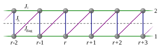
Figure 6: Schematic representation of the asymmetric spin ladder. The additional diagonal interaction $J_{\textrm{diag}}$ breaks the reflection symmetry and hence induces a hybridization between the one-quasiparticle states and the two-quasiparticle continuum. Thus it is an ideal model to study quasiparticle breakdown.

The crucial point is that the reflection symmetry of the symmetric ladder is responsible for the infinite lifetime of the triplons, which are the $S=1$ elementary magnetic excitations of an antiferromagnetic system without long-range order [74]. Breaking this symmetry creates processes which enable the triplons to decay into two-triplon states. Therefore, the asymmetric spin-${1}/{2}$ Heisenberg ladder is an ideal model to analyze quasiparticles with finite lifetime and to illustrate our previous theoretical considerations concerning the choice of an adaptive generator quantitatively.

To define an appropriate starting point for the CUTs we use the bond operator representation [75, 76]. Each rung $r$ of the ladder considered separately has a four dimensional Hilbert space. A possible eigenbasis of the local operator $\boldsymbol{S}_{1,r}\boldsymbol{S}_{2,r}$ is given by the singlet state

$$\mathinner{|{s}\rangle}_{r}:=\frac{1}{\sqrt{2}}\left(\mathinner{|{\uparrow\downarrow}\rangle}-\mathinner{|{\downarrow\uparrow}\rangle}\right)_{r}$$ (2.15aba)

and the three triplet states

$$t_{x,r}^{{\dagger}}\mathinner{|{s}\rangle}_{r}:=\mathinner{|{t_{x}}\rangle}_{r}= \frac{-1}{\sqrt{2}}\left(\mathinner{|{\uparrow\uparrow}\rangle}-\mathinner{|{\downarrow\downarrow}\rangle}\right)_{r}$$ (2.15abb)

$$t_{y,r}^{{\dagger}}\mathinner{|{s}\rangle}_{r}:=\mathinner{|{t_{y}}\rangle}_{r}= \frac{\rmi}{\sqrt{2}}\left(\mathinner{|{\uparrow\uparrow}\rangle}+\mathinner{|{\downarrow\downarrow}\rangle}\right)_{r}$$ (2.15abc)

$$t_{z,r}^{{\dagger}}\mathinner{|{s}\rangle}_{r}:=\mathinner{|{t_{z}}\rangle}_{r}= \frac{1}{\sqrt{2}}\left(\mathinner{|{\uparrow\downarrow}\rangle}+\mathinner{|{\downarrow\uparrow}\rangle}\right)_{r}.$$ (2.15abd)

Without any interactions along the ladder ($x=0$, $y=0$) the ground state of the system is the product state of the rung singlets

$$\mathinner{|{0}\rangle}:=\prod_{r}\mathinner{|{s}\rangle}_{r}.$$ (2.15abc)

This reference state shall be the vacuum state of the system. Excitations on a rung $r$ are created by the local operators $t_{x,r}^{{\dagger}}$, $t_{y,r}^{{\dagger}}$ and $t_{z,r}^{{\dagger}}$. These operators create a triplet on the rung $r$ and satisfy the hard-core boson commutation relations

$$\left[t_{\alpha,r}^{\phantom{{\dagger}}},t_{\beta,s}^{{\dagger}}\right]=\delta_{r,s}\left(\delta_{\alpha,\beta}-t_{\beta,r}^{{\dagger}}t_{\alpha,r}^{\phantom{{\dagger}}}-\delta_{\alpha,\beta}\sum_{\gamma}\left(t_{\gamma,r}^{{\dagger}}t_{\gamma,r}^{\phantom{{\dagger}}}\right)\right),$$ (2.15abd)

where $t_{\alpha,r}$ ($\alpha=x,y,z$) annihilate such a triplet. We consider all the excited states, which can be continuously connected to the local triplets, to be the elementary magnetic excitations. They are called triplons [74, 31].

In the bond operator representation the Hamiltonian (2.15aa)-(2.15ad) is given in the notation of (2.2) by

$$H=J_{\perp}\left(H_{0}^{0}+H_{1}^{1}+H_{2}^{2}+H_{0}^{2}+H_{2}^{0}+H_{1}^{2}+H_{2}^{1}\right)$$ (2.15abea)

with

$$H_{0}^{0}=-\sum_{r}\frac{3}{4}$$ (2.15abeb)

$$\eqalign{H_{1}^{1}=\sum_{r}t^{{\dagger}}_{\alpha,r}t^{\phantom{{\dagger}}}_{\alpha,r}+\left(\frac{1}{2}x-\frac{1}{4}y\right)\sum_{r}\sum_{\alpha}\left(t^{{\dagger}}_{\alpha,r}t^{\phantom{{\dagger}}}_{\alpha,r+1}+t^{{{\dagger}}}_{\alpha,r+1}t^{\phantom{{\dagger}}}_{\alpha,r}\right)}$$ (2.15abed)

$$\eqalign{H_{2}^{2}=\left(\frac{1}{2}x+\frac{1}{4}y\right)\sum_{r}\sum_{\alpha\neq\beta}t^{{\dagger}}_{\alpha,r}t^{{{\dagger}}}_{\beta,r+1}t^{\phantom{{\dagger}}}_{\beta,r}t^{\phantom{{\dagger}}}_{\alpha,r+1}\\ -\left(\frac{1}{2}x+\frac{1}{4}y\right)\sum_{r}\sum_{\alpha\neq\beta}t^{{\dagger}}_{\alpha,r}t^{{{\dagger}}}_{\alpha,r+1}t^{\phantom{{\dagger}}}_{\beta,r}t^{\phantom{{\dagger}}}_{\beta,r+1}}$$ (2.15abeg)

$$H_{0}^{2}=\left(\frac{1}{2}x-\frac{1}{4}y\right)\sum_{r}\sum_{\alpha}t^{{\dagger}}_{\alpha,r}t^{{{\dagger}}}_{\alpha,r+1}$$ (2.15abeh)

$$H_{2}^{0}=\left(H_{0}^{2}\right)^{{\dagger}}$$ (2.15abei)

$$H_{1}^{2}=-\frac{\rmi}{4}y\sum_{r}\sum_{\alpha,\beta,\gamma}\varepsilon_{\alpha\beta\gamma}\left(t^{{\dagger}}_{\alpha,r}t^{{{\dagger}}}_{\beta,r+1}\left(t^{\phantom{{\dagger}}}_{\gamma,r}+t^{\phantom{{\dagger}}}_{\gamma,r+1}\right)\right)$$ (2.15abej)

$$H_{2}^{1}=\left(H_{1}^{2}\right)^{{\dagger}}.$$ (2.15abek)

This representation of the Hamiltonian of the asymmetric antiferromagnetic spin-${1}/{2}$ Heisenberg ladder is used as the starting point for the CUTs. For $y=0$ the terms (2.15abej) and (2.15abek) vanish whereby decay processes of one triplon into two are prevented.

Evaluating the commutator $\left[F(l),H(l)\right]$ appearing on the right hand side of the flow equation (2.1) generates also terms which do not appear in the initial Hamiltonian $H(0)=H$. These terms must be added to the Hamiltonian with a coefficient equal to zero at $l=0$. They must also be considered in the generator. Then the commutator $\left[F(l),H(l)\right]$ generates even more terms which have to be taken into account. For a finite-dimensional Hilbert space this procedure comes to an end because the maximal number of terms is restricted. Such unrestricted calculations were performed to compute the results for the ground-state energy of the finite Heisenberg chain presented in section 2.4.

For large systems such an unrestricted approach is not possible due to the proliferating number of terms. Especially in the thermodynamic limit, one has to deal with an infinite number of terms. Hence it is not possible to obtain a closed set of differential equations. Thus in practice one has to decide which terms are important to describe the underlying physics properly and which terms can be neglected.

One established truncation scheme is to use a perturbative approach [24, 30] (p-CUT) which is based on the generator $F_{\textrm{pc}}(l)$. But since we intend to describe the decay of quasiparticles so that variations of the generator $F_{\textrm{pc}}(l)$ (see section 2) have to be used, we choose the self-similar approach (s-CUT). But there is no fundamental reason why the adapted generator cannot be implemented perturbatively as well.

The s-CUT was used in many previous applications of the CUTs (for an overview see [77] and references therein) among them the original work by Wegner [15]. The whole transformation takes place in the coefficients of the terms in the Hamiltonian which motivates the naming “self-similar”. This approach can straightforwardly be implemented for various generators.

In the present paper, we apply the following truncation scheme, which is based on the finite correlation length of one-dimensional systems with a finite gap. The truncation scheme is based on the locality of the term which is justified for systems with finite correlation length. It is described in detail in the following section 3.1.

All in all we proceed in the actual calculations as follows:

• Define a truncation scheme which restricts the maximal number of terms.

• Set up the flow equation by calculating the commutator $\left[F(l),H(l)\right]$. Only those terms are considered which fit the truncation scheme.

• Solve the flow equation numerically.

For calculations in the thermodynamic limit, it is necessary to make use of the translational invariance of the Hamiltonian (2.15abea)-(2.15abek). The translation symmetry ensures that terms which describe identical processes except for a shift along the ladder have the same coefficient. Consequently, it is sufficient to track only one representative of this symmetry group. This procedure is also possible for all others symmetries of the Hamiltonian (2.15abea)-(2.15abek), e.g., the spin symmetry and the rotational symmetry by $\pi$ of the ladder. Using representatives of the underlying symmetries reduces the number of coefficients appearing in the flow equation (2.1) significantly for a given truncation scheme. Thus more extended truncation schemes considering more processes become feasible.

3.1 Truncation scheme

A truncation scheme is necessary to limit the number of terms so that a closed set of differential equations is achieved. In the present paper, we are dealing with terms in real-space and the truncation scheme is based on the locality of the terms. We first define a measure for the locality of a term, which we call the extension $d$. The extension $d$ of a term is defined by the distance between the rightmost to the leftmost rung on which the monomial acts in a nontrivial way. For example, the term $t^{{\dagger}}_{\alpha,r}t^{{{\dagger}}}_{\beta,r+1}t^{\phantom{{\dagger}}}_{\gamma,r+4}$ has an extension $d=4$. Second, we define the truncation scheme by choosing a maximal extension $d_{\textrm{max}}$ discarding all terms with a larger extension ($d>d_{\textrm{max}}$).

It turns out that it is appropriate to define not only one maximal extension for all terms but to keep terms with a different number of annihilation or creation operators up to different maximal extensions [29]. Accordingly, terms with $n$ annihilation or creation operators in total are required to have an extension $d_{n}$ or less to be kept in the flow equation. As a second truncation criterion we admit only terms which create or annihilate not more than $N$ (quasi)particles. Thus the total truncation scheme is defined by the value of $N$ and the set of extensions $\mathbf{d}=\left(d_{2},\ldots,d_{2N}\right)$. Note that due to the conservation of spin no single triplon operators can occur in the Hamiltonian. So no $d_{1}$ needs to be denoted. In addition, the translational invariance of the Hamiltonian makes $d_{1}$ superfluous. In this case only six different monomials exist which act on one rung only, in particular, $t^{{\dagger}}_{\alpha,r}$ and $t^{\phantom{{\dagger}}}_{\alpha,r}$ with $\alpha=x,y,z$. For the symmetric ladder ($y=0$) no terms occur which consist of an odd number of operators. Therefore, we do not need to define maximum extensions $d_{3},d_{5},\ldots$ . In the notation of the set of extensions $\mathbf{d}$ we replace such superfluous extensions by a dot, e.g. $\mathbf{d}=(8,.,6,.,4)$.

It is worthwhile to emphasize that this truncation scheme does not turn our approach to a calculation on a finite cluster. It is a self-similar calculation strictly in the thermodynamic limit. We only truncate the range of the interactions in real space, but not the Hilbert space.

4 Results

Here we present results for the symmetric ladder with $x=0.5$ and $y=0$ and for the asymmetric ladder with $x=0.5$ and $y=0.1$. These two parameter sets are chosen to illustrate the differences between systems with stable quasiparticles and systems with unstable quasiparticles which exhibit a finite lifetime. In particular, we confirm our previous statements concerning the properties of the different generators (cf. section 2).

Firstly we show that a rearrangement of the states of the Hilbert space, i.e., a continuous re-labelling (for simple examples see [21]), reduces the speed of convergence (see section 4.1). Therefore, generators which avoid such a rearrangement induce a considerably faster convergence. Secondly, we discuss the low energy spectrum for the symmetric and for the asymmetric ladder (see section 4.2). If decay is possible the generator $F_{\textrm{gs,1p}}(l)$ and the generator $F_{\textrm{pc}}(l)$ indeed tend to interpret the energetically lowest states above the ground state as the elementary excitations (as stated before in section 2). This can be avoided by using the generator $F_{\textrm{gs}}(l)$. Unfortunately, for this generator a simple calculation in the one-particle subspace is not sufficient to arrive at reliable results for the true one-triplon dispersion. This is a consequence of the fact that in the effective Hamiltonian induced by $F_{\textrm{gs}}(l)$ the one-particle subspace still couples to higher particle subspaces (see figure 2). To obtain reliable results for the single triplon dispersion we include states which consist of up to three particles in our calculations (see section 4.3). Especially, we show results for the zero temperature spectral density in which the (quasi)particle decay is manifest as a Lorentzian resonance of finite width.

4.1 Convergence

To quantify the speed of convergence of the flow equation for different generators we introduce the residual off-diagonality (ROD) [28, 29]. The ROD is defined as the square root of the sum of the moduli squared of all coefficients that contribute to the considered generator. Using the notation of (2.15b) the ROD is given by

$$\textrm{ROD}(l)=\sqrt{\sum_{\left\{\mathbf{i},\mathbf{j}\right\}}\left|f^{\mathbf{i}}_{\mathbf{j}}(l)\right|^{2}}$$ (2.15abea)

where the range of the sum $\sum_{\left\{\mathbf{i},\mathbf{j}\right\}}$ depends on the choice of the generator. Note that only one representative of the translational symmetry group is included. Otherwise the ROD would grow proportional to the system size. In addition, ROD${}^{i}_{j}$ denotes the square root of the sum of the moduli squared of all coefficients belonging to terms with $i$ creation and $j$ annihilation operators or to their Hermitian conjugate terms.

Figure 7a shows the evolution of the ROD during the flow for different generators and different truncation schemes for $x=0.5$ and $y=0$.

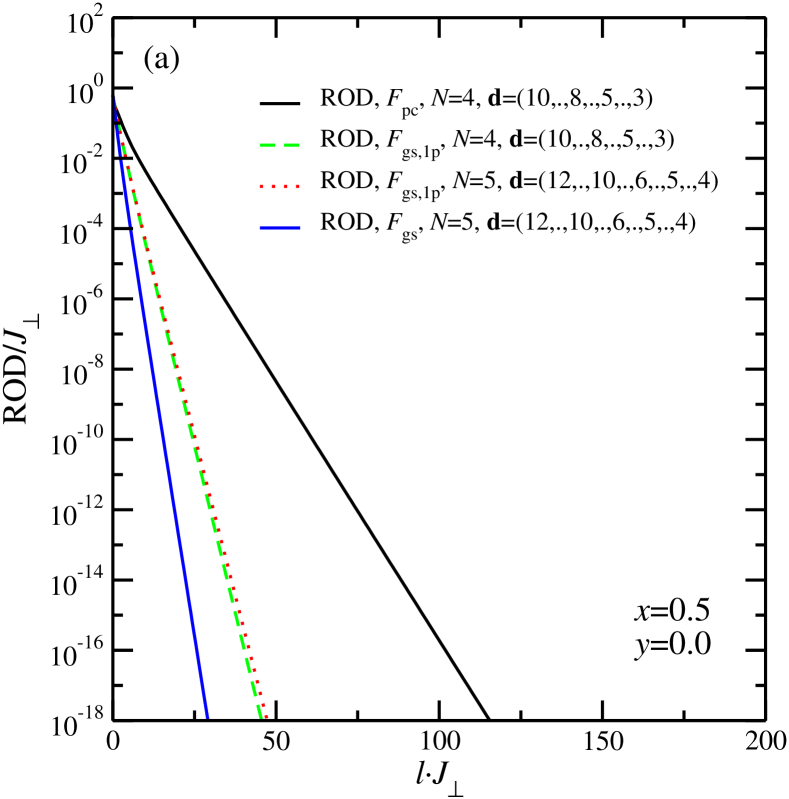
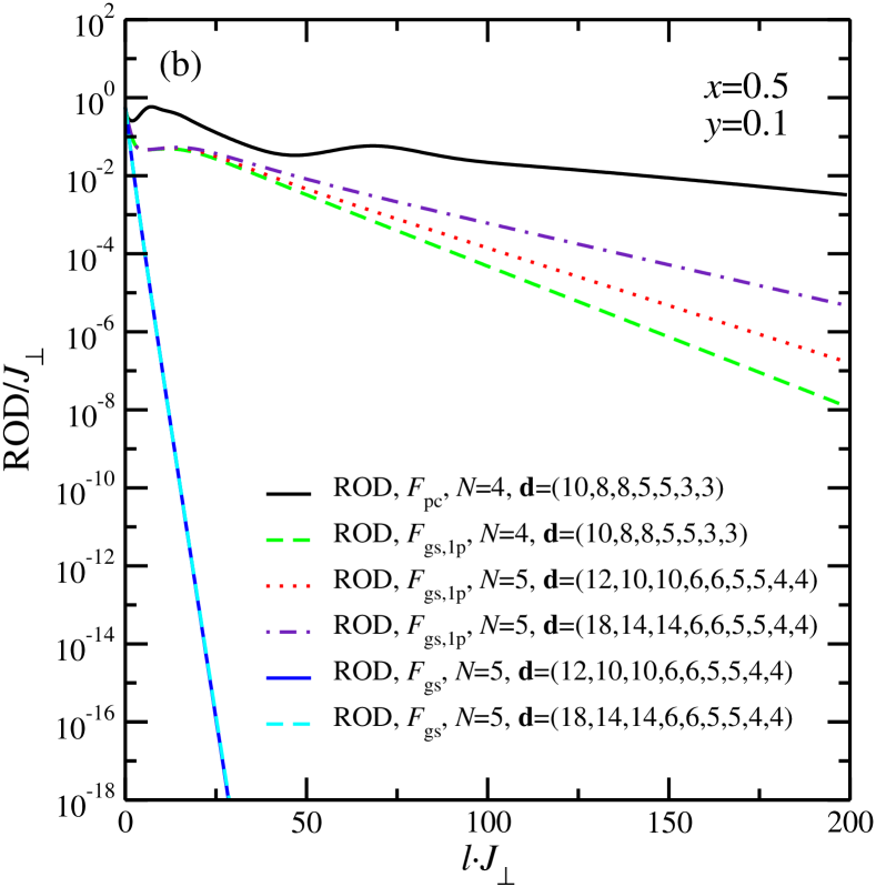
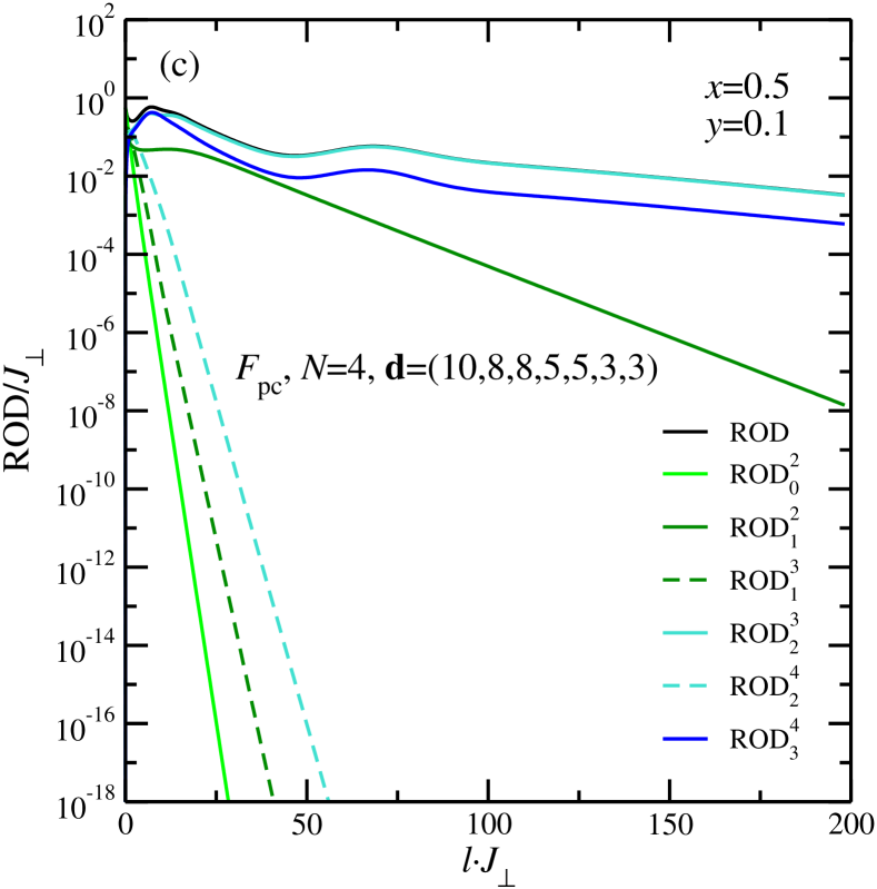
Figure 7: Convergence of the flow equations. Panel (a) shows the evolution of the ROD during the flow for different generators and different truncation schemes for the symmetric ladder ($x=0.5$ and $y=0$). In all cases the ROD decreases strictly monotonically. Panel (b) shows the evolution of the ROD for different generators and different truncation schemes for the asymmetric ladder ($x=0.5$ and $y=0.1$). The RODs of the generator $F_{\textrm{gs,1p}}(l)$ and the generator $F_{\textrm{pc}}(l)$ increase temporarily during the flow. This indicates a significant rearrangement of the states in the Hilbert space. Panel (c) shows the ROD of the generator $F_{\textrm{pc}}(l)$ split in the parts ROD${}^{i}_{j}$ for the asymmetric ladder ($x=0.5$ and $y=0.1$). The main contributions to the total ROD is due to ROD${}^{i}_{j}$ with $|i-j|=1$.

For all generators the RODs decrease strictly monotonically. The ROD of the generator $F_{\textrm{gs}}(l)$ decreases faster than the ROD of the generator $F_{\textrm{gs,1p}}(l)$. This is a consequence of the fact that the generator $F_{\textrm{gs,1p}}(l)$ contains more coefficients than the generator $F_{\textrm{gs}}(l)$. The convergence of these additional coefficients is slower because they connect states which differ less in their eigenenergies (cf. (2.15abeeimj)), e.g. the energy gap between one- and three-triplon states is smaller than the energy gap between the vacuum state and the two-triplon states. This also explains why the generator $F_{\textrm{gs,1p}}(l)$ converges faster than the generator $F_{\textrm{pc}}(l)$.

The convergence behavior clearly changes if one includes the diagonal interaction, even if $y$ is small ($y=0.1$). In figure 7b the ROD during the flow for different generators and different truncation schemes for $x=0.5$ and $y=0.1$ is depicted. Only the ROD of the generator $F_{\textrm{gs}}(l)$ decreases strictly monotonically while the RODs of the generator $F_{\textrm{gs,1p}}(l)$ and the generator $F_{\textrm{pc}}(l)$ increase temporarily during the flow. These increases indicate a rearrangement in the Hilbert space, cf. [21] for simple examples. If all eigenstates were ordered in such a way that states with more triplons had higher eigenenergies the ROD would decrease exponentially (cf. (2.15abeeimg)). These rearrangements affect the results for the one-triplon dispersion as we illustrate in the section 4.2.

Figure 7c shows the ROD of the generator $F_{\textrm{pc}}(l)$ split in the partial RODs ROD${}^{i}_{j}$ defined above for $x=0.5$ and $y=0.1$. Clearly, the contributions ROD${}^{i}_{j}$ of the ROD changing the number of triplons only by one ($|i-j|=1$) provide the main contributions to the total ROD, although the corresponding initial couplings are proportional to $y$, which is small ($y=0.1$). From this we infer that the convergence of the flow equation is mainly influenced by terms which induce a rearrangement of the Hilbert space if they are to be eliminated by the CUT. It is less important whether the corresponding coupling parameter is large or not. This is an important property of the CUTs which distinguishes them from conventional diagrammatic perturbation theories.

In summary, we state that a rearrangement of the states of the Hilbert space reduces the speed of convergence. Omitting the corresponding terms from the generator stabilizes the flow in the sense that the convergence is monotonic and robust. Hence, especially the generator $F_{\textrm{gs}}(l)$ yields a very fast converging and robust flow. We point out that a fast convergence is advantageous because it minimizes the interval in $l$ during which significant terms are truncated. Hence as a rule of thumb, the faster the convergence, the smaller are the truncation errors.

4.2 Low energy spectrum

Here we discuss the low energy spectrum of the effective Hamiltonian $H_{\textrm{eff}}$. We always stopped the CUT at $l=200/J_{\perp}$. At this value the remaining effect on the one-particle subspace is small in all cases (cf. figure 7) so that a further integration of the flow equation would not change the results for the one-triplon dispersion as shown in figure 8.

To calculate the one-triplon dispersion $\omega_{1}(K)$ of the effective model we define the Fourier-transformed one-particle states

$$\mathinner{|{K,\alpha}\rangle}:=\frac{1}{\sqrt{\mathcal{N}}}\sum_{r}\rme^{\rmi Kr}\mathinner{|{r,\alpha}\rangle}$$ (2.15abeb)

with $\mathinner{|{r,\alpha}\rangle}:=t^{{\dagger}}_{\alpha,r}\mathinner{|{0}\rangle}$. The action of $H_{1}^{1}(l)$ with respect to the translational symmetry is given by (D.1) in section D. Due to the SU(2) symmetry of the Hamiltonian $H(l)$ the hopping coefficients $c_{11;{r}}^{\alpha^{\prime},\alpha}$ obey the relation $c_{11;{r}}^{\alpha^{\prime},\alpha}=\delta_{\alpha^{\prime},\alpha}c_{11;r}$. This leads to the threefold degenerate one-triplon dispersion

$$\omega_{1}(K):=\mathinner{\langle{K,\alpha}|}H_{1}^{1}(\infty)\mathinner{|{K,\alpha}\rangle}=\sum_{{r}}\rme^{\rmi K{r}}c_{11;{r}}\ .$$ (2.15abec)

The generator $F_{\textrm{pc}}(l)$ and the generator $F_{\textrm{gs,1p}}(l)$ separate the one-particle subspace from the other subspaces. Consequently, for these two generators the one-triplon dispersion $\omega_{1}(K)$ yields eigenvalues of the effective Hamiltonian $H_{\textrm{eff}}$ in the one-particle subspace. In contrast, the generator $F_{\textrm{gs}}(l)$ does not separate the one-particle space. Therefore, the effective Hamiltonian $H_{\textrm{eff}}$ still contains terms which connect the one-particle subspace with higher particle states. In this case the quantity $\omega_{1}(K)$ only gives an approximation of the eigenvalues of the effective Hamiltonian $H_{\textrm{eff}}$ (cf. figure 12a).

In figure 8a the one-triplon dispersion $\omega_{1}(K)$ is displayed for $x=0.5$ and $y=0$.

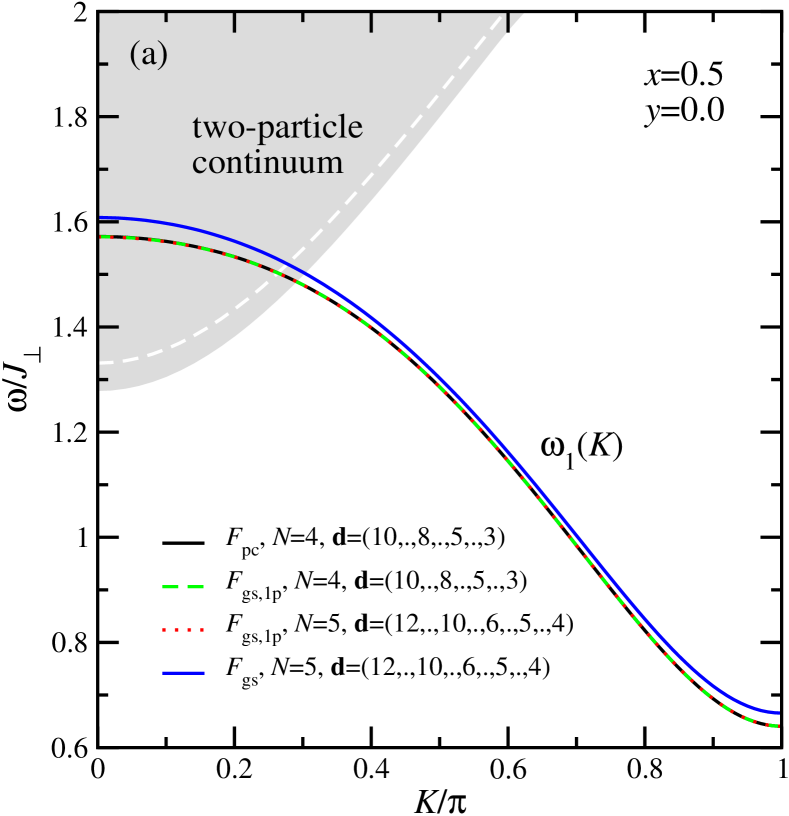
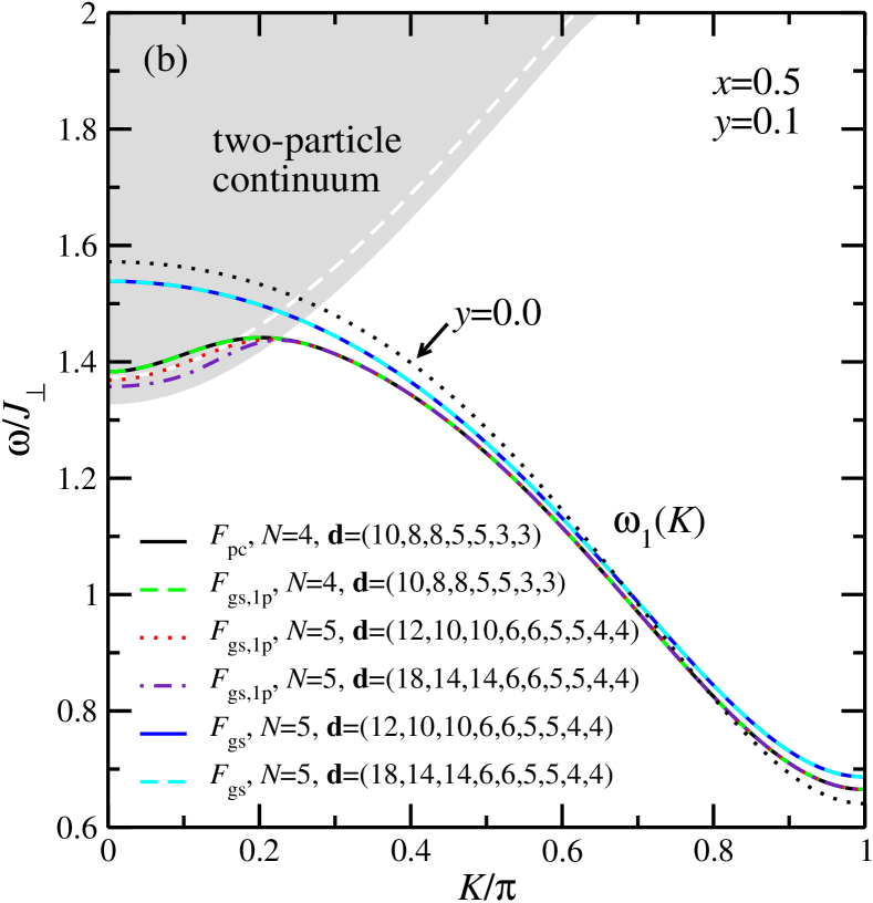
Figure 8: Low energy spectrum of the symmetric and asymmetric spin-${1}/{2}$ Heisenberg ladder. Panel (a) shows results for the one-triplon dispersion $\omega_{1}(K)$ for the symmetric ladder with $x=0.5$ and $y=0$. Results for different generators and different truncation schemes are depicted. Additionally, the lower part of the two-particle continuum is shown (grey area). The dashed white line represents an approximation of the lower edge of the two-particle continuum obtained by the approximate one-triplon dispersion $\omega_{1}(K)$ in the case of the generator $F_{\textrm{gs}}(l)$. Panel (b) shows the corresponding quantities for the asymmetric ladder with $x=0.5$ and $y=0.1$.

Results for all three generators $F_{\textrm{pc}}(l)$, $F_{\textrm{gs,1p}}(l)$ and $F_{\textrm{gs}}(l)$ and various truncation schemes are shown. The two generators $F_{\textrm{pc}}(l)$ and $F_{\textrm{gs,1p}}(l)$ separating the one-particle space yield almost the same results and barely depend on the chosen truncation scheme. Together with the good convergence (cf. figure 7a) this implies that the results are very reliable. By construction, for the generator $F_{\textrm{gs}}(l)$ the quantity $\omega_{1}(K)$ as defined above yields only an approximation of the true one-triplon dispersion. The resulting $\omega_{1}(K)$ is an upper bound to the results obtained from the other two generators if the truncation errors are negligible. This fact is based on the variational principle that a minimum in a restricted subspace is an upper bound to the minimum in an unrestricted subspace. To improve the results in this case one has to consider higher particle subspaces as well (cf. section 4.3).

Figure 8 also displays the lower part of the two-particle continuum

$$\omega_{2}(K,Q)=\omega_{1}\left({K}/{2}+Q\right)+\omega_{1}\left({K}/{2}-Q\right),$$ (2.15abed)

where $Q\in\left[-\pi,\pi\right]$ denotes the relative momentum. The lower band edge is given by the minimum of $\omega_{2}(K,Q)$ over $Q$; the maximum yields the upper band edge, respectively. Here we used the one-triplon dispersion $\omega_{1}(K)$ we obtained by the generator $F_{\textrm{pc}}(l)$. The additional dashed white line represents an approximation of the lower edge of the two-particle continuum obtained by the approximate one-triplon dispersion $\omega_{1}(K)$ in the case of the generator $F_{\textrm{gs}}(l)$. We emphasize again that due to the reflection symmetry for $y=0$ (cf. figure 5) no interaction exists between the one-triplon states and the two-particle continuum. As a result the quasiparticles are well-defined and infinitely long-lived for the whole Brillouin zone, although the two-particle continuum starts below the one-triplon dispersion for certain momenta $K$. In addition, this symmetry prevents any rearrangement between the one- and two-particle subspaces during the flow (see section A). This situation changes abruptly if a diagonal interaction is switched on, even if $y$ is very small.

In figure 8b the one-triplon dispersion $\omega_{1}(K)$ is displayed for $x=0.5$ and a small additional diagonal interaction $y=0.1$. Again results for all three generators $F_{\textrm{pc}}(l)$, $F_{\textrm{gs,1p}}(l)$ and $F_{\textrm{gs}}(l)$ and various truncation schemes are shown as well as the lower part of the two-particle continuum $\omega_{2}(K,Q)$ determined from the one-triplon dispersion obtained by the generator $F_{\textrm{pc}}(l)$. Likewise, the approximate results for the lower edge of the two-particle continuum obtained by the generator $F_{\textrm{gs}}(l)$ are shown. For comparison only, we also included the former results of the one-triplon dispersion obtained by the generator $F_{\textrm{pc}}(l)$ for $x=0.5$ and $y=0$.

The use of the two generators $F_{\textrm{pc}}(l)$ and $F_{\textrm{gs,1p}}(l)$ implies significantly lower energies for the one-triplon dispersion, see figure 8b, where $\omega_{1}(K)$ overlaps with the two-triplon continuum. The results strongly depend on the truncation scheme in this region. This can be explained as follows. Since for $y\neq 0$ the one-particle and the two-particle space are interacting with each other, the two generators $F_{\textrm{pc}}(l)$ and $F_{\textrm{gs,1p}}(l)$ try to sort the eigenvalues in such a way that the eigenvalues of the one-triplon dispersion lie below the two-particle continuum, see figure 1 and section A. Therefore, the one-triplon dispersion of the effective model $H_{\textrm{eff}}$ lies at the lower edge of the two-particle continuum in the region where the one-triplon dispersion merges with the two-particle continuum. This is not completely achieved in practice because of the indispensable usage of a truncation scheme.

We truncate the range of the decay processes in real space. This means that the distance between the generated two triplons is limited although the true scattering state comprises contributions up to infinite distances. As a result, the rearrangement of the eigenvalues is only incomplete. Figure 8b illustrates that increasing the range of the decay processes (e.g. increasing $d_{3}$) implies that $\omega_{1}(K)$ approaches the lower band edge of $\omega_{1}(K,Q)$ from above more and more.

As stated before, the rearrangements of the states are unfavorable for two reasons. (i) They imply a slow convergence which may cause growing truncation errors. (ii) One usually defines the state with the largest spectral weight above the ground state as the elementary excitation of the system and not a state with almost no spectral weight, even if it is lower in energy.

To avoid the rearrangement of the eigenstates, which leads to a potentially misleading quasiparticle picture, we employ the operator $F_{\textrm{gs}}(l)$ (cf. figure 8b). As before the generator $F_{\textrm{gs}}(l)$ only yields an approximation for the one-triplon eigenvalues of the effective Hamiltonian $H_{\textrm{eff}}$. This is the case even in the region of the Brillouin zone where the quasiparticles are well-defined. Due to our treatment of the problem in real space we cannot distinguish processes in different regions in momentum space easily. To improve the results for the one-triplon dispersion one must consider the interaction with states which consists of more than one particle as well. This is discussed in the next section 4.3.

Here, we first want to show the results for the two- and three-particle continua resulting from the approximate one-triplon dispersion $\omega_{1}(K)$ in the case of the generator $F_{\textrm{gs}}(l)$ for $x=0.5$ and $y=0.1$. The three-particle continuum can be determined in analogy to the two-particle continuum. One only has to replace one one-triplon dispersion on the right hand side of (2.15abed) by energies of the two-particle continuum.

The boundaries of these continua are shown in figure 9 by solid lines.

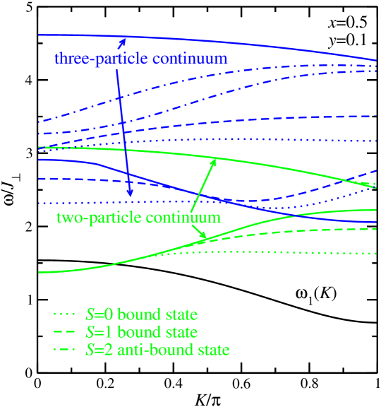
Figure 9: Two- and three-triplon continua of the asymmetric spin-${1}/{2}$ Heisenberg ladder with $x=0.5$ and $y=0.1$. The solid green lines represent the lower and upper boundaries of the two-particle continuum. The other green lines represent two two-particle bound states and one two-particle anti-bound state. The blue lines illustrate the boundaries of the three-particle continuum, where the type of the lines correspond to the two-particle state(s) used to determine the three-particle continuum.

Additionally, this figure shows the boundaries of the three-particle continua emerging from the combination of the approximate one-triplon dispersion $\omega_{1}(K)$ and a certain approximate two-particle (anti-)bound state. Here we only use the region where the corresponding (anti-)bound state is well-defined, i.e., does not merge with the continuum.

The two-particle bound states and the two-particle anti-bound state shown in figure 9 are calculated by diagonalizing the effective Hamiltonian $H_{\textrm{eff}}$ in the subspace spanned by the single-triplon states

$$\mathinner{|{K,\alpha}\rangle}:=\frac{1}{\sqrt{\mathcal{N}}}\sum_{r}\rme^{\rmi Kr}\mathinner{|{r,\alpha}\rangle}$$ (2.15abeea)

and the two-triplon states

$$\mathinner{|{K,\alpha}\rangle}\mathinner{|{d,\beta}\rangle}:=\frac{1}{\sqrt{\mathcal{N}}}\sum_{r}\rme^{\rmi K\left(r+\frac{d}{2}\right)}\mathinner{|{r,\alpha}\rangle}\mathinner{|{r+d,\beta}\rangle}$$ (2.15abeeb)

with $0<d<120$ for each given value of $K$ (for details see section D).

Since the subspace spanned by the states (2.15abeea) and (2.15abeeb) is not separated from higher triplon states (cf. figure 12b we obtain – as for the one-triplon dispersion $\omega_{1}(K)$ – only an approximation for the bound states. Consequently, the depicted continua only represent approximations as well. The restriction of the relative distance $d$ in the two-triplon subspace (2.15abeeb) is less important. Increasing $d$ does not change the results perceivably.

As in the symmetric case $x=0.5$ and $y=0$ [78, 79, 80, 47, 51, 52], two two-particle bound states – one with total spin $S=0$ and one with total spin $S=1$ – and an anti-bonding state with total spin $S=2$ exist. The boundaries of the continua shown in figure 9 help to understand the shape of the spectral densities calculated in the following section.

Note that the whole complex structure of the low energy spectrum shown in figure 9 follows from the one-triplon dispersion, the triplon-triplon interaction, and from the diagonalization of the effective Hamiltonian within the subspace (2.15abeea)-(2.15abeeb).

4.3 Spectral density

In this subsection we improve the results presented in the former section for the one-triplon dispersion which we obtained by the generator $F_{\textrm{gs}}(l)$ for $x=0.5$ and $y=0.1$. This is achieved by including interactions with three-triplon states. To describe triplon decay we calculate the zero temperature spectral density.

We start by analyzing the frequency and momentum resolved retarded zero temperature Green function

$$G\left(K,\omega\right)=\lim_{\delta\rightarrow 0^{+}}\mathinner{\langle{K,z}|}\big{[}{\omega-\left(H_{\textrm{eff}}-E_{0}\right)+\rmi\delta}\big{]}^{-1}\mathinner{|{K,z}\rangle}.$$ (2.15abeef)

The spectral density $S(K,\omega)$ follows by taking the negative imaginary part of $G\left(K,\omega\right)$ divided by $\pi$

$$S\left(K,\omega\right)=-\frac{1}{\pi}\Im\left[G\left(K,\omega\right)\right].$$ (2.15abeeg)

The Green function is evaluated by tridiagonalization (Lanczos algorithm) which leads to the continued fraction representation [81, 82, 83, 84, 85]

$$G(K,\omega)=\frac{1}{\omega-a_{0}(K)-\frac{b_{1}(K)^{2}}{\omega-a_{1}(K)-\frac{b_{2}(K)^{2}}{\ldots}}}.$$ (2.15abeeh)

The coefficients $a_{i}(K)$ and $b_{i}(K)$ are calculated by repeated application of $H_{\textrm{eff}}-E_{0}$ on the initial state $\mathinner{|{K,z}\rangle}$ with wave vector $K$, spin $S=1$, and $S_{z}$ component $m=0$ (for details see section C). Note that the continued fraction in the denominator on the right hand side of (2.15abeeh) (proportional to $b_{1}(K)^{2}$) can be taken as a standard self-energy whose imaginary part determines the decay rate. In this respect our approach is not so different from the one in [14].

In all practical calculations we have to restrict ourselves to a certain subspace. For this calculations we considered the subspace spanned by

$$\mathinner{|{K,\alpha}\rangle}:=\frac{1}{\sqrt{\mathcal{N}}}\sum_{r}\rme^{\rmi Kr}\mathinner{|{r,\alpha}\rangle},$$ (2.15abeeia)

$$\mathinner{|{K,\alpha}\rangle}\mathinner{|{d,\beta}\rangle}:=\frac{1}{\sqrt{\mathcal{N}}}\sum_{r}\rme^{\rmi K\left(r+\frac{d}{2}\right)}\mathinner{|{r,\alpha}\rangle}\mathinner{|{r+d,\beta}\rangle}$$ (2.15abeeib)

and

$$\eqalign{\mathinner{|{K,\alpha}\rangle}\mathinner{|{d_{1},\beta}\rangle}\mathinner{|{d_{2},\gamma}\rangle}:=&\frac{1}{\sqrt{N}}\sum_{r}\rme^{\rmi K\left(r+\frac{2d_{1}+d_{2}}{3}\right)}\mathinner{|{r,\alpha}\rangle}\mathinner{|{r+d_{1},\beta}\rangle}\mathinner{|{r+d_{1}+d_{2},\gamma}\rangle}}$$ (2.15abeeic)

with $d,d_{1},d_{2}>0$ and $d,d_{1}+d_{2}<120$. Note that (2.15abeeia) is the one-triplon state for fixed $K$ and $\alpha$, (2.15abeeib) the two-triplon scattering states, and (2.15abeeic) the three-triplon scattering states. Thus we only need the restricted effectiveHamiltonian

$$\eqalign{H_{\textrm{eff}}^{\textrm{res}}=J_{\perp}\left(H_{1}^{1}(\infty)+H_{2}^{2}(\infty)+H_{3}^{3}(\infty)+H_{1}^{2}(\infty)+H_{2}^{1}(\infty)+H_{1}^{3}(\infty)+H_{3}^{1}(\infty)\right.\\ +\left.H_{2}^{3}(\infty)+H_{3}^{2}(\infty)\right)}$$ (2.15abeeil)

The action of this restricted effective Hamiltonian $H_{\textrm{eff}}^{\textrm{res}}$ on the subspace (2.15abeeia)-(2.15abeeic) is presented in section D. More details about the calculation of the spectral density are given in section C.

Figure 10a shows the spectral density $S(K,\omega)$ for $x=0.5$ and $y=0.1$.

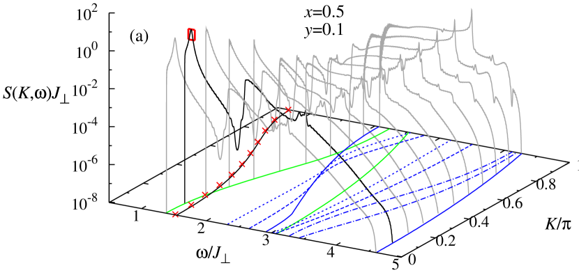
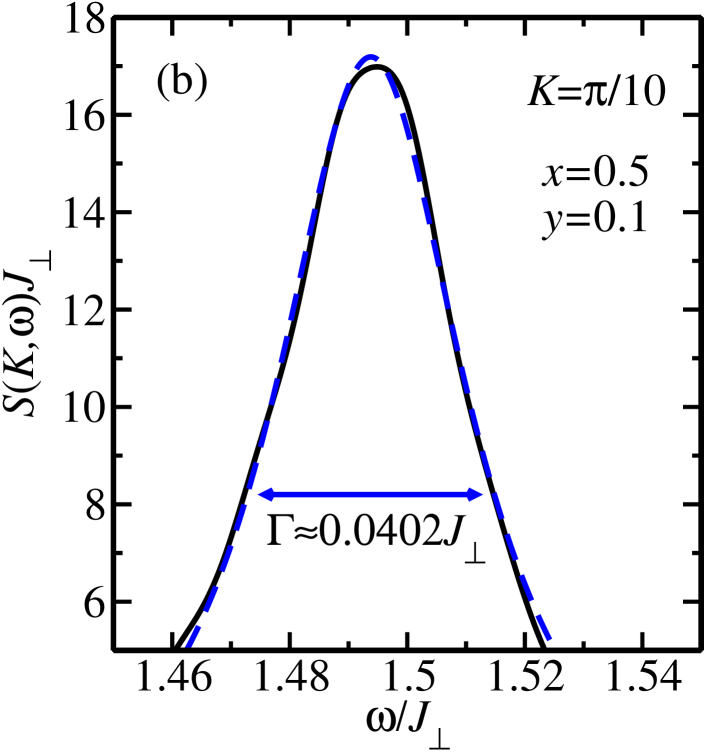
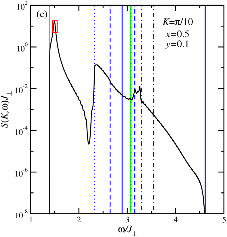
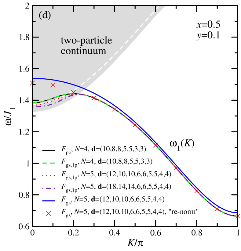
Figure 10: Spectral properties of the asymmetric spin-${1}/{2}$ ladder. Panels (a), (b) and (c) show the spectral density of the asymmetric spin-${1}/{2}$ ladder for $x=0.5$ and $y=0.1$. In Panel (b) a Lorentzian is fitted to the spectral density. The described quasiparticle exhibits a inverse lifetime of $\Gamma\approx 0.0402J_{\perp}$. Panel (d) compares the results of figure 8b with the red crosses depicting the renormalized one-triplon dispersion obtained by using the generator $F_{\textrm{gs}}(l)$ and (tri)diagonalization in the subspace (2.15abeeia)-(2.15abeeic). This renormalized one-triplon dispersion is also depicted in Panel (a).

To keep track of this spectral density we display the results presented in figure 9 also in the $\omega,K$-plane of figure 10a. For $K=0$ and $K={\pi}/{10}$ decaying triplons are observed. Their density lies in the vicinity of the approximate one-triplon dispersion. The region framed in red is shown in detail in figure 10b. In this region we can fit our data by a Lorentzian

$$L(\omega)=\frac{A}{\pi}\frac{\left({\Gamma}/{2}\right)^{2}}{\left(\omega-\omega_{0}\right)^{2}+{\left({\Gamma}/{2}\right)^{2}}}$$ (2.15abeeima)

with

$$A\approx 1.0848/J_{\perp}$$ (2.15abeeimb)

$$\omega_{0}\approx 1.4938J_{\perp}$$ (2.15abeeimc)

and the inverse lifetime

$$\Gamma\approx 0.0402J_{\perp}.$$ (2.15abeeimd)

For clarity, figure 10c shows the spectral density at $K={\pi}/{10}$ on logarithmic scale. Besides the strong one-triplon peak at $\omega_{0}\approx 1.4938J_{\perp}$ the spectral density increases distinctly at the beginning of the three-particle continuum involving the $S=0$ bound state. Another rise of the spectral density occurs at the upper end of the three-particle continuum involving the $S=1$ bound state. At the beginning of the three-particle continuum involving the $S=2$ anti-bound state the spectral density drops notably. This illustrates that the existence of bound and anti-bound states influences the form of the spectral density significantly. Note that an additional channel, for instance contributions from scattering states of a single triplon and a triplon-triplon bound state, does not always imply an increase of the spectral density. It may also lead to a significant decrease. We attribute this phenomenon to destructive interference. That means the additional channel interferes destructively with the already existing channel so that a net decrease is engendered.

Finally, we want to discuss the shift of the one-triplon dispersion caused by the hybridization of two- and three-particle states (cf. (2.15abeeia)-(2.15abeeic)). In the sequel we call this shifted one-triplon dispersion as the renormalized one-triplon dispersion. The results shown in figure 10d are partly those of figure 8b. In addition, the red crosses depict results obtained from a tridiagonalization after the CUT induced by $F_{\textrm{gs}}(l)$.

In the region of the Brillouin zone where the quasiparticles are well-defined we obtain the renormalized one-triplon dispersion by fixing the total momentum $K$ and calculating the lowest eigenvalue of the effective Hamiltonian $H_{\textrm{eff}}$ in the subspace (2.15abeeia)-(2.15abeeic). The results are represented in figure 10a and figure 10d by red crosses. To good accuracy, we retrieve the results obtained before by $F_{\textrm{pc}}(l)$ and $F_{\textrm{gs,1p}}(l)$ in the region without decay. Therefore, it is sufficient to consider the subspace (2.15abeeia)-(2.15abeeic) if one wants to describe the one-triplon dispersion of the asymmetric spin-${1}/{2}$ Heisenberg ladder with $x=0.5$ and $y=0.1$ by using the generator $F_{\textrm{gs}}(l)$.

Note that the calculation in the subspace (2.15abeeia)-(2.15abeeic) does not lead to the correct band edges of the triplon continuum because the shift of the one-triplon dispersion makes itself felt only if we included four-particle states as well. Hence this kind of calculation is not fully self-consistent. There are possibilities to achieve consistency between the one-triplon dispersion and the band edges of the continua. But this issue is beyond the scope of the present article.

In the region where the one-triplon dispersion hybridizes with the two-triplon continuum the red crosses shown in figure 10a and figure 10d indicate the energy with the maximum spectral intensity $S(K,\omega)$. These energies represent what is usually seen as the energy of a quasiparticle with finite life-time. The energies determined in this way lie between what is obtained from $F_{\textrm{gs}}(l)$ in the one-triplon sector (blue line in figure 10d) and what is obtained from $F_{\textrm{pc}}(l)$ or from $F_{\textrm{gs,1p}}(l)$.

We emphasize, that the advantage of the generator $F_{\textrm{gs}}(l)$ compared to the generator $F_{\textrm{gs,1p}}(l)$ or $F_{\textrm{pc}}(l)$ is that also the quasiparticle decay is described in the region of the Brillouin zone where the one-triplon dispersion merges with the two-triplon continuum. The generator $F_{\textrm{gs}}(l)$ avoids rearrangement processes during the flow which lead to a potentially misleading quasiparticle picture. Thereby the CUT becomes more robust. Hence the proposed adapted generator achieves the goal from the outset to describe decaying quasiparticles properly.

5 Summary

In the present paper, we introduced an approach based on continuous unitary transformations to describe systems with unstable quasiparticles. The main idea is to use a generator formulated in second quantization which leads to an effective model where only the ground state is isolated from the rest of the Hilbert space.

In the first part of this paper we described the properties of this adapted generator and discussed similarities and differences with other generators. Additionally, we derived the adapted generator in the context of variational calculations. All considerations were completely general and did neither depend on the model under study nor on the actual realization of the continuous unitary transformation. Thus we expect that generally an analogous modification of the unitary transformation can also be used in other approaches, for instance in high-order series expansions by orthogonal transformations [86], to capture resonant behavior. Not the life time will be accessible directly by a series, but the effective Hamiltonian. Then a subsequent analysis by variational methods (as presented in the present work) or by diagrammatic approaches has to be used.

In the second part of this paper we illustrated the theoretical deliberations for the asymmetric antiferromagnetic spin-${1}/{2}$ Heisenberg ladder. This model shows spontaneous triplon decay into two-triplon scattering states. The strength of this decay is controlled by the frustrating diagonal interaction $J_{\textrm{diag}}$. A more comprehensive study of this particular model is left to ongoing research.

We used the generator $F_{\textrm{gs}}(l)$ which only isolates the ground state and an additional Lanczos tridiagonalization in a variational subspace which consisted of states containing up to three triplons. We showed that in this way the resonance behavior of the decaying triplon can be described explicitly. The continuous unitary transformation was realized in a self-similar way.

In conclusion, we extended the range of applications of continuous unitary transformation to systems which exhibit unstable quasiparticles. We expect that an analogous extension can also be implemented for other unitary transformations.

Appendix A Ordering of the generator $F_{\textrm{pc}}(l)$

The generator $F_{\textrm{pc}}(l)$ sorts the eigenvalues $E_{i}$ in ascending order of the particle number $q_{i}$ of the corresponding eigenvectors such that $q_{i}>q_{j}\Rightarrow E_{i}>E_{j}$. Particularly, this implies that the vacuum state $\mathinner{|{0}\rangle}$ of the effective Hamiltonian represents the ground state of the system. In the following, we derive this statement.

In an eigenbasis of the operator $Q$, which counts the number of (quasi)particles of a given state, the generator $F_{\textrm{pc}}(l)$ is given by

$$\mathcal{F}_{i,j}(l)=\textrm{sgn}\left(q_{i}-q_{j}\right)\mathcal{H}_{i,j}(l),$$ (2.15abeeima)

where $q_{i}$ and $q_{j}$ are eigenvalues of the operator $Q$. In general the eigenspace for a given number of (quasi)particles $q_{i}$ has a large dimension which is infinite for infinite system size, but for the purpose of the present derivation we stick to finite dimensional Hilbert spaces. We use the convention that $\mathcal{H}_{i,j}(l)$ stands not only for a single matrix element but for the whole submatrix of the Hamiltonian $\mathcal{H}$ which connects the eigenspace belonging to the eigenvalue $q_{i}$ with the eigenspace belonging to the eigenvalue $q_{j}$. Therefore $\mathcal{H}_{i,j}(l)$ is given by a matrix with the dimension $D_{i}\times D_{j}$, where $D_{i}$ is the dimension of the eigenspace $Q=q_{i}$.

Using the generator (2.15abeeima) the general flow equation (2.1) yields the matrix equation

$$\eqalign{\partial_{l}\mathcal{H}_{i,j}(l)=-\textrm{sgn}\left(q_{i}-q_{j}\right)\left(\mathcal{H}_{i,i}(l)\mathcal{H}_{i,j}(l)-\mathcal{H}_{i,j}(l)\mathcal{H}_{j,j}(l)\right)\\ +\sum\limits_{k\neq i,j}\left(\textrm{sgn}\left(q_{i}-q_{k}\right)+\textrm{sgn}\left(q_{j}-q_{k}\right)\right)\mathcal{H}_{i,k}(l)\mathcal{H}_{k,j}(l).}$$ (2.15abeeimd)

Since the effective model will be block diagonal, all off-diagonal matrices $\mathcal{H}_{i,j}(l)$ with $i\neq j$ have to vanish for $l\rightarrow\infty$. Hence for large $l$ the equation (2.15abeeimd) is dominated by the first term on the right hand side where the off-diagonal matrices only appear linearly. So for large $l$ the asymptotic behavior of (2.15abeeimd) is given by

$$\partial_{l}\mathcal{H}_{i,j}(l)=-\textrm{sgn}\left(q_{i}-q_{j}\right)\left(\mathcal{H}_{i,i}\mathcal{H}_{i,j}(l)-\mathcal{H}_{i,j}(l)\mathcal{H}_{j,j}\right)+{\Or}\left(\mathcal{H}_{i,j}^{2}(l)\right).$$ (2.15abeeime)

Note that within this approximation $\partial_{l}\mathcal{H}_{i,i}(l)=0$ $\forall i$, so that we can neglect the $l$-dependence of $\mathcal{H}_{i,i}(l)$ and $\mathcal{H}_{j,j}(l)$. Without loss of generality we assume in the following that $q_{i}>q_{j}$. Then (2.15abeeime) yields

$$\partial_{l}\mathcal{H}_{i,j}(l)=-\left(\mathcal{H}_{i,i}\mathcal{H}_{i,j}(l)-\mathcal{H}_{i,j}(l)\mathcal{H}_{j,j}\right)+{\Or}\left(\mathcal{H}_{i,j}^{2}(l)\right).$$ (2.15abeeimf)

The matrix $\mathcal{H}_{i,i}$ and the matrix $\mathcal{H}_{j,j}$ are Hermitian, thus unitary transformations $\mathcal{U}_{i}$ and $\mathcal{U}_{j}$ exist which diagonalize $\mathcal{H}_{i,i}$ and $\mathcal{H}_{j,j}$, respectively. We will denote this diagonal matrices by $\mathcal{D}_{i}:=\mathcal{U}_{i}^{{\dagger}}\mathcal{H}_{i,i}\mathcal{U}_{i}$ and $\mathcal{D}_{j}:=\mathcal{U}_{j}^{{\dagger}}\mathcal{H}_{j,j}\mathcal{U}_{j}$. By multiplying (2.15abeeimf) from the left by $\mathcal{U}_{i}^{{\dagger}}$ and from the right by $\mathcal{U}_{j}$ one obtains

$$\partial_{l}\mathcal{\widetilde{H}}_{i,j}(l)=-\left(\mathcal{D}_{i}\mathcal{\widetilde{H}}_{i,j}(l)-\mathcal{\widetilde{H}}_{i,j}(l)\mathcal{D}_{j}\right)+{\Or}\left(\mathcal{\widetilde{H}}_{i,j}^{2}(l)\right),$$ (2.15abeeimg)

where $\mathcal{\widetilde{H}}_{i,j}(l):=\mathcal{U}_{i}^{{\dagger}}\mathcal{H}_{i,j}(l)\mathcal{U}_{j}$. According to (2.15abeeimg) the $(n,m)$ matrix element of $\mathcal{\widetilde{H}}_{i,j}(l)$ satisfies

$$\eqalign{\partial_{l}\left(\mathcal{\widetilde{H}}_{i,j}(l)\right)_{n,m}&=-\sum\limits_{k}\Big{(}\mathcal{D}_{i}\Big{)}_{n,k}\left(\mathcal{\widetilde{H}}_{i,j}(l)\right)_{k,m}+\sum\limits_{k}\left(\mathcal{\widetilde{H}}_{i,j}(l)\right)_{n,k}\left(\mathcal{D}_{j}\right)_{k,m}\\ &=-\left(\Big{(}\mathcal{D}_{i}\Big{)}_{n,n}-\left(\mathcal{D}_{j}\right)_{m,m}\right)\left(\mathcal{\widetilde{H}}_{i,j}(l)\right)_{n,m}}$$ (2.15abeeimj)

in linear order in the non-diagonal matrices. Since $\mathcal{H}_{i,j}(l)$ vanishes for $l\rightarrow\infty$, $\mathcal{\widetilde{H}}_{i,j}(l)$ must vanish as well. Therefore, for large $l$ the inequality

$$\Big{(}\mathcal{D}_{i}\Big{)}_{n,n}-\left(\mathcal{D}_{j}\right)_{m,m}>0$$ (2.15abeeimk)

must be fulfilled for all $n,m$ for which the matrix elements $(\mathcal{\widetilde{H}}_{i,j}(l))_{n,m}\nequiv 0$ are non-zero. This implies that all eigenvalues of $\mathcal{D}_{i}$ must be larger than the eigenvalues of $\mathcal{D}_{j}$. Thus, the eigenvalues are sorted in ascending order of the particle number of the corresponding eigenvectors, as asserted above.

Note that this ordering does not need to occur, if the corresponding eigenvectors are not connected to each other by a finite matrix element of the Hamiltonian for $l$ large, but not infinite. If $\mathcal{\widetilde{H}}_{i,j}(l)=0$ for all $l$ or for $l>l_{0}<\infty$ the argument to derive (2.15abeeimk) from (2.15abeeimj) does not hold. For example, this is the case when the system exhibits symmetries which prevent certain subspaces to be linked, as we see for the symmetric spin ladder.

Appendix B Transformation of subspaces

B.1 Ground state

In section 2.4 we argue that all generators $F_{\textrm{pc}}(l)$, $F_{\textrm{gs}}(l)$, $F_{\textrm{mgs}}(l)$, and $F_{\textrm{gs,1p}}(l)$) considered so far transform the vacuum state $\mathinner{|{0(l)}\rangle}$ in the same way if the flow equation is solved exactly. Here we prove this statement.

Previously, we defined the $l$-dependent Hamiltonian by $H(l):=U^{{\dagger}}(l)HU(l)$. Alternatively, we can keep the operators constant but make the states $l$-dependent. This is in complete analogy to passing from the Heisenberg picture to the Schrödinger picture. Hence, the $l$-dependence of the vacuum state is given by $\mathinner{|{0(l)}\rangle}=U(l)\mathinner{|{0}\rangle}$ and the generator is given by $F(l)=-U^{{\dagger}}(l)\left(\partial_{l}U(l)\right)$. Thus, for the derivative of $\mathinner{|{0(l)}\rangle}$ it follows

$$\eqalign{\partial_{l}\mathinner{|{0(l)}\rangle}&=\partial_{l}U(l)\mathinner{|{0}\rangle}\\ &=U(l)\underbrace{U^{{\dagger}}(l)\left(\partial_{l}U(l)\right)}_{=-F(l)}\mathinner{|{0}\rangle}\\ &=-U(l)F(l)\mathinner{|{0}\rangle}.}$$ (2.15abeeimd)

Introducing a basis $\left\{\mathinner{|{i}\rangle}\right\}$ yields

$$\eqalign{\partial_{l}\mathinner{|{0(l)}\rangle}=&-\sum_{i}U(l)\mathinner{|{i}\rangle}\underbrace{\mathinner{\langle{i}|}F(l)\mathinner{|{0}\rangle}}_{=F_{i,0}(l)}.}$$ (2.15abeeimf)

The key observation is that for all considered generators the matrix element $F_{i,0}(l)$ is the same, namely

$$F_{i,0}(l)=\cases{H_{i,0}(l)&for $i>0$\\ 0&for $i=0$}.$$ (2.15abeeimg)

Applying (2.15abeeimg) to (2.15abeeimf) yields

$$\eqalign{\partial_{l}\mathinner{|{0(l)}\rangle}&=-\sum_{i\neq 0}U(l)\mathinner{|{i}\rangle}\mathinner{\langle{i}|}H(l)\mathinner{|{0}\rangle}\\ &=-\left(\sum_{i}U(l)\mathinner{|{i}\rangle}\mathinner{\langle{i}|}H(l)\mathinner{|{0}\rangle}\right)+U(l)\mathinner{|{0}\rangle}\mathinner{\langle{0}|}H(l)\mathinner{|{0}\rangle}.}$$ (2.15abeeimj)

Shifting the $l$-dependency to the vacuum state and using the equality $U(l)U^{{\dagger}}(l)\equiv 1$ provides us with

$$\eqalign{\partial_{l}\mathinner{|{0(l)}\rangle}&=-H\mathinner{|{0(l)}\rangle}+\mathinner{|{0(l)}\rangle}\mathinner{\langle{0(l)}|}H\mathinner{|{0(l)}\rangle}\\ &=\Big{[}P_{0}(l),H\Big{]}\mathinner{|{0(l)}\rangle}}$$ (2.15abeeimm)

with the $l$-dependent projector $P_{0}(l)=\mathinner{|{0(l)}\rangle}\mathinner{\langle{0(l)}|}$. According to (2.15abeeimm) the derivative of $\mathinner{|{0(l)}\rangle}$ only depends on $\mathinner{|{0(l)}\rangle}$ itself and the initial Hamiltonian $H$. Therefore, the considered generators all transform the vacuum state $\mathinner{|{0(l)}\rangle}$ in the same way. The essential point of the proof is that for all considered generators the matrix elements $F_{i,0}(l)$ are defined identically by $(\ref{eq:def_g_i0})$. Note, however, that the statement, that all generators treat $\mathinner{|{0}\rangle}$ alike, does no longer hold if approximations (truncations) are introduced.

B.2 One-particle space

The proof presented in the previous subsection can be generalized. Since the action of the generator $F_{\textrm{pc}}(l)$ and the generator $F_{\textrm{gs,1p}}(l)$ is also the same on the one-particle subspace, one can prove that they also transform all one-particle states in the same way. In the following we characterize the states by their number of (quasi)particles, so it is useful to use an eigenbasis $\left\{\mathinner{|{i}\rangle}\right\}$ of the (quasi)particle number operator $Q$. The number of (quasi)particles of a state $\mathinner{|{i}\rangle}$ is denoted by $q_{i}$. Consider the derivative of all states with at most one particle

$$\eqalign{\partial_{l}\sum_{\makebox[0.0pt]{$\scriptstyle i:q_{i}\leq 1$}}\mathinner{|{i(l)}\rangle}&=\sum_{i:q_{i}\leq 1}\partial_{l}U(l)\mathinner{|{i}\rangle}\\ &=-\sum_{\makebox[0.0pt]{$\scriptstyle i:q_{i}\leq 1$}}U(l)F(l)\mathinner{|{i}\rangle}\\ &=-\sum_{\makebox[0.0pt]{$\scriptstyle i:q_{i}\leq 1,j$}}U(l)\mathinner{|{j}\rangle}\underbrace{\mathinner{\langle{j}|}F(l)\mathinner{|{i}\rangle}}_{=F_{j,i}(l)}.}$$ (2.15abeeimq)

For both generators the matrix elements $F_{j,i}(l)$ with $q_{i}\leq 1$ are given by

$$F_{j,i}(l)=\textrm{sgn}\left(q_{j}-q_{i}\right)H_{j,i}(l)$$ (2.15abeeimr)

according to (2.3) and (2.15v). Hence we have

$$\eqalign{\partial_{l}\sum_{i:q_{i}\leq 1}\mathinner{|{i(l)}\rangle}=-\sum_{\makebox[0.0pt]{$\scriptstyle i:q_{i}\leq 1,j:q_{j}>1$}}U(l)\mathinner{|{j}\rangle}{\mathinner{\langle{j}|}H(l)\mathinner{|{i}\rangle}}\\ -\sum_{\makebox[0.0pt]{$\scriptstyle i:q_{i}\leq 1,j:q_{j}\leq 1$}}\textrm{sgn}\left(q_{j}-q_{i}\right)U(l)\mathinner{|{j}\rangle}{\mathinner{\langle{j}|}H(l)\mathinner{|{i}\rangle}}}$$ (2.15abeeimu)

To the first part on the right hand side of (2.15abeeimu) we add all missing contributions with $q_{j}\leq 1$. Hence we arrive at

$$\eqalign{\partial_{l}\sum_{i:q_{i}\leq 1}\mathinner{|{i(l)}\rangle}=-\sum_{\makebox[0.0pt]{$\scriptstyle i:q_{i}\leq 1$}}U(l)H(l)\mathinner{|{i}\rangle}+\sum_{\makebox[0.0pt]{$\scriptstyle i:q_{i}\leq 1,j:q_{j}\leq 1$}}U(l)\mathinner{|{j}\rangle}{\mathinner{\langle{j}|}H(l)\mathinner{|{i}\rangle}}\\ -\sum_{\makebox[0.0pt]{$\scriptstyle i:q_{i}\leq 1,j:q_{j}\leq 1$}}\textrm{sgn}\left(q_{j}-q_{i}\right)U(l)\mathinner{|{j}\rangle}{\mathinner{\langle{j}|}H(l)\mathinner{|{i}\rangle}}.}$$ (2.15abeeimx)

Just as in the previous subsection we shift the $l$-dependence from the Hamiltonian $H(l)$ to the states

$$\eqalign{\partial_{l}\sum_{\makebox[0.0pt]{$\scriptstyle i:q_{i}\leq 1$}}\mathinner{|{i(l)}\rangle}=-\sum_{i:q_{i}\leq 1}H\mathinner{|{i(l)}\rangle}+\sum_{\makebox[0.0pt]{$\scriptstyle i:q_{i}\leq 1,j:q_{j}\leq 1$}}\mathinner{|{j(l)}\rangle}{\mathinner{\langle{j(l)}|}H\mathinner{|{i(l)}\rangle}}\\ -\sum_{\makebox[0.0pt]{$\scriptstyle i:q_{i}\leq 1,j:q_{j}\leq 1$}}\textrm{sgn}\left(q_{j}-q_{i}\right)\mathinner{|{j(l)}\rangle}{\mathinner{\langle{j(l)}|}H\mathinner{|{i(l)}\rangle}}.}$$ (2.15abeeimaa)

It follows that the transformation of the subspace $\left\{\mathinner{|{i}\rangle}\right\}$ with $q_{i}\leq 1$ is independent from all other states $\left\{\mathinner{|{i}\rangle}\right\}$ with $q_{i}>1$. The transformation only depends on the initial Hamiltonian $H$. Therefore, the generator $F_{\textrm{pc}}(l)$ and the generator $F_{\textrm{gs,1p}}(l)$ transform the one-particle subspace in the same way. Note that this proof is not restricted to the case $q_{i}\leq 1$ and can easily be adapted to the case $q_{i}\leq n\in\mathbb{N}$. The choice (2.15v) or (2.15abeeimr) has to be adapted accordingly, i.e., we have pass from $F_{\textrm{gs,1p}}(l)$ to $F_{\textrm{gs,$n$p}}(l)$ with

$$F_{\textrm{gs,$n$p}}(l)=\sum_{p=0}^{n}\sum_{i>p}^{N}\left(H_{p}^{i}(l)-H_{i}^{p}(l)\right).$$ (2.15abeeimab)

Appendix C Lanczos tridiagonalization

To determine the spectral density (2.15abeeg) one has to calculate the coefficients $a_{i}(K)$ and $b_{i}(K)$ of the continued fraction representation of the Green function (2.15abeeh). This can be done by the Lanczos recursion scheme, for which we restrict our calculations to the subspace (2.15abeeia)-(2.15abeeic). Within this subspace the recursion (Lanczos tridiagonalization)

$$\mathinner{|{\psi_{0}}\rangle}= \mathinner{|{K,z}\rangle}$$ (C.0a)

$$\mathinner{|{\psi_{1}}\rangle}= \left({H_{\textrm{eff}}^{\textrm{res}}-a_{0}(K)}\right)\mathinner{|{\psi_{0}}\rangle}$$ (C.0b)

$$\mathinner{|{\psi_{2}}\rangle}= \left({H_{\textrm{eff}}^{\textrm{res}}-a_{1}(K)}\right)\mathinner{|{\psi_{1}}\rangle}-b_{1}(K)^{2}\mathinner{|{\psi_{0}}\rangle}$$ (C.0c)

$$\mathinner{|{\psi_{3}}\rangle}= \left({H_{\textrm{eff}}^{\textrm{res}}-a_{2}(K)}\right)\mathinner{|{\psi_{2}}\rangle}-b_{2}(K)^{2}\mathinner{|{\psi_{1}}\rangle}$$ (C.0d)

$$\vdots$$

with

$$a_{i}(K) =\frac{\mathinner{\langle{\psi_{i}}|}H_{\textrm{eff}}^{\textrm{res}}\mathinner{|{\psi_{i}}\rangle}}{\mathinner{\langle{\psi_{i}|\psi_{i}}\rangle}}\qquad \textrm{for }i=0,1,2,\ldots$$ (C.0e)

$$b_{i}(K)^{2} =\frac{\mathinner{\langle{\psi_{i}|\psi_{i}}\rangle}}{\mathinner{\langle{\psi_{i-1}|\psi_{i-1}}\rangle}}\qquad \textrm{for }i=1,2,3,\ldots$$ (C.0f)

$$b_{0}(K) =0$$ (C.0g)

generates a set of orthogonal states $\mathinner{|{\psi_{i}}\rangle}$. The action of the restricted Hamiltonian (2.15abeeil) in the three-particles subspace (2.15abeeia)-(2.15abeeic) is given in section D. In the generated basis $\left\{\mathinner{|{\psi_{i}}\rangle}\right\}$ the matrix of the restricted effective Hamiltonian $H_{\textrm{eff}}^{\textrm{res}}$ is tridiagonal, where the $a_{i}(K)$ are the diagonal matrix elements and the $b_{i}(K)$ are the elements on the second diagonal. All other matrix elements are zero.

Figure 11 shows the results for the coefficients $a_{i}(K)$ and $b_{i}(K)$ for $x=0.5$, $y=0.1$ and $K={\pi}/{10}$.

Figure 11: Continued fraction coefficients $a_{i}(K)$ and $b_{i}(K)$ for $x=0.5$, $y=0.1$ and momentum $K={\pi}/{10}$. The restriction of the considered subspace becomes conspicuous at $i\approx 115$.

First it appears that both coefficients $a_{i}(K)$ and $b_{i}(K)$ ($i\lessapprox 115$) converge to fixed values $a_{\infty}(K)$ and $b_{\infty}(K)$ as it should be for a bounded and gapless spectral density of an infinitely large system [84]. But for $i\gtrapprox 115$ both coefficients start to change their values again noticeably. This is a consequence of the fact that we had to restrict the relative distances $d$ and $d_{1}+d_{2}$ to a maximum of $119$ rungs (cf. (2.15abeeia)-(2.15abeeic)) in our numerical calculations. Therefore, we only use the first 100 coefficients and terminate the continued fraction at $i=100$ as described in the following subsection.

C.1 Termination

The spectral density $S(K,\omega)$ at fixed $K$ as obtained by a finite continued fraction of the Green function (2.15abeeh) has poles at the zeros of the denominator. Thus, the spectral density $S(K,\omega)$ is a collection of $\delta$-peaks. One standard approach to obtain a continuous density is to introduce a slight broadening of $S(K,\omega)$ via $\omega\rightarrow\omega+\rmi\delta$ with a small real number $\delta$. This procedure corresponds to smearing out $\delta$-peaks as Lorentzian functions of width $\delta$. The caveat is that also all truly sharp features such as band edges or van Hove sigularities are smeared out. However, a notably improved resolution of $S(K,\omega)$ can be achieved by introducing an appropriate termination of the continued fraction.

If we want to evaluate the continued fraction for the infinite large system, we have to stop our recursion before the finiteness of the considered subspace (2.15abeeia)-(2.15abeeic) becomes conspicuous. Therefore, we compute the average value of $a_{i}(K)$ and $b_{i}(K)$ for $i=80\ldots 100$ (cf. figure 11) to obtain a good approximation for the limits $a_{\infty}(K)$ and $b_{\infty}(K)$. From these limits the upper and lower boundaries $E_{\textrm{u}}(K)$ and $E_{\textrm{l}}(K)$ of the spectral density $S(K,\omega)$ are determined via [84]

$$E_{\textrm{u}}(K)= a_{\infty}(K)+2b_{\infty}(K)$$ (C.0a)

$$E_{\textrm{l}}(K)= a_{\infty}(K)-2b_{\infty}(K)\ .$$ (C.0b)

The existence of an upper boundary of the spectral density is a consequence of our restriction to a subspace which contains three quasiparticles at maximum. Finally, we use the directly calculated coefficients $a_{i}(K)$ and $b_{i+1}(K)$ for $i=0\ldots 99$ and subsequently the square root terminator defined by the approximate limits $a_{\infty}(K)$ and $b_{\infty}(K)$. By doing this, we assume that all following coefficients $a_{i}(K)$ and $b_{i+1}(K)$ with $i\geq 100$ are constant. The square root terminator $T(K)$ is given by

$$T =\frac{1}{2b_{\infty}^{2}}\left(\omega-a_{\infty}-\sqrt{-D}\right)\qquad \textrm{for }\omega\geq E_{\textrm{u}}$$ (C.0a)

$$T =\frac{1}{2b_{\infty}^{2}}\left(\omega-a_{\infty}-\rmi\sqrt{D}\right)\qquad \textrm{for }E_{\textrm{l}}\leq\omega\leq E_{\textrm{u}}$$ (C.0b)

$$T =\frac{1}{2b_{\infty}^{2}}\left(\omega-a_{\infty}+\sqrt{-D}\right)\qquad \textrm{for }\omega\leq E_{\textrm{l}}$$ (C.0c)

with

$$D=4b_{\infty}^{2}-\left(\omega-a_{\infty}\right)^{2}\ ,$$ (C.0d)

where we suppressed all $K$ dependences for the sake of simplicity. The last considered coefficient $b_{100}(K)$ in (2.15abeeh) is multiplied by the appropriate terminator $T(K)$. The imaginary part of the resulting expression yields the continuous part of the spectral density $S(K,\omega)$. In this way we can reliably approximate the thermodynamic limit of the spectral density $S(K,\omega)$ by calculations in a finite subspace.

Appendix D Analysis of the effective model

Here we present details of the analysis of the effective Hamiltonians for the asymmetric ladder generated by CUTs. More details are given in [87, 56, 88] for the special case of a particle conserving effective Hamiltonian.

The generators $F_{\textrm{pc}}(l)$ and $F_{\textrm{gs,1p}}(l)$ isolate the one-particle subspace from all other subspaces (cf. figure 2a and figure 2c). Therefore, the one-particle eigenvalues can be calculated without considering states with a higher particle number.

The effective Hamiltonians obtained by the generator $F_{\textrm{gs}}(l)$ still contain interactions between the one-particle subspace and other subspaces (cf. figure 2b). Consequently, a diagonalization in the one-particle subspace only gives an approximation for the eigenvalues of the effective Hamiltonian, namely an upper bound for the eigenvalues if the ground state energy is sufficiently well described. The results for the eigenvalues can be improved by considering higher particle subspaces as well (see figure 12).

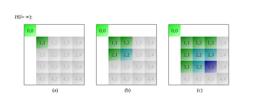
Figure 12: (Color online) Considered subspaces to analyze the effective Hamiltonian obtained by the generator $F_{\textrm{gs}}(l)$. The generator $F_{\textrm{gs}}(l)$ only isolates the part $H_{0}^{0}(l)$. Colored blocks illustrate interactions which are included. Grey blocks illustrate neglected interactions. Panel (a) describes an analysis within the one-triplon subspace. Panel (b) describes an analysis within the one- and two-triplon subspace. Panel (c) describes an analysis within the one-, two- and three-triplon subspace, see (2.15abeeia)-(2.15abeeic)

In this paper we consider subspaces which consist of states which contain up to three triplons.

The Fourier transformed one-, two- and three-particle states are given by (2.15abeeia)-(2.15abeeic). In any practical calculation the relative distances must be truncated to make the subspace finite. Note that due to the hard-core algebra it is not possible that two particles occupy the same rung. Below the action of the various parts of the effective Hamiltonians are given.

D.1 $H_{1}^{1}$

The action of the operator $H_{1}^{1}$ on the one-triplon state $\mathinner{|{K,\alpha}\rangle}$ is given by

$$H_{1}^{1}\mathinner{|{K,\alpha}\rangle}= \sum_{{r},\alpha^{\prime}}\rme^{\rmi K{r}}c_{11;{r}}^{\alpha^{\prime},\alpha}\mathinner{|{K,\alpha^{\prime}}\rangle}$$ (D.1)

with

$$c_{11;{r}}^{\alpha^{\prime},\alpha}:= \mathinner{\langle{R,\alpha^{\prime}}|}H_{1}^{1}\mathinner{|{R+r,\alpha}\rangle}$$ (D.2)

and $R\in\mathbb{Z}$. Note that due to the translational symmetry only the relative distance $r$ between the states $\mathinner{|{R,\alpha^{\prime}}\rangle}$ and $\mathinner{|{R+r,\alpha}\rangle}$ occurs in the coefficient $c_{11;{r}}^{\alpha^{\prime},\alpha}$. In the special case of a SU(2) symmetric Hamiltonian the coefficients $c_{11;{r}}^{\alpha^{\prime},\alpha}$ obey the relation $c_{11;{r}}^{\alpha^{\prime},\alpha}=\delta_{\alpha^{\prime},\alpha}c_{11;r}$. The used truncation scheme (cf. section 3.1) causes $c_{11;{r}}^{\alpha^{\prime},\alpha}=0$ for $|r|>d_{2}$. All other coefficients $c$ which appear in the following are affected by the truncation scheme in an analogous way.

The action of the operator $H_{1}^{1}$ on the two-triplon state $\mathinner{|{K,\alpha}\rangle}\mathinner{|{d,\beta}\rangle}$ is given by

$$H_{1}^{1}\mathinner{|{K,\alpha}\rangle}\mathinner{|{d,\beta}\rangle}=\sum_{\makebox[0.0pt]{$\scriptstyle{r}>-d\atop\alpha^{\prime}$}}c_{11;{r}}^{\alpha^{\prime},\alpha}\rme^{\rmi K\frac{{r}}{2}}\mathinner{|{K,\alpha^{\prime}}\rangle}\mathinner{|{{r}+d,\beta}\rangle}$$ (D.0a)

$$+\sum_{\makebox[0.0pt]{$\scriptstyle{r}<-d\atop\alpha^{\prime}$}}c_{11;{r}}^{\alpha^{\prime},\alpha}\rme^{\rmi K\frac{{r}}{2}}\mathinner{|{K,\beta}\rangle}\mathinner{|{-\left({r}+d\right),\alpha^{\prime}}\rangle}$$ (D.0b)

$$+\sum_{\makebox[0.0pt]{$\scriptstyle{r}<d\atop\beta^{\prime}$}}c_{11;{r}}^{\beta^{\prime},\beta}\rme^{\rmi K\frac{{r}}{2}}\mathinner{|{K,\alpha}\rangle}\mathinner{|{-\left({r}-d\right),\beta^{\prime}}\rangle}$$ (D.0c)

$$+\sum_{\makebox[0.0pt]{$\scriptstyle{r}>d\atop\beta^{\prime}$}}c_{11;{r}}^{\beta^{\prime},\beta}\rme^{\rmi K\frac{{r}}{2}}\mathinner{|{K,\beta^{\prime}}\rangle}\mathinner{|{r-d,\alpha}\rangle}$$ (D.0d)

The action of the operator $H_{1}^{1}$ on the three-triplon state $\mathinner{|{K,\alpha}\rangle}\mathinner{|{d_{1},\beta}\rangle}\mathinner{|{d_{2},\gamma}\rangle}$ is given by

$$H_{1}^{1}\mathinner{|{K,\alpha}\rangle}\mathinner{|{d_{1},\beta}\rangle}\mathinner{|{d_{2},\gamma}\rangle}=\sum_{\makebox[0.0pt]{$\scriptstyle{r}>-d_{1}\atop\alpha^{\prime}$}}c_{11;{r}}^{\alpha^{\prime},\alpha}\rme^{\rmi K\frac{{r}}{3}}\mathinner{|{K,\alpha^{\prime}}\rangle}\mathinner{|{{r}+d_{1},\beta}\rangle}\mathinner{|{d_{2},\gamma}\rangle}$$ (D.0a)

$$+\sum_{\makebox[0.0pt]{$\scriptstyle-(d_{1}+d_{2})<{r}<-d_{1}\atop\alpha^{\prime}$}}c_{11;{r}}^{\alpha^{\prime},\alpha}\rme^{\rmi K\frac{{r}}{3}}\mathinner{|{K,\beta}\rangle}\mathinner{|{-\left({r}+d_{1}\right),\alpha^{\prime}}\rangle}\mathinner{|{{r}+d_{1}+d_{2},\gamma}\rangle}$$ (D.0b)

$$+\sum_{\makebox[0.0pt]{$\scriptstyle{r}<-(d_{1}+d_{2})\atop\alpha^{\prime}$}}c_{11;{r}}^{\alpha^{\prime},\alpha}\rme^{\rmi K\frac{{r}}{3}}\mathinner{|{K,\beta}\rangle}\mathinner{|{d_{2},\gamma}\rangle}\mathinner{|{-\left({r}+d_{1}+d_{2}\right),\alpha^{\prime}}\rangle}$$ (D.0c)

$$+\sum_{\makebox[0.0pt]{$\scriptstyle-d_{2}<{r}<d_{1}\atop\beta^{\prime}$}}c_{11;{r}}^{\beta^{\prime},\beta}\rme^{\rmi K\frac{{r}}{3}}\mathinner{|{K,\alpha}\rangle}\mathinner{|{-({r}-d_{1}),\beta^{\prime}}\rangle}\mathinner{|{{r}+d_{2},\gamma}\rangle}$$ (D.0d)

$$+\sum_{\makebox[0.0pt]{$\scriptstyle{r}>d_{1}\atop\beta^{\prime}$}}c_{11;{r}}^{\beta^{\prime},\beta}\rme^{\rmi K\frac{{r}}{3}}\mathinner{|{K,\beta^{\prime}}\rangle}\mathinner{|{{r}-d_{1},\alpha}\rangle}\mathinner{|{d_{1}+d_{2},\gamma}\rangle}$$ (D.0e)

$$+\sum_{\makebox[0.0pt]{$\scriptstyle{r}<-d_{2}\atop\beta^{\prime}$}}c_{11;{r}}^{\beta^{\prime},\beta}\rme^{\rmi K\frac{{r}}{3}}\mathinner{|{K,\alpha}\rangle}\mathinner{|{d_{1}+d_{2},\gamma}\rangle}\mathinner{|{-\left({r}+d_{2}\right),\beta^{\prime}}\rangle}$$ (D.0f)

$$+\sum_{\makebox[0.0pt]{$\scriptstyle{r}<d_{2}\atop\gamma^{\prime}$}}c_{11;{r}}^{\gamma^{\prime},\gamma}\rme^{\rmi K\frac{{r}}{3}}\mathinner{|{K,\alpha}\rangle}\mathinner{|{d_{1},\beta}\rangle}\mathinner{|{-\left({r}-d_{2}\right),\gamma^{\prime}}\rangle}$$ (D.0g)

$$+\sum_{\makebox[0.0pt]{$\scriptstyle d_{2}<{r}<d_{1}+d_{2}\atop\gamma^{\prime}$}}c_{11;{r}}^{\gamma^{\prime},\gamma}\rme^{\rmi K\frac{{r}}{3}}\mathinner{|{K,\alpha}\rangle}\mathinner{|{-\left({r}-d_{1}-d_{2}\right),\gamma^{\prime}}\rangle}\mathinner{|{{r}-d_{2},\beta}\rangle}$$ (D.0h)

$$+\sum_{\makebox[0.0pt]{$\scriptstyle{r}>d_{1}+d_{2}\atop\gamma^{\prime}$}}c_{11;{r}}^{\gamma^{\prime},\gamma}\rme^{\rmi K\frac{{r}}{3}}\mathinner{|{K,\gamma^{\prime}}\rangle}\mathinner{|{{r}-d_{1}-d_{2},\alpha}\rangle}\mathinner{|{d_{1},\beta}\rangle}$$ (D.0i)

D.2 $H_{1}^{2}$

The action of the operator $H_{1}^{2}$ on the one-triplon state $\mathinner{|{K,\alpha}\rangle}$ is given by

$$H_{1}^{2}\mathinner{|{K,\alpha}\rangle}= \sum_{\makebox[0.0pt]{$\scriptstyle{r},d^{\prime}\atop\alpha^{\prime},\beta^{\prime}$}}c_{21;{r},d^{\prime}}^{\alpha^{\prime},\beta^{\prime},\alpha}\rme^{\rmi K\left({r}-\frac{d^{\prime}}{2}\right)}\mathinner{|{K,\alpha^{\prime}}\rangle}\mathinner{|{d^{\prime},\beta^{\prime}}\rangle}$$ (D.1)

with

$$c_{21;r,d^{\prime}}^{\alpha^{\prime},\beta^{\prime},\alpha}:= \mathinner{\langle{R,\alpha^{\prime}}|}\mathinner{\langle{R+d^{\prime},\beta^{\prime}}|}H_{1}^{2}\mathinner{|{{R+r},\alpha}\rangle}.$$ (D.2)

The action of the operator $H_{1}^{2}$ on the two-triplon state $\mathinner{|{K,\alpha}\rangle}\mathinner{|{d,\beta}\rangle}$ is given by

$$H_{1}^{2}\mathinner{|{K,\alpha}\rangle}\mathinner{|{d,\beta}\rangle}=\sum_{\makebox[0.0pt]{$\scriptstyle{r}>-d+d^{\prime}\atop d^{\prime},\alpha^{\prime},\gamma^{\prime}$}}c_{21;{r},d^{\prime}}^{\alpha^{\prime},\gamma^{\prime},\alpha}\rme^{\rmi K\left(\frac{4{r}+d-2d^{\prime}}{6}\right)}\mathinner{|{K,\alpha^{\prime}}\rangle}\mathinner{|{d^{\prime},\gamma^{\prime}}\rangle}\mathinner{|{{r}+d-d^{\prime},\beta}\rangle}$$ (D.0a)

$$+\sum_{\makebox[0.0pt]{$\scriptstyle-d<{r}<-d+d^{\prime}\atop d^{\prime},\alpha^{\prime},\gamma^{\prime}$}}c_{21;{r},d^{\prime}}^{\alpha^{\prime},\gamma^{\prime},\alpha}\rme^{\rmi K\left(\frac{4{r}+d-2d^{\prime}}{6}\right)}\mathinner{|{K,\alpha^{\prime}}\rangle}\mathinner{|{r+d,\beta}\rangle}\mathinner{|{-\left({r}+d\right)+d^{\prime},\gamma^{\prime}}\rangle}$$ (D.0b)

$$+\sum_{\makebox[0.0pt]{$\scriptstyle{r}<-d\atop d^{\prime},\alpha^{\prime},\gamma^{\prime}$}}c_{21;{r},d^{\prime}}^{\alpha^{\prime},\gamma^{\prime},\alpha}\rme^{\rmi K\left(\frac{4{r}+d-2d^{\prime}}{6}\right)}\mathinner{|{K,\beta}\rangle}\mathinner{|{-\left({r}+d\right),\alpha^{\prime}}\rangle}\mathinner{|{d^{\prime},\gamma^{\prime}}\rangle}$$ (D.0c)

$$+\sum_{\makebox[0.0pt]{$\scriptstyle{r}<d\atop d^{\prime},\beta^{\prime},\gamma^{\prime}$}}c_{21;{r},d^{\prime}}^{\beta^{\prime},\gamma^{\prime},\beta}\rme^{\rmi K\left(\frac{4{r}-d-2d^{\prime}}{6}\right)}\mathinner{|{K,\alpha}\rangle}\mathinner{|{-{r}+d,\beta^{\prime}}\rangle}\mathinner{|{d^{\prime},\gamma^{\prime}}\rangle}$$ (D.0d)

$$+\sum_{\makebox[0.0pt]{$\scriptstyle d<{r}<d+d^{\prime}\atop d^{\prime},\beta^{\prime},\gamma^{\prime}$}}c_{21;{r},d^{\prime}}^{\beta^{\prime},\gamma^{\prime},\beta}\rme^{\rmi K\left(\frac{4{r}-d-2d^{\prime}}{6}\right)}\mathinner{|{K,\beta^{\prime}}\rangle}\mathinner{|{{r}-d,\alpha}\rangle}\mathinner{|{-{r}+d+d^{\prime},\gamma^{\prime}}\rangle}$$ (D.0e)

$$+\sum_{\makebox[0.0pt]{$\scriptstyle{r}>d+d^{\prime}\atop d^{\prime},\beta^{\prime},\gamma^{\prime}$}}c_{21;{r},d^{\prime}}^{\beta^{\prime},\gamma^{\prime},\beta}\rme^{\rmi K\left(\frac{4{r}-d-2d^{\prime}}{6}\right)}\mathinner{|{K,\beta^{\prime}}\rangle}\mathinner{|{d^{\prime},\gamma^{\prime}}\rangle}\mathinner{|{{r}-\left(d+d^{\prime}\right),\alpha}\rangle}$$ (D.0f)

D.3 $H_{2}^{1}$

The action of the operator $H_{2}^{1}$ on the two-triplon state $\mathinner{|{K,\alpha}\rangle}\mathinner{|{d,\beta}\rangle}$ is given by

$$H_{2}^{1}\mathinner{|{K,\alpha}\rangle}\mathinner{|{d,\beta}\rangle}= \sum_{{r},\alpha^{\prime}}c_{12;{r},d}^{\alpha^{\prime},\alpha,\beta}\rme^{\rmi K\left({r}+\frac{d}{2}\right)}\mathinner{|{K,\alpha^{\prime}}\rangle}$$ (D.1)

with

$$c_{12;r,d}^{\alpha^{\prime},\alpha,\beta}:= \mathinner{\langle{R,\alpha^{\prime}}|}H_{2}^{1}\mathinner{|{R+{r},\alpha}\rangle}\mathinner{|{R+{r}+d,\beta}\rangle}.$$ (D.2)

The action of the operator $H_{2}^{1}$ on the three-triplon state $\mathinner{|{K,\alpha}\rangle}\mathinner{|{d_{1},\beta}\rangle}\mathinner{|{d_{2},\gamma}\rangle}$ is given by

$$H_{2}^{1}\mathinner{|{K,\alpha}\rangle}\mathinner{|{d_{1},\beta}\rangle}\mathinner{|{d_{2},\gamma}\rangle}=\sum_{\makebox[0.0pt]{$\scriptstyle{r}>-\left(d_{1}+d_{2}\right)\atop\alpha^{\prime}$}}c_{12;{r},d_{1}}^{\alpha^{\prime},\alpha,\beta}\rme^{\rmi K\left(\frac{3{r}+d_{1}-d_{2}}{6}\right)}\mathinner{|{K,\alpha^{\prime}}\rangle}\mathinner{|{{r}+d_{1}+d_{2},\gamma}\rangle}$$ (D.0a)

$$+\sum_{\makebox[0.0pt]{$\scriptstyle{r}<-\left(d_{1}+d_{2}\right)\atop\alpha^{\prime}$}}c_{12;{r},d_{1}}^{\alpha^{\prime},\alpha,\beta}\rme^{\rmi K\left(\frac{3{r}+d_{1}-d_{2}}{6}\right)}\mathinner{|{K,\gamma}\rangle}\mathinner{|{-\left({r}+d_{1}+d_{2}\right),\alpha^{\prime}}\rangle}$$ (D.0b)

$$+\sum_{\makebox[0.0pt]{$\scriptstyle{r}<d_{1}\atop\beta^{\prime}$}}c_{12;{r},d_{2}}^{\beta^{\prime},\beta,\gamma}\rme^{\rmi K\left(\frac{3{r}+d_{1}+2d_{2}}{6}\right)}\mathinner{|{K,\alpha}\rangle}\mathinner{|{-{r}+d_{1},\beta^{\prime}}\rangle}$$ (D.0c)

$$+\sum_{\makebox[0.0pt]{$\scriptstyle{r}>d_{1}\atop\beta^{\prime}$}}c_{12;{r},d_{2}}^{\beta^{\prime},\beta,\gamma}\rme^{\rmi K\left(\frac{3{r}+d_{1}+2d_{2}}{6}\right)}\mathinner{|{K,\beta^{\prime}}\rangle}\mathinner{|{{r}-d_{1},\alpha}\rangle}$$ (D.0d)

$$+\sum_{\makebox[0.0pt]{$\scriptstyle{r}>-d_{1}\atop\alpha^{\prime}$}}c_{12;{r},d_{1}+d_{2}}^{\alpha^{\prime},\alpha,\gamma}\rme^{\rmi K\left(\frac{3{r}+d_{1}+2d_{2}}{6}\right)}\mathinner{|{K,\alpha^{\prime}}\rangle}\mathinner{|{{r}+d_{1},\beta}\rangle}$$ (D.0e)

$$+\sum_{\makebox[0.0pt]{$\scriptstyle{r}<-d_{1}\atop\alpha^{\prime}$}}c_{12;{r},d_{1}+d_{2}}^{\alpha^{\prime},\alpha,\gamma}\rme^{\rmi K\left(\frac{3{r}+d_{1}+2d_{2}}{6}\right)}\mathinner{|{K,\beta}\rangle}\mathinner{|{-\left({r}+d_{1}\right),\alpha^{\prime}}\rangle}$$ (D.0f)

D.4 $H_{1}^{3}$

The action of the operator $H_{1}^{3}$ on the one-triplon state $\mathinner{|{K,\alpha}\rangle}$ is given by

$$H_{1}^{3}\mathinner{|{K,\alpha}\rangle}= \sum_{\makebox[0.0pt]{$\scriptstyle{r},d_{1}^{\prime},d_{2}^{\prime}\atop\alpha^{\prime},\beta^{\prime},\gamma^{\prime}$}}c_{31;{r},d_{1}^{\prime},d_{2}^{\prime}}^{\alpha^{\prime},\beta^{\prime},\gamma^{\prime},\alpha}\rme^{\rmi K\left({r}-\frac{2d_{1}^{\prime}+d_{2}^{\prime}}{3}\right)}\mathinner{|{K,\alpha^{\prime}}\rangle}\mathinner{|{d_{1}^{\prime},\beta^{\prime}}\rangle}\mathinner{|{d_{2}^{\prime},\gamma^{\prime}}\rangle}$$ (D.1)

with

$$c_{31;{r},d_{1}^{\prime},d_{2}^{\prime}}^{\alpha^{\prime},\beta^{\prime},\gamma^{\prime},\alpha}:=\mathinner{\langle{R,\alpha^{\prime}}|}\mathinner{\langle{R+d_{1}^{\prime},\beta^{\prime}}|}\mathinner{\langle{R+d_{1}^{\prime}+d_{2}^{\prime},\gamma^{\prime}}|}H_{1}^{3}\mathinner{|{{R+r},\alpha}\rangle}.$$ (D.2)

D.5 $H_{3}^{1}$

The action of the operator $H_{3}^{1}$ on the three-triplon state $\mathinner{|{K,\alpha}\rangle}\mathinner{|{d_{1},\beta}\rangle}\mathinner{|{d_{2},\gamma}\rangle}$ is given by

$$H_{3}^{1}\mathinner{|{K,\alpha}\rangle}\mathinner{|{d_{1},\beta}\rangle}\mathinner{|{d_{2},\gamma}\rangle}= \sum_{{r},\alpha^{\prime}}c_{13;{r},d_{1},d_{2}}^{\alpha^{\prime},\alpha,\beta,\gamma}\rme^{\rmi K\left({r}+\frac{2d_{1}+d_{2}}{3}\right)}\mathinner{|{K,\alpha^{\prime}}\rangle}$$ (D.3)

with

$$c_{13;r,d_{1},d_{2}}^{\alpha^{\prime},\alpha,\beta,\gamma}:=\mathinner{\langle{R,\alpha^{\prime}}|}H_{3}^{1}\mathinner{|{R+{r},\alpha}\rangle}\mathinner{|{R+{r}+d_{1},\beta}\rangle}\mathinner{|{R+r+d_{1}+d_{2},\gamma}\rangle}.$$ (D.4)

D.6 $H_{2}^{2}$

The action of the operator $H_{2}^{2}$ on the two-triplon state $\mathinner{|{K,\alpha}\rangle}\mathinner{|{d,\beta}\rangle}$ is given by

$$H_{2}^{2}\mathinner{|{K,\alpha}\rangle}\mathinner{|{d,\beta}\rangle}= \sum_{\makebox[0.0pt]{$\scriptstyle r,d^{\prime}\atop\alpha^{\prime},\beta^{\prime}$}}c_{22;{r},d^{\prime},d}^{\alpha^{\prime},\beta^{\prime},\alpha,\beta}\rme^{\rmi K\left({r}+\frac{d-d^{\prime}}{2}\right)}\mathinner{|{K,\alpha^{\prime}}\rangle}\mathinner{|{d^{\prime},\beta^{\prime}}\rangle}$$ (D.5)

with

$$c_{22;{r},d^{\prime},d}^{\alpha^{\prime},\beta^{\prime},\alpha,\beta}:= \mathinner{\langle{R,\alpha^{\prime}}|}\mathinner{\langle{R+d^{\prime},\beta^{\prime}}|}H_{2}^{2}\mathinner{|{R+r,\alpha}\rangle}\mathinner{|{R+r+d,\beta}\rangle}.$$ (D.6)

The action of the operator $H_{2}^{2}$ on the three-triplon state $\mathinner{|{K,\alpha}\rangle}\mathinner{|{d_{1},\beta}\rangle}\mathinner{|{d_{2},\gamma}\rangle}$ is given by

$$H_{2}^{2}\mathinner{|{K,\alpha}\rangle}\mathinner{|{d_{1},\beta}\rangle}\mathinner{|{d_{2},\gamma}\rangle}=\sum_{\makebox[0.0pt]{$\scriptstyle{r}>-\left(d_{1}+d_{2}\right)+d_{1}^{\prime}\atop d_{1}^{\prime},\alpha^{\prime},\beta^{\prime}$}}c_{22;{r},d_{1}^{\prime},d_{1}}^{\alpha^{\prime},\beta^{\prime},\alpha,\beta}\rme^{\rmi K\left(\frac{2{r}+d_{1}-d_{1}^{\prime}}{3}\right)}\mathinner{|{K,\alpha^{\prime}}\rangle}\mathinner{|{d_{1}^{\prime},\beta^{\prime}}\rangle}\mathinner{|{{r}+d_{1}+d_{2}-d_{1}^{\prime},\gamma}\rangle}$$ (D.0a)

$${+}\sum_{\makebox[0.0pt]{$\scriptstyle-\left(d_{1}+d_{2}\right)<{r}<-\left(d_{1}+d_{2}\right)+d_{1}^{\prime}\atop d_{1}^{\prime},\alpha^{\prime},\beta^{\prime}$}}c_{22;{r},d_{1}^{\prime},d_{1}}^{\alpha^{\prime},\beta^{\prime},\alpha,\beta}\rme^{\rmi K\left(\frac{2{r}+d_{1}-d_{1}^{\prime}}{3}\right)}\mathinner{|{K,\alpha^{\prime}}\rangle}\mathinner{|{{r}+d_{1}+d_{2},\gamma}\rangle}\mathinner{|{-\left({r}+d_{1}+d_{2}\right)+d_{1}^{\prime},\beta^{\prime}}\rangle}$$ (D.0b)

$${+}\sum_{\makebox[0.0pt]{$\scriptstyle{r}<-\left(d_{1}+d_{2}\right)\atop d_{1}^{\prime},\alpha^{\prime},\beta^{\prime}$}}c_{22;{r},d_{1}^{\prime},d_{1}}^{\alpha^{\prime},\beta^{\prime},\alpha,\beta}\rme^{\rmi K\left(\frac{2{r}+d_{1}-d_{1}^{\prime}}{3}\right)}\mathinner{|{K,\gamma}\rangle}\mathinner{|{-\left({r}+d_{1}+d_{2}\right),\alpha^{\prime}}\rangle}\mathinner{|{d_{1}^{\prime},\beta^{\prime}}\rangle}$$ (D.0c)

$$+\sum_{\makebox[0.0pt]{$\scriptstyle-d_{1}<{r}<d_{2}^{\prime}\atop d_{2}^{\prime},\alpha^{\prime},\gamma^{\prime}$}}c_{22;{r},d_{1}+d_{2}^{\prime},d_{1}+d_{2}}^{\alpha^{\prime},\gamma^{\prime},\alpha,\gamma}\rme^{\rmi K\left(\frac{2{r}+d_{2}-d_{2}^{\prime}}{3}\right)}\mathinner{|{K,\alpha^{\prime}}\rangle}\mathinner{|{{r}+d_{1},\beta}\rangle}\mathinner{|{-{r}+d_{2}^{\prime},\gamma^{\prime}}\rangle}$$ (D.0d)

$$+\sum_{\makebox[0.0pt]{$\scriptstyle{r}<-d_{1}\atop d_{2}^{\prime},\alpha^{\prime},\gamma^{\prime}$}}c_{22;{r},d_{1}+d_{2}^{\prime},d_{1}+d_{2}}^{\alpha^{\prime},\gamma^{\prime},\alpha,\gamma}\rme^{\rmi K\left(\frac{2{r}+d_{2}-d_{2}^{\prime}}{3}\right)}\mathinner{|{K,\beta}\rangle}\mathinner{|{-\left({r}+d_{1}\right),\alpha^{\prime}}\rangle}\mathinner{|{d_{1}+d_{2}^{\prime},\gamma^{\prime}}\rangle}$$ (D.0e)

$$+\sum_{\makebox[0.0pt]{$\scriptstyle{r}>d_{2}^{\prime}\atop d_{2}^{\prime},\alpha^{\prime},\gamma^{\prime}$}}c_{22;{r},d_{1}+d_{2}^{\prime},d_{1}+d_{2}}^{\alpha^{\prime},\gamma^{\prime},\alpha,\gamma}\rme^{\rmi K\left(\frac{2{r}+d_{2}-d_{2}^{\prime}}{3}\right)}\mathinner{|{K,\alpha^{\prime}}\rangle}\mathinner{|{d_{1}+d_{2}^{\prime},\gamma^{\prime}}\rangle}\mathinner{|{{r}-d_{2}^{\prime},\beta}\rangle}$$ (D.0f)

$$+\sum_{\makebox[0.0pt]{$\scriptstyle{r}<d_{1}\atop d_{2}^{\prime},\beta^{\prime},\gamma^{\prime}$}}c_{22;{r},d_{2}^{\prime},d_{2}}^{\beta^{\prime},\gamma^{\prime},\beta,\gamma}\rme^{\rmi K\left(\frac{2{r}+d_{2}-d_{2}^{\prime}}{3}\right)}\mathinner{|{K,\alpha}\rangle}\mathinner{|{-{r}+d_{1},\beta^{\prime}}\rangle}\mathinner{|{d_{2}^{\prime},\gamma^{\prime}}\rangle}$$ (D.0g)

$$+\sum_{\makebox[0.0pt]{$\scriptstyle d_{1}<{r}<d_{1}+d_{2}^{\prime}\atop d_{2}^{\prime},\beta^{\prime},\gamma^{\prime}$}}c_{22;{r},d_{2}^{\prime},d_{2}}^{\beta^{\prime},\gamma^{\prime},\beta,\gamma}\rme^{\rmi K\left(\frac{2{r}+d_{2}-d_{2}^{\prime}}{3}\right)}\mathinner{|{K,\beta^{\prime}}\rangle}\mathinner{|{{r}-d_{1},\alpha}\rangle}\mathinner{|{-{r}+d_{1}+d_{2}^{\prime},\gamma^{\prime}}\rangle}$$ (D.0h)

$$+\sum_{\makebox[0.0pt]{$\scriptstyle{r}>d_{1}+d_{2}^{\prime}\atop d_{2}^{\prime},\beta^{\prime},\gamma^{\prime}$}}c_{22;{r},d_{2}^{\prime},d_{2}}^{\beta^{\prime},\gamma^{\prime},\beta,\gamma}\rme^{\rmi K\left(\frac{2{r}+d_{2}-d_{2}^{\prime}}{3}\right)}\mathinner{|{K,\beta^{\prime}}\rangle}\mathinner{|{d_{2}^{\prime},\gamma^{\prime}}\rangle}\mathinner{|{{r}-\left(d_{1}+d_{2}^{\prime}\right),\alpha}\rangle}$$ (D.0i)

D.7 $H_{2}^{3}$

The action of the operator $H_{2}^{3}$ on the two-triplon state $\mathinner{|{K,\alpha}\rangle}\mathinner{|{d,\beta}\rangle}$ is given by

$$H_{2}^{3}\mathinner{|{K,\alpha}\rangle}\mathinner{|{d,\beta}\rangle}=\sum_{\makebox[0.0pt]{$\scriptstyle{r},d_{1}^{\prime},d_{2}^{\prime}\atop\alpha^{\prime},\beta^{\prime},\gamma^{\prime}$}}c_{32;{r},d_{1}^{\prime},d_{2}^{\prime},d}^{\alpha^{\prime},\beta^{\prime},\gamma^{\prime},\alpha,\beta}\rme^{\rmi K\left({r}+\frac{3d-4d_{1}^{\prime}-2d_{2}^{\prime}}{6}\right)}\mathinner{|{K,\alpha^{\prime}}\rangle}\mathinner{|{d_{1}^{\prime},\beta^{\prime}}\rangle}\mathinner{|{d_{2}^{\prime},\gamma^{\prime}}\rangle}$$ (D.1)

with

$$c_{32;{r},d_{1}^{\prime},d_{2}^{\prime},d}^{\alpha^{\prime},\beta^{\prime},\gamma^{\prime},\alpha,\beta}:=\mathinner{\langle{R,\alpha^{\prime}}|}\mathinner{\langle{R+d_{1}^{\prime},\beta^{\prime}}|}\mathinner{\langle{R+d_{1}^{\prime}+d_{2}^{\prime},\gamma^{\prime}}|}H_{2}^{3}\mathinner{|{{R+r},\alpha}\rangle}\mathinner{|{R+r+d,\beta}\rangle}.$$ (D.2)

D.8 $H_{3}^{2}$

The action of the operator $H_{3}^{2}$ on the three-triplon state $\mathinner{|{K,\alpha}\rangle}\mathinner{|{d_{1},\beta}\rangle}\mathinner{|{d_{2},\gamma}\rangle}$ is given by

$$H_{3}^{2}\mathinner{|{K,\alpha}\rangle}\mathinner{|{d_{1},\beta}\rangle}\mathinner{|{d_{2},\gamma}\rangle}=\sum_{\makebox[0.0pt]{$\scriptstyle{r},d^{\prime}\atop\alpha^{\prime},\beta^{\prime}$}}c_{23;{r},d^{\prime},d_{1},d_{2}}^{\alpha^{\prime},\beta^{\prime},\alpha,\beta,\gamma}\rme^{\rmi K\left({r}+\frac{4d_{1}+2d_{2}-3d^{\prime}}{6}\right)}\mathinner{|{K,\alpha^{\prime}}\rangle}\mathinner{|{d^{\prime},\beta^{\prime}}\rangle}$$ (D.3)

with

$$c_{23;r,d^{\prime},d_{1},d_{2}}^{\alpha^{\prime},\beta^{\prime},\alpha,\beta,\gamma}:=\mathinner{\langle{R,\alpha^{\prime}}|}\mathinner{\langle{R+d^{\prime},\beta^{\prime}}|}H_{3}^{2}\mathinner{|{R+{r},\alpha}\rangle}\mathinner{|{R+{r}+d_{1},\beta}\rangle}\mathinner{|{R+r+d_{1}+d_{2},\gamma}\rangle}.$$ (D.4)

D.9 $H_{3}^{3}$

The action of the operator $H_{3}^{3}$ on the three-triplon state $\mathinner{|{K,\alpha}\rangle}\mathinner{|{d_{1},\beta}\rangle}\mathinner{|{d_{2},\gamma}\rangle}$ is given by

$$H_{3}^{3}\mathinner{|{K,\alpha}\rangle}\mathinner{|{d_{1},\beta}\rangle}\mathinner{|{d_{2},\gamma}\rangle}=\sum_{\makebox[0.0pt]{$\scriptstyle r,d_{1}^{\prime},d_{2}^{\prime}\atop\alpha^{\prime},\beta^{\prime},\gamma^{\prime}$}}c_{33;{r},d_{1}^{\prime},d_{2}^{\prime},d_{1},d_{2}}^{\alpha^{\prime},\beta^{\prime},\gamma^{\prime},\alpha,\beta,\gamma}\rme^{\rmi K\left({r}+\frac{2\left(d_{1}-d_{1}^{\prime}\right)+\left(d_{2}-d_{2}^{\prime}\right)}{3}\right)}\mathinner{|{K,\alpha^{\prime}}\rangle}\mathinner{|{d_{1}^{\prime},\beta^{\prime}}\rangle}\mathinner{|{d_{2}^{\prime},\gamma^{\prime}}\rangle}$$ (D.5)

with

$$\eqalign{c_{33;{r},d_{1}^{\prime},d_{2}^{\prime},d_{1},d_{2}}^{\alpha^{\prime},\beta^{\prime},\gamma^{\prime},\alpha,\beta,\gamma}:=\mathinner{\langle{R,\alpha^{\prime}}|}\mathinner{\langle{R+d_{1}^{\prime},\beta^{\prime}}|}\mathinner{\langle{R+d_{1}^{\prime}+d_{2}^{\prime},\gamma^{\prime}}|}H_{3}^{3}\\ \times\mathinner{|{R+r,\alpha}\rangle}\mathinner{|{R+r+d_{1},\beta}\rangle}\mathinner{|{R+r+d_{1}+d_{2},\gamma}\rangle}.}$$ (D.8)

D.10 $S=1$, $m=0$ subspace

Due to the SU(2) it is possible to reduce the computational effort. The one-, two- and three-triplon states with $S=1$ and $m=0$ are listed in table 1. Since they are independent from the total momentum $K$ and the relative distances $d,d_{1}$ and $d_{2}$ we omit the dependence on these parameters.

Table 1: States of the $S=1$ and $m=0$ subspace.

• $\mathinner{|{S=1,m=0}\rangle}_{1\phantom{a}}$	$\mathinner{|{z}\rangle}$
  $\mathinner{|{S=1,m=0}\rangle}_{2\phantom{a}}$	$\frac{\rmi}{\sqrt{2}}\Big{(}\mathinner{|{x,y}\rangle}-\mathinner{|{y,x}\rangle}\Big{)}$
  $\mathinner{|{S=1,m=0}\rangle}_{3a}$	$-\sqrt{\frac{3}{20}}\Big{(}\mathinner{|{z,x,x}\rangle}+\mathinner{|{z,y,y}\rangle}+\mathinner{|{x,z,x}\rangle}+\mathinner{|{y,z,y}\rangle}\Big{)}$
  	$-\sqrt{\frac{2}{30}}\Big{(}2\mathinner{|{z,z,z}\rangle}-\mathinner{|{x,x,z}\rangle}-\mathinner{|{y,y,z}\rangle}\Big{)}$
  $\mathinner{|{S=1,m=0}\rangle}_{3b}$	$\frac{1}{2}\Big{(}\mathinner{|{z,x,x}\rangle}+\mathinner{|{z,y,y}\rangle}-\mathinner{|{x,z,x}\rangle}-\mathinner{|{y,z,y}\rangle}\Big{)}$
  $\mathinner{|{S=1,m=0}\rangle}_{3c}$	$\frac{1}{\sqrt{3}}\Big{(}\mathinner{|{x,x,z}\rangle}+\mathinner{|{y,y,z}\rangle}+\mathinner{|{z,z,z}\rangle}\Big{)}$

References

References

- [1] Landau L D, Lifshitz E M and Pitaevskii L P 1980 Statistical Physics Part 2 (Oxford: Pergamon Press)
- [2] Pitaevskii L P 1959 Sov. Phys. JETP 9 830–837
- [3] Smith A J, Cowley R A, Woods A D B, Stirling W G and Martel P 1977 J. Phys. C 10 543–553
- [4] Fåk B and Bossy J 1998 J. Low Temp. Phys. 112 1–19
- [5] Stone M B, Zaliznyak I A, Hong T, Broholm C L and Reich D H 2006 Nature 440 187–190
- [6] Masuda T, Zheludev A, Manaka H, Regnault L P, Chung J H and Qiu Y 2006 Phys. Rev. Lett. 96 047210
- [7] Zheng W, Fjærestad J O, Singh R R P, McKenzie R H and Coldea R 2006 Phys. Rev. Lett. 96 057201
- [8] Zheng W, Fjærestad J O, Singh R R P, McKenzie R H and Coldea R 2006 Phys. Rev. B 74 224420
- [9] Chernyshev A L and Zhitomirsky M E 2009 Physical Review B 79 144416
- [10] Zhitomirsky M E and Chernyshev A L 1999 Phys. Rev. Lett. 82 4536–4539
- [11] Kolezhuk A and Sachdev S 2006 Phys. Rev. Lett. 96 087203
- [12] Zhitomirsky M E 2006 Phys. Rev. B 73 100404
- [13] Bibikov P N 2007 Phys. Rev. B 76 174431
- [14] Bach V, Fröhlich J and Sigal I M 1998 Adv. Math. 137 205–298
- [15] Wegner F 1994 Ann. Phys. 3 77–91
- [16] Głazek S D and Wilson K G 1993 Phys. Rev. D 48 5863–5872
- [17] Głazek S D and Wilson K G 1994 Phys. Rev. D 49 4214–4218
- [18] von Delft J and Schoeller H 1998 Ann. Phys. 7 225–305
- [19] Blaizot J P and Ripka G 1986 Quantum Theory of Finite Systems (Cambridge, Massachusetts: The MIT Press)
- [20] Bardeen J, Cooper L N and Schrieffer J R 1957 Phys. Rev. 108 1175–1204
- [21] Dusuel S and Uhrig G S 2004 J. Phys. A: Math. Gen. 37 9275–9294
- [22] Mielke A 1998 Eur. Phys. J. B 5 605–611
- [23] Uhrig G S and Normand B 1998 Phys. Rev. B 58 R14705–R14708
- [24] Knetter C and Uhrig G S 2000 Eur. Phys. J. B 13 209–225
- [25] Stein J 1997 J. Stat. Phys. 88 487–511
- [26] Stein J 1998 Eur. Phys. J. B 5 193–201
- [27] Heidbrink C P and Uhrig G S 2002 Eur. Phys. J. B 30 443–459
- [28] Reischl A, Müller-Hartmann E and Uhrig G S 2004 Phys. Rev. B 70 245124
- [29] Reischl A 2006 Derivation of Effective Models using Self-Similar Continuous Unitary Transformations in Real Space Ph.D. thesis Universität zu Köln URL http://t1.physik.tu-dortmund.de/uhrig/phd.html
- [30] Knetter C, Schmidt K P and Uhrig G S 2003 J. Phys. A 36 7889–7907
- [31] Schmidt K P and Uhrig G S 2005 Mod. Phys. Lett. B 19 1179 – 1205
- [32] Dusuel S, Kamfor M, Schmidt K P, Thomale R and Vidal J 2010 Phys. Rev. B 81 064412
- [33] Kehrein S K and Mielke A 1997 Ann. Phys. 509 90–135
- [34] Kehrein S K and Mielke A 1998 J. Stat. Phys 90 889–898
- [35] Dawson C M, Eisert J and Osborne T J 2008 Phys. Rev. Lett. 100 130501
- [36] Lorscheid N 2007 Systematische Ableitung des allgemeinen Modells aus dem Hubbard-Modell abseits halber Füllung Diploma thesis Universität des Saarlandes URL http://t1.physik.tu-dortmund.de/uhrig/diploma.html
- [37] Hamerla S A 2009 Systematic derivation of generalized models from Hubbard models in one and two dimensions at and away from half-filling Diploma thesis Technische Universität Dortmund URL http://t1.physik.tu-dortmund.de/uhrig/diploma.html
- [38] Bethe H 1931 Z. Phys. A 71 205–226
- [39] Hulthén L 1938 Ark. Mat. Astron. Fys. 26A 1–106
- [40] des Cloizeaux J and Pearson J J 1962 Phys. Rev. 128 2131–2135
- [41] Yang C N and Yang C P 1966 Phys. Rev. 150 321–327
- [42] Yang C N and Yang C P 1966 Phys. Rev. 150 327–339
- [43] Faddeev L D and Takhtajan L A 1981 Phys. Lett. A 85 375 – 377
- [44] Baxter R J 1982 Exactly Solved Models in Statistical Mechanics (London: Academic Press)
- [45] Barnes T, Dagotto E, Riera J and Swanson E S 1993 Phys. Rev. B 47 3196–3203
- [46] Dagotto E and Rice T M 1996 Science 271 618–623
- [47] Sushkov O P and Kotov V N 1998 Phys. Rev. Lett. 81 1941–1944
- [48] Damle K and Sachdev S 1998 Phys. Rev. B 57 8307–8339
- [49] Brehmer S, Mikeska H J, Müller M, Nagaosa N and Uchida S 1999 Phys. Rev. B 60 329–334
- [50] Jurecka C and Brenig W 2000 Phys. Rev. B 61 14307–14310
- [51] Trebst S, Monien H, Hamer C J, Weihong Z and Singh R 2000 Phys. Rev. Lett. 85 4373–4376
- [52] Knetter C, Schmidt K P, Grüninger M and Uhrig G S 2001 Phys. Rev. Lett. 87 167204
- [53] Zheng W, Hamer C J, Singh R R P, Trebst S and Monien H 2001 Phys. Rev. B 63 144410
- [54] Schmidt K P, Knetter C and Uhrig G S 2001 Europhys. Lett. 56 877–883
- [55] Haga N and Suga S 2002 Phys. Rev. B 66 132415
- [56] Knetter C, Schmidt K P and Uhrig G S 2004 Euro. Phys. J. B 36 525–544
- [57] Kojima K, Keren A, Luke G M, Nachumi B, Wu W D, Uemura Y J, Azuma M and Takano M 1995 Phys. Rev. Lett. 74 2812–2815
- [58] Schwenk H, Sieling M, König D, Palme W, Zvyagin S A, Lüthi B and Eccleston R S 1996 Solid State Commun. 100 381 – 384
- [59] Eccleston R S, Azuma M and Takano M 1996 Phys. Rev. B 53 R14721–R14724
- [60] Kumagai K, Tsuji S, Kato M and Koike Y 1997 Phys. Rev. Lett. 78 1992–1995
- [61] Hammar P R, Reich D H, Broholm C and Trouw F 1998 Phys. Rev. B 57 7846–7853
- [62] Sugai S and Suzuki M 1999 Phys. Stat. Sol. (b) 215 653–659
- [63] Matsuda M, Katsumata K, Eccleston R S, Brehmer S and Mikeska H J 2000 Phys. Rev. B 62 8903–8908
- [64] Konstantinović M J, Irwin J C, Isobe M and Ueda Y 2001 Phys. Rev. B 65 012404
- [65] Grüninger M, Windt M, Nunner T, Knetter C, Schmidt K P, Uhrig G S, Kopp T, Freimuth A, Ammerahl U, Büchner B and Revcolevschi A 2002 J. Phys. Chem. Solids 63 2167 – 2173
- [66] Notbohm S, Ribeiro P, Lake B, Tennant D A, Schmidt K P, Uhrig G S, Hess C, Klingeler R, Behr G, Büchner B, Reehuis M, Bewley R I, Frost C D, Manuel P and Eccleston R S 2007 Phys. Rev. Lett. 98 027403
- [67] Johnston D C, Troyer M, Miyahara S, Lidsky D, Ueda K, Azuma M, Hiroi Z, Takano M, Isobe M, Ueda Y, Korotin M A, Anisimov V I, Mahajan A V and Miller L L 2000 URL http://arxiv.org/abs/cond-mat/0001147v1
- [68] Tranquada J M, Sternlieb B J, Axe J D, Nakamura Y and Uchida S 1995 Nature 375 561–563
- [69] Vojta M and Ulbricht T 2004 Phys. Rev. Lett. 93 127002
- [70] Uhrig G S, Schmidt K P and Grüninger M 2005 J. Magn. Magn. Mat. 290-291 330 – 333
- [71] Uehara M, Nagata T, Akimitsu J, Takahashi H, Môri N and Kinoshita K 1996 J. Phys. Soc. Jpn. 65 2764–2767
- [72] Schmidt K P, Knetter C and Uhrig G S 2004 Phys. Rev. B 69 104417
- [73] Knetter C, Schmidt K P and Uhrig G S 2004 Eur. Phys. J. B 36 525–544
- [74] Schmidt K P and Uhrig G S 2003 Phys. Rev. Lett. 90 227204
- [75] Chubukov A V 1989 Pis’ma Zh. Éksp. Teor. Fiz. 49 108 [JETP Lett. 49, 129 (1989)]
- [76] Sachdev S and Bhatt R N 1990 Phys. Rev. B 41 9323–9329
- [77] Kehrein S 2006 The Flow Equation Approach to Many-Particle Systems (Berlin: Springer)
- [78] Uhrig G S and Schulz H J 1996 Phys. Rev. B 54 R9624–R9627
- [79] Uhrig G S and Schulz H J 1998 Phys. Rev. B 58 2900
- [80] Damle K and Sachdev S 1998 Phys. Rev. B 57 8307–8339
- [81] Zwanzig R 1961 Lectures in Theoretical Physics ed Brittin W E, Downs B W and Downs J (New York: Interscience) pp 106–141 vol. III
- [82] Mori H 1965 Prog. Theor. Phys. 34 399–416
- [83] Gagliano E R and Balseiro C A 1987 Phys. Rev. Lett. 59 2999–3002
- [84] Pettifor D G and Weaire D L 1985 The Recursion Method and its Applications, (Springer Series in Solid State Sciences vol 58) (Berlin: D. G. Pettifor and D. L. Weaire)
- [85] Viswanath V S and Müller G 1994 The Recursion Method; Application to Many-Body Dynamics (Lecture Notes in Physics vol m23) (Berlin: Springer-Verlag)
- [86] Oitmaa J, Hamer C and Zheng W 2006 Series Expansion Methods for Strongly Interacting Lattice Models (Cambridge, UK: Cambridge University Press)
- [87] Knetter C 2003 Perturbative Continuous Unitary Transformations: Spectral Properties of Low Dimensional Spin Systems Ph.D. thesis Universität zu Köln URL http://t1.physik.tu-dortmund.de/uhrig/phd.html
- [88] Kirschner S 2004 Multi-particle spectral densities Diploma thesis Universität zu Köln URL http://t1.physik.tu-dortmund.de/uhrig/diploma.html