Viscous-like Interaction of the Solar Wind
with the Plasma Tail of Comet Swift-Tuttle

Abstract

We compare the results of the numerical simulation of the viscous-like interaction of the solar wind with the plasma tail of a comet, with velocities of H₂O+ ions in the tail of comet Swift-Tuttle determined by means of spectroscopic, ground based observations. Our aim is to constrain the value of the basic parameters in the viscous-like interaction model: the effective Reynolds number of the flow and the interspecies coupling timescale. We find that in our simulations the flow rapidly evolves from an arbitrary initial condition to a quasi-steady state for which there is a good agreement between the simulated tailward velocity of H₂O+ ions and the kinematics derived from the observations. The fiducial case of our model, characterized by a low effective Reynolds number ($Re\approx 20$ and selected on the basis of a comparison to in situ measurements of the plasma flow at comet Halley, yields an excellent fit to the observed kinematics. Given the agreement between model and observations, with no ad hoc assumptions, we believe that this result suggests that viscous-like momentum transport may play an important role in the interaction of the solar wind and the cometary plasma environment.

1 INTRODUCTION

The interaction of the solar wind with the plasma environment of a comet has been the subject of numerous studies for the past 50 years. The basic model to describe how this interaction takes place, stems from the work of Biermann (1951), Alfven (1957), Biermann et al. (1967) and Wallis (1973), and involves primarily the effect of mass loading of the solar wind by the picked-up, newly born cometary ions from the expanding neutral envelope of the comet, and the draping of the interplanetary magnetic field into its magnetic tail. Cravens and Gombosi (2004) and Ip (2004) review the current understanding of the interaction of the solar wind with the plasma environment of comets on the basis of these processes.

In addition to these effects, Pérez-de-Tejada et al. (1980) and Pérez-de-Tejada (1989) proposed that, as it happens in other ionospheric, unmagnetized obstacles to the solar wind, such as Venus and Mars, several features of the large scale flow dynamics in the plasma environment of comets, can be attributed to the action of viscous-like forces as the solar wind interacts with cometary plasma. As suggested by Reyes-Ruiz et al. (2009, hereafter referred to as RR09), momentum and heat transport coefficients in cometosheath plasmas can be greatly increased with respect to their normal, “molecular” values, owing to the turbulent character of the flow (Baker et al. 1986, Scarf et al. 1986, Klimov et al. 1986, Tsurutani & Smith 1986) and/or to the development of plasma instabilities leading to effective wave-particle interactions, as discussed by Shapiro et al. (1995) and Dobe et al. (1999 and references therein) in the ionosheath of Venus.

In situ measurements by the Giotto spacecraft indicate that, as in Venus and Mars, the solar wind flow in the ionosheath of comet Halley exhibits an intermediate transition, also called the “mystery transition”, approximately half-way between the bow shock and the cometopause (Johnstone et al. 1987, Goldstein et al. 1986, Reme 1991). Below this transition, as we approach the cometopause, the antisunward velocity of the shocked solar wind decreases in a manner consistent with a viscous boundary layer (Pérez-de-Tejada 1989). Also indicative of the presence of viscous-like dissipation processes, the temperature of the gas increased and the density decreased, as the spacecraft moved from the intermediate transition to the cometopause.

In a recent study, following Perez-de-Tejada (1999), RR09 have argued that the superalfvenic character of the flow in the cometosheath, downstream from the nucleus and in the tail region, as found from in situ measurements at comet Giacobinni-Zinner, suggests that viscous-like effects are, at least, as important as ${\bf J}\times{\bf B}$ forces throughout the region. The fact that $M_{A}^{2}>>1$ in the cometosheath means that the magnetic energy density is much smaller than the kinetic energy associated with the inertia of the plasma. This implies that ${\bf J}\times{\bf B}$ forces are not the dominant dynamical factor responsible for the large scale properties of the flow in the region. By comparing the magnitude of the terms corresponding to momentum transport due to viscous-like forces and ${\bf J}\times{\bf B}$ forces in the momentum conservation equation, Perez-de-Tejada (1999) argued that downstream from the terminator in the ionosheath of Venus, a scenario analogous to the one considered in this paper, the fact that the flow is superalfvenic, as found from the in situ measurements of the Mariner 5 and Venera 10 spacecraft, indicates that viscous-like forces may dominate over ${\bf J}\times{\bf B}$ forces in the flow dynamics in the boundary layer formed in the interaction of solar wind and ionospheric plasma. If the flow is characterized by a low effective Reynolds number, $Re$, this layer extends over a significant portion of the ionosheath of the solar wind obstacle. RR09 have constrained the value of the effective Reynolds number of the flow, $Re$, by comparing the results of numerical simulations of the interaction between the solar wind and a cometary plasma tail, taking into account the effect of viscous-like forces, with in situ measurements in the ionosheath of comets Halley and Giacobinni-Zinner. They conclude that a value of $R\lesssim 50$ is necessary to reproduce the relative location of the cometopause, intermediate transition and bow shock in these comets.

In this paper we continue our study of the hypothesis that viscous-like forces are important in the solar wind-comet plasma interaction, by comparing the flow properties along the plasma tail of a comet, as derived from the results of our numerical simulations, with the kinematics of H₂O+ ions determined from spectroscopic, ground-based observations of comet Swift-Tuttle during late 1992 (Spinrad et al. 1994). Since the precise origin of the viscous-like momentum transfer processes invoked in our simulations is not yet clear, our study will contribute to the understanding of this process by placing constraints on the parameters, such as the effective Reynolds number, that control the flow dynamics. This being the first attempt to include viscous-like effects in models of the solar wind-comet interaction, several, potentially important factors have been neglected, such as the effects of magnetic fields, possibly important in the midplane of the plasma tail (see above), and ion-neutral collisions, important closer to the comet nucleus. These issues are further discussed in RR09 and shall be considered in future studies.

The paper is organized as follows: in section II we review our numerical simulations of the viscous interaction between the solar wind and the plasma tail of a comet. In section III we present the observations of Spinrad et al. (1994), and the inferred velocity profiles that will be used in the comparison. The results of the comparison between model and observations are presented in section IV. In section V we discuss several issues related to our results, such as time dependence of the flow on the timescale of the different observations. Finally, a summary of our results and our main conclusions are presented in section VI.

2 DECRIPTION OF OUR NUMERICAL SIMULATIONS

Profiles for the tailward velocity of the H₂O+ cometary plasma along the tail, are obtained from the set of numerical simulations described in detail in RR09. Briefly, we use a 2D, hydrodynamic, two species, numerical code that solves the continuity, momentum and energy equations including the effects of viscous-like forces resulting from turbulence and/or wave particle interactions in the flow. The interspecies coupling is taken from the work of Szego et al (2000). The code uses an explicit MacCormack scheme which is 2nd order accurate in space and time. In the current implementation of the code we use a non-uniform, cartesian computational grid. The $x_{i}$ points are geometrically distributed from $x_{min}$ to $x_{max}$ with $nx$ elements. The $y_{j}$ points are equispaced at the initial location of the tail (from $y=0$ to $y=1$ having 50 gridpoints) and geometrically distributed from $y=1$ to $y=y_{max}$. In both series the common ratio is 1.02. We do not include the effect of magnetic fields (see Introduction) or a source of newborn ions in our simulations other than the assumed inflow in our boundary condition (see below). The equations are written in conservative, adimensional form so that the solution is characterized by the value of the adimensional parameters:

$$M_{o}=\frac{V_{o}}{C_{s}}$$ (1)

$$Re^{a}=\frac{\rho_{o}V_{o}L}{\mu_{o}^{a}},$$ (2)

$$Re^{b}=\frac{\rho_{o}V_{o}L}{\mu_{o}^{b}},$$ (3)

$$\nu_{o}=\frac{\nu_{ab}L}{V_{o}}$$ (4)

where $M_{o}$ is the Mach number for the incident solar wind flow defined in terms of $V_{o}$, the normalization velocity, and $C_{s}$, the sound speed based on the normalization value for the temperature. $Re^{a}$ and $Re^{b}$ are the effective Reynolds number for solar wind protons (species $a$) and cometary ions (species $b$) respectively, defined in terms of $\rho_{o}$, the normalization density, $\mu_{o}^{a}$ and $\mu_{o}^{b}$, which are the dynamic viscosity coefficients for species $a$ and $b$ respectively, and $L$ which is the normalization length for the $x$ and $y$ coordinates. Finally, $\nu_{ab}$ is a parameter reflecting the inverse of the characteristic timescale for coupling between species. In our adimensional equations, the latter appears normalized by the crossing timescale for the flow $t_{\rm cross}=L/V_{o}$, i.e. $\nu_{o}$ is the ratio of the solar wind crossing timescale to the characteristic timescale for interspecies coupling. Species $a$ in our case corresponds to the proton plasma and species $b$ corresponds to the plasma of H₂O+ ions. These adimensional numbers: $M_{o}$, $Re^{a}$, $Re^{b}$ and $\nu_{o}$ are the basic parameters of our model.

The simulations are designed to study the dynamics of solar wind and cometary plasma in and around the plasma tail of a comet. In our simulation domain the $x$ coordinate is measured along the axis of the plasma tail, increasing in the antisunward direction. The $y$ coordinate is measured perpendicular to the plasma tail of the comet starting from the Sun-comet line. The origin of our simulation box is located sufficiently tailward of the cometary nucleus to justify our assumption that the flow entering through the left hand boundary ($x=0$) is mostly in the $x$ direction.

The initial condition for our simulations consists of a dense, slow moving layer of cold plasma representing the tail extending over the whole $x$ range of the simulation box and contained between $y=0$ and $y=1$. Both gas species, protons and H₂O+ ions, are present in the tail with a uniform initial density, although the density of H₂O+ ions is much greater than that of protons. From $y=1.5$ to $y=y_{\rm max}$ the flow has the properties of the shocked solar wind with Mach number $M_{o}=2$ in all cases considered for our model. Such value for $M_{o}$ is taken from the simulations of Spreiter & Stahara (1980) who computed the flow in the ionosheath of Venus as the solar wind flows past the planet’s terminator towards the tail. No significant differences in our results are found using a value of $M_{o}$ between 1.5 and 3. A value of the Mach number outside this range is not expected. For $y>1.5$, fast moving, hot protons are the dominant species with a density 400 times lower than the density of H₂O+ ions in the tail. Between $y=1$ and $y=1.5$ there is a transition region from the cometary tail flow (below $y=1$) to the solar wind flow (above $y=1.5$).

The boundary conditions for our simulations are the following. At the left hand boundary we assume a steady inflow preserving the properties of the initial condition described above. At the top boundary ($y=y_{\rm max}$) we assume the flow has the properties of the solar wind flow as in the initial condition. At the bottom boundary ($y=0$, the tail midplane) we assume that the flow is symmetric, so that the $y$ derivatives of all quantities are taken as zero. At the right hand boundary we use a zero derivative outflow boundary condition.

The basic properties of the flow resulting from our simulations are shown in Fig. 1. Density contours and velocity vectors for both, solar wind protons and cometary H₂O+ ions, once the flow settles to a quiescent evolution, are shown. A brief description of the main results of RR09 is as follows. Two processes dominate the dynamics of the flow, first, viscous stresses transfer momentum from the solar wind to the cometary plasma in the tail giving rise to a boundary layer above the cometopause and accelerating cometary material tailwards. Secondly, cometary plasma diffuses into the solar wind owing to the relatively weak interspecies coupling. The action of these processes results in the development of a distinct transition in the flow, which can be identified as the height of the viscous boundary layer formed over the obstacle, intermediate between the shock front and the cometopause. The precise location of these transitions depends on the model parameters and we have found that a model characterized by $Re^{a}=Re^{b}=30$ and $\nu_{o}=0.1$, our fiducial model, agrees well with the in situ measurements at comets Halley and Giacobinni-Zinner (RR09).

As we have stated, the main aim of this paper is to constrain the value of the Reynolds numbers and the interspecies coupling timescale in our models, by comparing the results of simulations using different values of these parameters, with the kinematics determined from the observations.

3 OBSERVATIONAL DATA

On six nights between November 23 and December 24 of 1992, Spinrad et al. (1994) carried out long-slit spectroscopic observations of comet Swift-Tuttle using the Lick Observatory 0.6 m coudé auxiliary telescope with an echelle spectrograph in long slit mode and a narrow-band filter centered at $\lambda$6199 Å. Several rotational transition lines of the H₂O+ ion are located in the wavelength range of the filter. From these observations they derived the flow velocity of the H₂O+ ions along the center of the tail.

Plasma velocities are derived from the Doppler shift of H₂O+ emission as one moves along the slit. The slit is aligned along the Sun-comet vector and greater shifts are observed as distance from the cometary nucleus increases. The slit covers a distance, at the comet, up to 4 $\times$ 10⁵ km tailward from the nucleus, depending on the comet-Earth distance.

Spinrad et al. (1994) found that, in general, velocity increases in a more or less linear manner as one moves away from the nucleus along the Sun-comet vector in the antisunward direction. Typically the velocity increases from zero (or almost) at the cometary nucleus to 20-30 km s^-1 at 3 $\times$ 10⁵ km from the nucleus as illustrated in Fig. 2.

4 RESULTS

We have carried out a series of numerical simulations with different values for the basic parameters of the problem; $Re^{a,b}$ and $\nu_{o}$, and in this section we compare the resulting profiles of tailward velocity, $V_{x}$, corresponding to a time $t\ =\ 1500\ t_{\rm cross}$ in our simulations, and measured at the first active row of the simulation grid, i.e. at the tail midplane with the tail kinematics as observed by Spinrad et al. (1994).

Since the flow variables in our simulations are in dimensionless form, in order to compare the velocity with the observations we must adopt a definite value for the normalization lengthscale and velocity. This in turn sets the value for the normalization timescale. The normalization speed is set to $V_{o}=300$ km s^-1, the speed of the shocked solar as it flows past the terminator and into the tail in the models of Spreiter & Stahara (1980). To set the normalization lengthscale consider that in our simulations, $L$, is approximately the half-thickness of the plasma tail. According to the emission intensity measured by Spinrad et al. (1994) across the tail of comet Swift/Tuttle, most of the emission detected, presumably tracing the gas density, is concentrated in a region approximately 5 $\times$ 10⁴ km wide. Hence, we set $L=$ 2.5 $\times$ 10⁴ km in our simulations. As argued before, the origin of our simulation box is set far behind the cometary nucleus to justify assuming that the flow entering through the left hand boundary of our box ($x=0$) is mostly in the $x$ direction. In all cases shown here the origin is located a a distance of 1.5 $L$ behind the nucleus. This choice is also dictated by the location behind the tail where the observed velocity reaches the assumed inflow velocity into our simulation box.

4.1 Effect of viscosity

In Fig. 3 we first compare the observations of Spinrad et al. (1994) with the results of three different cases having different value of the parameter measuring the relative importance of viscous forces, the Reynolds number, $Re^{a,b}$. As discussed in RR09 there are no significant differences in the dynamics of the H₂O+ ions in cases having different values for the Reynolds number for each species, as long as the Reynolds number for H₂O+ ions, $Re^{b}$, remains the same. Hence, in Fig. 3 we compare the observed kinematics to the results obtained when $Re^{a,b}=10$, $Re^{a,b}=30$ and $Re^{a,b}=100$. All cases are characterized by an interspecies coupling parameter $\nu_{o}=0.1$.

As discussed in RR09 the effect of decreasing the Reynolds number, is to increase the efficiency of momentum transport from the solar wind to the cometary material. In doing so, the erosion of the cometary plasma tail by the solar wind is more effective, and the plasma in the tail is accelerated to greater velocities as we move along the tail. This can be seen from comparing the resulting tailward velocity of our simulations in Fig. 3 for the cases with $Re^{a,b}=10$ (dash-dotted line), $Re^{a,b}=30$ (solid line) and $Re^{a,b}=100$ (dashed line). The case with the lowest Reynolds number leads to a much greater acceleration of cometary material while the low viscosity case, high Reynolds number, yields almost no acceleration of material at the midplane of the tail.

It is evident in Fig. 3 that the case with $Re^{a,b}=30$ and $\nu_{o}=0.1$ (our fiducial case in RR09) gives the best fit to the observed plasma velocities and in fact, given their strong discrepancy with the observations, cases with $Re^{a,b}=10$ and $Re^{a,b}=100$ can be confidently ruled out.

4.2 Effect of interspecies coupling

A comparison of the results of our simulations with the kinematics determined from the observations of Spinrad et al. (1994) for cases having a different interspecies coupling timescale is presented in Fig. 4. The Reynolds number, $Re^{a,b}$ is the same in all cases. The effect of decreasing the interspecies coupling is to increase the ease with which both species “penetrate” each other.

There are no significant diferences in the H₂O+ velocity profiles along the tail for models with weak ($\nu_{o}=0.01$), medium ($\nu_{o}=0.1$) or strong ($\nu_{o}=1$) interspecies coupling. All three cases agree equally well with the observed kinematics at comet Swift-Tuttle.

5 DISCUSSION

In this section we seek to discuss the issue of time dependence in our solutions and in the observed velocity profiles. The results of our numerical simulations are evolving constantly, albeit the rate at which the flow properties change, slows down considerably after the initial transition from our arbitrary initial condition. There appears to be also an evolutionary trend in the kinematics of the flow according in the observations of Spinrad et al. (1994). For example, if we compare the observations of the nights of November 23 and November 26, there is a slight increase in the slope of the velocity versus distance relation, as can be seen from comparing the sequence of squares (Nov. 23) and the sequence of diamonds (Nov. 26) in Fig. 3. Comparing to the velocity corresponding to the night of November 30 (triangles in Fig. 3) there is no appreciable difference to the flow measured on November 26. A similar tendency is observed by comparing the velocity profiles for the nights of December 23 and 24 in the observations of Spinrad et al. (1994), albeit these have a shallower slope.

The results of our simulations are reminiscent of this behavior. Considering the values of $L$ and $V_{o}$ adopted, the timescale for the solar wind to cross a distance $L$ is $t_{\rm cross}\approx 80$ s. Hence, a timescale of 1200 $t_{\rm cross}$ in our simulations corresponds approximately to 1 day in the observations of comet Swift-Tuttle. So, for example, the system takes about 1 day to go from the full, unperturbed tail scenario of the initial condition, to the eroded tail condition illustrated in Fig. 1. As we have argued, following this rapid evolution process, the flow continues to evolve in a quiescent, much slower manner. In Fig. 5 we compare two tailward velocity profiles from our numerical simulations taken with a time difference of 3 days (solid and dashed lines), with the velocity profiles derived from the observations of Spinrad et al. (1994) corresponding to the nights of November 23 (squares) and November 26 (diamonds). If we extend our simulations for another 3 days, no significant changes result in the velocity profiles, as the simulations have already reached a quasi-stationary state. We believe that the difference in flow properties observed between the observations of late November and those conducted one month later reflect a difference in conditions of the solar wind (and IMF) incident on the comet, an effect known to give rise to drastic changes in the properties of the plasma tail such as the thickness of the tail as it emerges from the nucleus.

Rather than showing profiles giving an exact fit of our results to the observations (making the appropriate ad hoc modifications), our aim has been to illustrate the fact that the evolutionary trend in our model is qualitatively consistent with the observations.

6 CONCLUSIONS

In RR09 we have presented the first numerical simulations of the interaction of the solar wind with the plasma tail of a comet including the effects of viscous-like forces as originally proposed by Perez-de-Tejada et al. (1980). In this paper we have carried out a comparison of the tailward velocity profiles of the cometary ions derived in our numerical simulations, with the kinematics of H₂O+ ions determined from spectroscopic, ground based observations along the tail of comet Swift-Tuttle (Spinrad et al. 1994).

Our main result is that the case we have chosen as fiducial in a previous study, on the basis of a comparison of our model with in situ measurements at comets Halley and Giacobinni-Zinner (RR09), characterized by a low Reynolds number ($Re^{a,b}=30$) and moderate interspecies coupling parameter ($\nu_{o}=0.1$), gives one of the best fits to the flow kinematics observed by Spinrad et al. (1994). Cases with a much larger Reynolds number (smaller viscosity) are ruled out by the observations. Hence, on the basis of these results, we conclude that an efficient viscous-like momentum transfer between the solar wind and cometary material in the plasma tail, is necessary to explain the observed kinematics in comet Swift-Tuttle. The fact that a similar conclusion is reached from the analysis at comets Halley and Giacobinni-Zinner (RR09) suggests that viscous-like momentum transfer may be a dynamically important process in the interaction of the solar wind and the plasma environment of comets in general.

We finalize by pointing out several issues still to be addressed, that may have important consequences on the results of our simulations and on the conclusions of this study. Our simplified treatment does not consider the ongoing creation of H₂O+ ions in the tail region due to the ionization of cometary neutrals. At this stage in our ongoing modeling effort, we have also neglected the effect of the draped IMF on the flow dynamics (although as discussed in RR09 we do not expect these to be dominant), 3D effects, and time dependence of the incoming flow. The effect of the precise form of the viscous-like transport and effective interspecies coupling terms in the equations of motion, is another pending issue. We believe that the further assessment of the relevance of these factors is beyond the present study. They are the subject of work currently in progress and will be reported in future contributions.

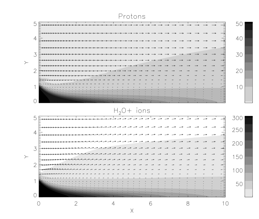
Figure 1: Density contours (shades of gray) and flow geometry (velocity vectors) for a model characterized by $Re^{a,b}=30$ and $\nu_{o}=0.1$ after 1500 simulation time units. The top panel shows the configuration for the proton plasma (species $a$) and the right side panel shows the “equilibrium” configuration for cometary H₂O+ ions. Density and velocity are in normalized units.

Figure 2: Velocity of H₂O+ ions in the tail of comet Swift-Tuttle as derived from the spectroscopic observations by Spinrad et al. (1994).

Figure 3: Comparison of the tailward velocity of H₂O+ ions in our numerical simulations (lines) and from the spectroscopic observations (symbols) of Spinrad et al. (1994) for models with different Reynolds number. The vertical dotted line indicates the position of the nucleus in the observations.

Figure 4: Comparison of the tailward velocity of H₂O+ ions in the numerical simulations (lines) and from the spectroscopic observations (symbols) of Spinrad et al. (1994) for models with different interspecies coupling parameter. The parameter $\nu_{o}$ is the ratio of the the flow crossing timescale $t_{\rm cross}=L/V_{o}$ to the timescale for coupling between species. The vertical dotted line indicates the position of the nucleus in the observations.

Figure 5: Comparison of the evolution of the tailward velocity of H₂O+ ions in our fiducial model ($Re^{a,b}=30$, $\nu_{o}=0.1$) in the numerical simulations (lines), and from the spectroscopic observations (symbols) of Spinrad et al. (1994).

References

- (1) Alfven, H. 1957, Tellus, 9, 92-96
- Baketal (86) Baker, D.N., Feldman, W.C., Gary, S.P., McComas, D.J., Middleditch, J. 1986, Geophys. Res. Lett., 13, 271
- (3) Biermann, L. 1951, Z. Astrophys., 29, 274-286
- (4) Biermann, L., Brosowski, B., Schmidt, H.U. 1967, Sol. Phys., 1, 254-283
- (5) Cravens, T.E., Gombosi, T.I. 2004, Adv.Sp.Res., 33, 1968
- Dobe (1999) Dobe, Z., Quest, K.B., Shapiro, V.D., Szego, K., Huba, J.D. 1999, Phys. Rev. Lett., 83, 260
- Goldsteinetal (1986) Goldstein, B.E. et al. 1986, in Proc. 20th ESLAB Symposium on the Exploration of Halley’s Comet, ESA SP-250, 229
- (8) Ip, W.-H. 2004, Adv.Sp.Res., 33, 605
- (9) Johnstone, A. et al. 1986, Nature, 321, 344
- Klimov (1986) Klimov, S. et al. 1986, Nature, 321, 292
- (11) Pérez-de-Tejada, H. 1989, J. Geophys. Res., 94, A10131
- (12) Pérez-de-Tejada, H. 1999, ApJ, 525,L65
- (13) Pérez-de-Tejada, H., Orozco, A., Dryer, M. 1980, Astrophys. Sp. Sci., 68, 233-243
- (14) Reme, H. 1991, in Cometary Plasma Processes, AGU monograph 61, ed. A.D. Johnstone (Washington, D.C.) 87
- Reyes-Ruiz (2009) Reyes-Ruiz, M., Perez-de-Tejada, H., Aceves, H., R. Vazquez, 2009, A&A submitted, arXiv:0812.1189 (RR09)
- Scarf (1986) Scarf, F.L., Ferdinand, V., Coroniti, V., Kennel, C.F., Gurnett, D.A., Ip, W.-H., Smith, E.J. 1986, Science, 232, 377
- (17) Shapiro, V.D., Szegö, K., Ride, S., Shevchenko, V. 1995, J. Geophys Res., 100, 21289
- (18) Spinrad, H., Brown, M.E., Jones, C.M. 1994, Astron.J, 108, 1462
- (19) Spreiter, J., Stahara, S. 1980, J. Geophys Res., 85, 7715
- (20) Szego, K. et al. 2000, Sp. Sci. Rev., 94,429
- Tsusmit (1986) Tsurutani, B.T., Smith, E.J. 1986, Geophys. Res. Lett., 13, 263
- (22) Wallis, M.K. 1973, Planet. Sp. Sci., 21, 1647