An equilibrium problem for the limiting eigenvalue distribution of rational Toeplitz matrices

Abstract

We consider the asymptotic behavior of the eigenvalues of Toeplitz matrices with rational symbol as the size of the matrix goes to infinity. Our main result is that the weak limit of the normalized eigenvalue counting measure is a particular component of the unique solution to a vector equilibrium problem. Moreover, we show that the other components describe the limiting behavior of certain generalized eigenvalues. In this way, we generalize the recent results of Duits and Kuijlaars [7] for banded Toeplitz matrices.

Keywords: Toeplitz matrix, rational function, generalized eigenvalues, (vector) potential theory.

1 Introduction

For an integrable function $f$ on the complex unit circle $\{z\mid|z|=1\}$ the Toeplitz matrix $T_{n}(f)$ of size $n\times n$ is defined by

$$T_{n}(f)=\begin{pmatrix}f_{i-j}\end{pmatrix}_{i,j=1}^{n}=\left(\begin{array}[]{lllll}f_{0}&f_{-1}&f_{-2}&f_{-3}&\ldots\\ f_{1}&f_{0}&f_{-1}&f_{-2}&\ldots\\ f_{2}&f_{1}&f_{0}&f_{-1}&\ldots\\ f_{3}&f_{2}&f_{1}&f_{0}&\ldots\\ \vdots&\vdots&\vdots&\vdots&\ddots\end{array}\right)_{n\times n},$$ (1.1)

where $f_{k}$ is the $k$th Fourier coefficient of $f$

$$f_{k}=\frac{1}{2\pi}\int_{0}^{2\pi}f({\rm e}^{{\rm i}t}){\rm e}^{-{\rm i}kt}dt.$$ (1.2)

The function $f$ is called the symbol of $T_{n}(f)$. In this paper we will be interested in symbols $f$ that are rational. That is, we assume that there exist polynomials $A$, $B_{1}$ and $B_{2}$ such that

$$f(z)=\frac{A(z)}{B_{1}(z)B_{2}(z)},$$ (1.3)

where the roots of $B_{1}$ (or $B_{2}$) lie inside (or outside) the unit circle. Thus we do not allow $f$ to have poles on the unit circle. We take $A$ so that it has no common roots with $B_{1}$ and $B_{2}$.

Note that if $B_{1}(z)=z^{q}$, $q\in\mathbb{N}$, and $B_{2}(z)\equiv 1$, then (1.3) reduces to the Laurent polynomial

$$f(z)=\frac{A(z)}{z^{q}}=\sum_{k=-q}^{p}f_{k}z^{k}$$ (1.4)

where

$$p=\deg A-q.$$

Thus we have $f_{k}=0$ for all $k>p$ and for all $k<-q$. The matrix $T_{n}(f)$ is then a banded Toeplitz matrix. The integers $p$ and $q$ in (1.4) correspond to the outermost non-zero diagonals in the lower and upper triangular part of this matrix, respectively. For a detailed discussion of banded Toeplitz matrices see [2].

We are interested in the asymptotic behavior of the eigenvalues of $T_{n}(f)$ as $n\to\infty$. It is known that the eigenvalues accumulate on a particular curve in the complex plane that we will introduce shortly. Moreover, there exists a measure on this curve describing the limiting distribution of the eigenvalues. It was shown in [7] that for banded Toeplitz matrices this limiting distribution is subject to an equilibrium problem that is naturally constructed out of the symbol. The purpose of the present paper is to extend this result to the case of rational symbols.

Let us first review some results on the asymptotic behavior of eigenvalues of rationally generated Toeplitz matrices. Let $f$ be as in (1.3) and $T_{n}(f)$ the associated Toeplitz matrix. Denote the spectrum of $T_{n}(f)$ as

$$\mathrm{sp}\ T_{n}(f)=\{\lambda\in\mathbb{C}\mid\det(T_{n}(f)-\lambda I)=0\}.$$

To describe the asymptotic behavior of the spectrum we introduce, as in [13], two different limiting sets

$$\liminf_{n\to\infty}\mathrm{sp}\ T_{n}(f)$$

consisting of all $\lambda\in\mathbb{C}$ for which there exists a sequence $\{\lambda_{n}\}_{n\in\mathbb{N}}$, with $\lambda_{n}\in\mathrm{sp}\ T_{n}(f)$ converging to $\lambda$, and the set

$$\limsup_{n\to\infty}\mathrm{sp}\ T_{n}(f)$$

consisting of all $\lambda$ for which there exists a sequence $\{\lambda_{n}\}_{n\in\mathbb{N}}$, with $\lambda_{n}\in\mathrm{sp}\ T_{n}(f)$ having a subsequence converging to $\lambda$.

It turns out that these limiting sets can be described in terms of solutions to the equation

$$0=f(z)-\lambda=\frac{A_{\lambda}(z)}{B_{1}(z)B_{2}(z)}$$ (1.5)

where

$$A_{\lambda}(z):=A(z)-\lambda B_{1}(z)B_{2}(z).$$ (1.6)

Following the analogy with (1.4), we define

$$q:=\deg B_{1},\qquad p:=\max(\deg A,\deg B_{1}\deg B_{2})-q.$$ (1.7)

To avoid trivial cases, in what follows we always assume that $p,q\geq 1$, see e.g. [6]. We also assume without loss of generality that

$$\textrm{gcd}\{k\mid f_{k}\neq 0\}=1,$$ (1.8)

see [2, Page 263].

Note that $A_{\lambda}(z)$ in (1.6) is a polynomial of degree $p+q$ in $z$, with each of its coefficients depending linearly on $\lambda$. There can be at most one value of $\lambda\in\mathbb{C}$ for which the leading coefficient vanishes. For all other $\lambda\in\mathbb{C}$, the polynomial $A_{\lambda}(z)$ has precisely $p+q$ roots $z=z(\lambda)$ (counting multiplicities) and we label them by absolute value as

$$0\leq|z_{1}(\lambda)|\leq|z_{2}(\lambda)|\leq\ldots\leq|z_{p+q}(\lambda)|.$$ (1.9)

In case where two or more subsequent roots in (1.9) have the same absolute value, we may arbitrarily label them so that (1.9) is satisfied. For the special value of $\lambda$ for which the polynomial $A_{\lambda}$ has less than $p+q$ roots, say $p+q-k$, we again order these roots $z_{1}(\lambda),\ldots,z_{p+q-k}(\lambda)$ as in (1.9) and then we set $z_{p+q-k+1}(\lambda)=\ldots=z_{p+q}(\lambda)=\infty$.

Define the curve

$$\Gamma_{0}:=\{\lambda\in\mathbb{C}\mid|z_{q}(\lambda)|=|z_{q+1}(\lambda)|\}.$$ (1.10)

The fact of the matter is that

$$\liminf_{n\to\infty}\mathrm{sp}\ T_{n}(f)=\limsup_{n\to\infty}\mathrm{sp}\ T_{n}(f)=\Gamma_{0}.$$ (1.11)

This result was first established by P. Schmidt and F. Spitzer [13] in the banded Toeplitz case (1.4), using a determinant identity by H. Widom [16]. The generalization to the case of rational symbols (1.3) is due to K.M. Day [6], based on an extension [5] of Widom’s determinant identity.

Let $\nu_{n}$ be the counting measure on the eigenvalues of $T_{n}(f)$

$$\nu_{n}=\frac{1}{n}\sum_{\lambda\in\mathrm{sp}\ T_{n}(f)}\delta_{\lambda}$$ (1.12)

where $\delta_{\lambda}$ is the Dirac measure at $\lambda$ and each eigenvalue is counted according to its multiplicity. It turns out that the measures $\nu_{n}$ converge weakly to a measure $\mu_{0}$ on $\Gamma_{0}$.

In the banded case (1.4) the measure $\mu_{0}$ is known to be absolutely continuous, and an explicit expression for this measure was given by I.I. Hirschman [8]. An alternative representation of $\mu_{0}$ can be obtained by setting $k=0$ in (1.14) below, cf. [7]. Further results about $\mu_{0}$ in the banded case can be found in [2, 7, 8, 15].

For Toeplitz matrices with rational symbol (1.3) the limiting eigenvalue measure does not need to be absolutely continuous. Indeed, it was shown by Day [6] that this measure has an absolutely continuous part together with at most two point masses.

Finally, we turn to the results of [7]. Consider the general system of curves

$$\Gamma_{k}=\{\lambda\in\mathbb{C}\mid|z_{q+k}(\lambda)|=|z_{q+k+1}(\lambda)|\},$$ (1.13)

for $k=-q+1,\ldots,p-1$. Each curve $\Gamma_{k}$ consists of finitely many analytic arcs. We equip every analytic arc of $\Gamma_{k}$ with an orientation and we define the $+$-side (or $-$-side) as the side on the left (or right) of the arc when traversing the arc according to its orientation.

For $k=-q+1,\ldots,p-1$ we define the measure

$$d\mu_{k}(\lambda)=\frac{1}{2\pi i}\sum_{j=1}^{q+k}\left(\frac{z_{j+}^{\prime}(\lambda)}{z_{j+}(\lambda)}-\frac{z_{j-}^{\prime}(\lambda)}{z_{j-}(\lambda)}\right)d\lambda$$ (1.14)

on the curve $\Gamma_{k}$. Here $d\lambda$ denotes the complex line element on each analytic arc of $\Gamma_{k}$, according to the chosen orientation of $\Gamma_{k}$. Moreover, $z_{j+}(\lambda)$ and $z_{j_{-}}(\lambda)$ are the boundary values of $z_{j}(\lambda)$ obtained from the $+$-side and $-$-side respectively of $\Gamma_{k}$. These boundary values exist except for a finite number of points. Note that (1.14) is actually independent of the choice of the orientation.

For the banded case it is shown in [7] that each $\mu_{k}$ is a finite positive measure. Moreover, $\mu_{0}$ is the measure of Hirschman, that is, the limit of the normalized eigenvalue counting measures $\nu_{n}$ as given in (1.12). The main observation in [7] is that the system of measures $\{\mu_{k}\}_{k}$ together uniquely minimizes an energy functional defined on the system of curves $\{\Gamma_{k}\}_{k}$.

The purpose of this paper is to prove that also for rational symbols the measures $\{\mu_{k}\}_{k}$ minimize an energy functional, thus generalizing the results in [7]. The general definition of the energy functional involves point sources that do not occur in the banded Toeplitz case. This is related to the phenomenon that the limiting eigenvalue distribution possibly has point masses for rationally generated Toeplitz matrices, as mentioned before. We also emphasize that the $\mu_{k}$ are absolutely continuous. It is to be understood that $\mu_{0}$ is the absolutely continuous part of the limiting eigenvalue distribution, with the possible point masses removed. Our results will be stated in detail in the next section.

2 Statement of results

2.1 Auxiliary definitions

First we introduce some definitions that will be used in the statement of our main theorems. For $k=0$ these definitions will be essentially the ones of Day [6], but we will state the definitions for general values of $k\in\{-q+1,\ldots,p-1\}$.

Definition 2.1.

Recall the notations (1.6)–(1.7). Define the coefficients $a_{k},b_{k}\in\mathbb{C}$, $k=-q,\ldots,p$, by

$$A_{\lambda}(z)=A(z)-\lambda B_{1}(z)B_{2}(z)=:\sum_{k=-q}^{p}(a_{k}-\lambda b_{k})z^{q+k}.$$ (2.1)

(Note the index shift.) Define $\lambda_{1},\lambda_{2}\in\overline{\mathbb{C}}:=\mathbb{C}\cup\{\infty\}$ such that

$$a_{-q}-b_{-q}\lambda_{1}=0,\qquad\textrm{and }a_{p}-b_{p}\lambda_{2}=0,$$

respectively. Define $k_{1},k_{2}\in\{1,\ldots,p+q\}$ to be the maximal indices for which

$$a_{k}-b_{k}\lambda_{1}=0,\qquad k=-q,\ldots,-q+k_{1}-1,$$

and

$$a_{k}-b_{k}\lambda_{2}=0,\qquad k=p-k_{2}+1,\ldots,p,$$

respectively. Here we make the convention that $a_{k}-b_{k}\lambda_{j}=0$ if $b_{k}=0$ and $\lambda_{j}=\infty$, $j=1,2$.

The numbers $\lambda_{1},\lambda_{2}$ in Definition 2.1 are the unique $\lambda$-values for which the polynomial $A_{\lambda}$ has some of its roots equal to $0$ (for $\lambda_{1}$) or to $\infty$ (for $\lambda_{2}$). In fact, the numbers $k_{1}$ and $k_{2}$ are chosen such that $A_{\lambda_{1}}$ has $k_{1}$ roots equal to zero, and $A_{\lambda_{2}}$ has $k_{2}$ roots at $\infty$. For all other values of $\lambda$, $A_{\lambda}$ has precisely $p+q$ roots (counting multiplicities) which are all non-zero and finite.

Remark 2.2.

By definition we have that $k_{1},k_{2}\leq p+q$. The case where $k_{1}>p+q$ or $k_{2}>p+q$ cannot occur since it would imply that all coefficients of $A_{\lambda}(z)$ are equal up to multiplication with a scalar. This would then imply that the numerator and denominator in (1.3) are equal up to a scalar factor, contrary to our assumptions. Note also that it is possible to have either $k_{1}=p+q$ or $k_{2}=p+q$, but not simultaneously. Indeed, in the latter case we would have that $A_{\lambda}(z)=(a_{-q}-\lambda b_{-q})+(a_{p}-\lambda b_{p})z^{p+q}$ and hence $B_{1}(z)B_{2}(z)=b_{-q}+b_{p}z^{p+q}$. The latter implies that either $p=0$ or $q=0$ which contradicts the assumption $p,q\geq 1$ made in the introduction.

Definition 2.3.

For each $k=-q+1,\ldots,p-1$ define

$$m_{1,k}=\max\left(1-\frac{q+k}{k_{1}},0\right)\in[0,1),$$ (2.2)

$$m_{2,k}=\max\left(1-\frac{p-k}{k_{2}},0\right)\in[0,1),$$ (2.3)

and

$$m_{k}=1-m_{1,k}-m_{2,k}.$$ (2.4)

The numbers $m_{1,k}$ and $m_{2,k}$ will be the weights of certain point masses, see further. The quantity $m_{k}$ will be the total mass of the measure $\mu_{k}$ in (1.14). Occasionally we will also consider $m_{1,k}$, $m_{2,k}$ and $m_{k}$ for the indices $k=-q$ or $k=p$.

Note that the $m_{k}$ are strictly positive for all $k$. Indeed, from the definition of $m_{1,k},m_{2,k},m_{k}$ and the fact that $k_{1}\leq p+q$ and $k_{2}\leq p+q$ it is easy to check that $m_{k}\geq 0$ for $k=-q+1,\ldots,p-1$. Moreover, if $m_{k}=0$ for some $k$ then $k_{1}=k_{2}=p+q$. However, in Remark 2.2 we observed that this is not possible.

Example 2.4.

Consider the banded case, i.e. $b_{0}=1$ and $b_{k}=0$ for all other $k$. In that case we have $\lambda_{1}=\lambda_{2}=\infty$, $k_{1}=q$ and $k_{2}=p$. Then the numbers $m_{1,k}$, $m_{2,k}$ and $m_{k}$ in Definition 2.3 are given in the following table

$$\left.\begin{array}[]{c|ccccccc}k&-q+1&\ldots&-1&0&1&\ldots&p-1\\ \hline\cr m_{1,k}&\frac{q-1}{q}&\ldots&\frac{1}{q}&0&0&\ldots&0\\ m_{2,k}&0&\ldots&0&0&\frac{1}{p}&\ldots&\frac{p-1}{p}\\ m_{k}&\frac{1}{q}&\ldots&\frac{q-1}{q}&1&\frac{p-1}{p}&\ldots&\frac{1}{p}\end{array}.\right.$$ (2.5)

The last row of (2.5) contains the masses of the measures $\mu_{k}$ appearing in [7].

Example 2.5.

Here are two examples of possible behavior when $q=4$ and $p=2$:

$$\left.\begin{array}[]{c|cccccc}k&-3&-2&-1&0&1\\ \hline\cr m_{1,k}&2/3&1/3&0&0&0\\ m_{2,k}&0&0&0&0&0\\ m_{k}&1/3&2/3&1&1&1\end{array},\right.\qquad\left.\begin{array}[]{c|ccccccc}k&-3&-2&-1&0&1\\ \hline\cr m_{1,k}&4/5&3/5&2/5&1/5&0\\ m_{2,k}&0&0&0&1/3&2/3\\ m_{k}&1/5&2/5&3/5&7/15&1/3\end{array},\right.$$ (2.6)

for the case where $(k_{1},k_{2})=(3,1)$ or $(5,3)$, respectively. This occurs e.g. for the rational symbols

$$\left\{\begin{array}[]{ll}f(z)=\frac{1+z^{2}+2z^{6}}{1+z^{2}+z^{3}+z^{5}+z^{6}}&\textrm{(left table),}\\ f(z)=\frac{1+z^{2}+z^{3}+2z^{5}+2z^{6}}{1+z^{2}+z^{3}+z^{5}+z^{6}}&\textrm{(right table).}\end{array}\right.$$

2.2 The equilibrium problem

Below we will consider measures $\mu$ supported on contours in $\mathbb{C}$. If the support is unbounded then we will assume that

$$\int\log(1+|x|)\ d\mu(x)<\infty.$$

For such a measure $\mu$ define its logarithmic energy as

$$I(\mu)=\int\int\ \log\frac{1}{|x-y|}\ d\mu(x)\ d\mu(y).$$ (2.7)

Similarly, for measures $\mu,\nu$ define their mutual energy as

$$I(\mu,\nu)=\int\int\ \log\frac{1}{|x-y|}\ d\mu(x)\ d\nu(y).$$ (2.8)

Definition 2.6.

(Compare with [7]) We call a vector of measures $\vec{\nu}=(\nu_{-q+1},\ldots,\nu_{p-1})$ admissible if $\nu_{k}$ has finite logarithmic energy, $\nu_{k}$ is supported on $\Gamma_{k}$, and $\nu_{k}$ has total mass $\nu_{k}(\Gamma_{k})=m_{k}$ for every $k=-q+1,\ldots,p-1$, recall (2.4).

The energy functional $J$ is defined by

$$J(\vec{\nu})=\sum_{k=-q+1}^{p-1}I(\nu_{k})-\sum_{k=-q+1}^{p-2}I(\nu_{k},\nu_{k+1})-\frac{\chi_{\lambda_{1}\neq\infty}\chi_{k_{1}<p+q}}{k_{1}}\int\log\frac{1}{|x-\lambda_{1}|}\ d\nu_{-q+k_{1}}(x)\\ -\frac{\chi_{\lambda_{2}\neq\infty}\chi_{k_{2}<p+q}}{k_{2}}\int\log\frac{1}{|x-\lambda_{2}|}\ d\nu_{p-k_{2}}(x).$$ (2.9)

Here we define $\chi_{\lambda_{1}\neq\infty}$ to be $1$ when $\lambda_{1}\neq\infty$ and $0$ otherwise. The quantities $\chi_{\lambda_{2}\neq\infty},\chi_{k_{1}<p+q}$ and $\chi_{k_{2}<p+q}$ are similarly defined.

The equilibrium problem is to minimize the energy functional (2.9) over all admissible vectors of positive measures $\vec{\nu}$.

The equilibrium problem may be understood intuitively as follows. On each of the curves $\Gamma_{k}$ one puts charged particles with total charge $m_{k}$. Particles that lie on the same curve repel each other. The particles on two consecutive curves attract each other, but with a strength that is only half as strong as the repulsion on a single curve. Particles on different curves that are non-consecutive do not interact with each other in a direct way. In addition, if $\lambda_{1}\neq\infty$ and $k_{1}<p+q$ then we have an external field acting on the particles on the curve $\Gamma_{-q+k_{1}}$. Similarly, if $\lambda_{2}\neq\infty$ and $k_{2}<p+q$ we have an external field acting on the particles on $\Gamma_{p-k_{2}}$. The external fields come from point charges at $\lambda=\lambda_{1}$ and $\lambda=\lambda_{2}$, respectively. The minus signs in (2.9) imply that these point charges are attractive. Such external fields are sometimes referred to as ‘sinks’. Note that there are no external fields acting on the other measures $\nu_{k}$, $k\not\in\{-q+k_{1},p-k_{2}\}$.

Note that the external fields acting on the measures $\nu_{-q+k_{1}}$ and $\nu_{p-k_{2}}$ do not occur in [7]. Indeed, in that case we have $\lambda_{1}=\lambda_{2}=\infty$ and hence $\chi_{\lambda_{1}\neq\infty}$ and $\chi_{\lambda_{2}\neq\infty}$ in (2.9) vanish, see Example 2.4.

For more information on equilibrium problems with external fields, see [10, 11, 12].

Remark 2.7.

In order for the above equilibrium problem to make sense, we need the energy functional $J$ in (2.9) to be bounded from below. A proof of this boundedness will be given in Lemma 3.7. For the boundedness it is important to note that

$$\lambda_{1}\not\in\Gamma_{-q+k_{1}}\textrm{ and }\lambda_{2}\not\in\Gamma_{p-k_{2}},$$ (2.10)

which follows immediately from the definitions of $k_{1}$ and $k_{2}$. Hence the sinks are not on the contours on which they are acting.

The following is our main theorem.

Theorem 2.8.

Recall the notations in (1.7), (1.9), (1.13) and (1.14) and assume that $p,q\geq 1$. Then

• The vector of measures $\vec{\mu}=(\mu_{k})_{k=-q+1}^{p-1}$ defined in (1.14) is admissible.

• For each $k\in\{-q+1,\ldots,p-1\}$ there exists a constant $l_{k}\in\mathbb{R}$ such that

  $$2\int\log\frac{1}{|\lambda-x|}\ d\mu_{k}(x)-\int\log\frac{1}{|\lambda-x|}\ d\mu_{k+1}(x)-\int\log\frac{1}{|\lambda-x|}\ d\mu_{k-1}(x)\\ -\frac{\chi_{\lambda_{1}\neq\infty}\chi_{k=-q+k_{1}}}{k_{1}}\log\frac{1}{|\lambda-\lambda_{1}|}-\frac{\chi_{\lambda_{2}\neq\infty}\chi_{k=p-k_{2}}}{k_{2}}\log\frac{1}{|\lambda-\lambda_{2}|}=l_{k},$$ (2.11)

  for $\lambda\in\Gamma_{k}\setminus\{\lambda_{1},\lambda_{2}\}$. Here we let $\mu_{-q}$ and $\mu_{p}$ be the zero measures.

• $\vec{\mu}=(\mu_{k})_{k=-q+1}^{p-1}$ is the unique solution to the equilibrium problem described above.

Theorem 2.8 will be proved in Section 3. Note that the equalities in Part (b) are precisely the Euler-Lagrange variational conditions of the equilibrium problem. Part (c) will then be a consequence of the convexity of the energy functional $J$ and the fact that $J$ is bounded from below.

2.3 The measures $\mu_{k}$ as limiting distributions of generalized eigenvalues

It was proved in [7] that in case of banded Toeplitz matrices, the measures $\mu_{k}$ for $k\neq 0$ also have an interpretation of being the limiting measures for certain generalized eigenvalues. For the rationally generated Toeplitz matrices such a result remains valid.

Definition 2.9.

For $k=-q+1,\ldots,p-1$ and $n\geq 1$ we define the polynomial ${P}_{k,n}$ by

$${P}_{k,n}(\lambda)=\det T_{n}(z^{-k}(f(z)-\lambda))$$

and we define the $k$th generalized spectrum of $T_{n}(f)$ by

$$\mathrm{sp}_{k}T_{n}(f)=\{\lambda\in\mathbb{C}\mid{P}_{k,n}(\lambda)=0\}.$$

Finally, we define $\mu_{k,n}$ as the normalized zero counting measure of $\mathrm{sp}_{k}T_{n}(f)$

$${\mu}_{k,n}=\frac{1}{n}\sum_{\lambda\in\mathrm{sp}_{k}T_{n}(f)}\delta_{\lambda},$$

where in the sum each $\lambda$ is counted according to its multiplicity as a zero of ${P}_{k,n}$.

The Toeplitz matrix $T_{n}(z^{-k}(f-\lambda))$ in Definition 2.9 may be interpreted as a shifted version of $T_{n}(f-\lambda)=T_{n}(f)-\lambda I$. For example if $k=2$ then by (1.2) we have

$$T_{n}(z^{-2}(f-\lambda))=\begin{pmatrix}f_{2}&f_{1}&f_{0}-\lambda&f_{-1}&f_{-2}&\ldots\\ f_{3}&f_{2}&f_{1}&f_{0}-\lambda&f_{-1}&\ldots\\ f_{4}&f_{3}&f_{2}&f_{1}&f_{0}-\lambda&\ldots\\ f_{5}&f_{4}&f_{3}&f_{2}&f_{1}&\ldots\\ f_{6}&f_{5}&f_{4}&f_{3}&f_{2}&\ldots\\ \vdots&\vdots&\vdots&\vdots&\vdots&\ddots\end{pmatrix}_{n\times n}.$$ (2.12)

We will show that for each $k$ the sequence $\{\mu_{k,n}\}_{n}$ has a limit. Moreover, the limiting measure will have point masses at $\lambda=\lambda_{1}$ (if $\lambda_{1}\neq\infty$) and $\lambda=\lambda_{2}$ (if $\lambda_{2}\neq\infty$) with weights at least $m_{1,k}$ and $m_{2,k}$, respectively. On the other hand, if $\lambda_{1}=\infty$ or $\lambda_{2}=\infty$ then the total mass of the limiting measure is reduced with at least $m_{1,k}$ or $m_{2,k}$ respectively. These facts can already be seen at the level of the finite-$n$ measures $\mu_{k,n}$ as the following proposition shows.

Proposition 2.10.

Let $k\in\{-q+1,\ldots,p-1\}$. Then the polynomial $P_{k,n}(\lambda)$ satisfies the following properties.

• $\left\{\begin{array}[]{ll}\textrm{$P_{k,n}(\lambda)$ is divisible by $(\lambda-\lambda_{1})^{m_{1,k}n-c}$,}&\textrm{if $\lambda_{1}\in\mathbb{C}$},\\ \textrm{$P_{k,n}(\lambda)$ has degree at most $(1-m_{1,k})n+c$,}&\textrm{if $\lambda_{1}=\infty$,}\end{array}\right.$

• $\left\{\begin{array}[]{ll}\textrm{$P_{k,n}(\lambda)$ is divisible by $(\lambda-\lambda_{2})^{m_{2,k}n-c}$,}&\textrm{if $\lambda_{2}\in\mathbb{C}$},\\ \textrm{$P_{k,n}(\lambda)$ has degree at most $(1-m_{2,k})n+c$,}&\textrm{if $\lambda_{2}=\infty$,}\end{array}\right.$

where $c\geq 0$ is a constant depending only on the symbol $f$.

Denote by $Q_{k,n}(\lambda)$ the quotient polynomial obtained from $P_{k,n}(\lambda)$ by removing all its factors $(\lambda-\lambda_{1})$ (if $\lambda_{1}\in\mathbb{C}$) and $(\lambda-\lambda_{2})$ (if $\lambda_{2}\in\mathbb{C}$). Then we have that

• $Q_{k,n}(\lambda)$ has degree at most $m_{k}n+2c$.

Proposition 2.10 will be proved in Section 4.1.

Since the measure (1.14) is absolutely continuous, the best one can hope for is $\mu_{k}$ being the absolutely continuous part of the limiting $k$th generalized eigenvalues distribution. This means that the possible point masses at $\lambda_{1}$ and $\lambda_{2}$ should be stripped out in $\mu_{k}$. This turns out to be indeed the case.

Theorem 2.11.

Let $k\in\{-q+1,\ldots,p-1\}$. Then

$$\liminf_{n\to\infty}\mathrm{sp}_{k}T_{n}(f)=\limsup_{n\to\infty}\mathrm{sp}_{k}T_{n}(f)=\Gamma_{k},$$

and

$$\lim_{n\to\infty}\int_{\mathbb{C}}\phi(\lambda)\ d\mu_{k,n}(\lambda)=\int_{\mathbb{C}}\phi(\lambda)\ d\mu_{k}(\lambda)+\chi_{\lambda_{1}\neq\infty}m_{1,k}\phi(\lambda_{1})+\chi_{\lambda_{2}\neq\infty}m_{2,k}\phi(\lambda_{2})$$ (2.13)

holds for every bounded continuous function $\phi$ on $\mathbb{C}$.

From (2.13) we see that $m_{1,k}$ and $m_{2,k}$ are the weights of the point masses at $\lambda_{1}$ and $\lambda_{2}$ in the limiting $k$th generalized eigenvalues distribution, if present.

2.4 Organization of the rest of the paper

The rest of this paper is organized as follows. Section 3 contains the proof of Theorem 2.8. In Section 4 we prove Proposition 2.10 and Theorem 2.11. Most of the proofs are inspired by the proofs given in [7] for the corresponding statements in the banded case, hence we will often refer to that paper. Finally, some illustrations of our results are given in Section 5.

3 Proof of Theorem 2.8

3.1 Proof of Theorem 2.8(a)–(b)

In this section we will prove Theorem 2.8(a)–(b). First we recall some elementary definitions and properties involving the algebraic equation $A_{\lambda}(z)=0$.

Definition 3.1.

([2, Section 11.2],[7]) A point $\lambda\in\mathbb{C}$ is called a branch point if $A_{\lambda}(z)=0$ has a multiple root. A point $\lambda\in\Gamma_{k}$ is an exceptional point of $\Gamma_{k}$ if $\lambda$ is a branch point, or if there is no open neighborhood $U$ of $\lambda$ such that $\Gamma_{k}\cap U$ is an analytic arc starting and terminating on $\partial U$.

Proposition 3.2.

Let $k\in\{-q+1,\ldots,p-1\}$. Then the set $\Gamma_{k}$ in (1.13) is the disjoint union of a finite number of open analytic arcs and a finite number of exceptional points. The set $\Gamma_{k}$ has no isolated points.

The proof of this proposition is similar as in [2, Theorem 11.9],[7],[13]. The condition (1.8) is needed to ensure that the $\Gamma_{k}$ are proper curves, i.e., they are 1-dimensional subsets of $\mathbb{C}$.

A major role is played by the functions $w_{k}$ which, for $k=-q+1,\ldots,p-1$ are defined by

$$w_{k}(\lambda)=\prod_{j=1}^{q+k}z_{j}(\lambda),\quad\lambda\in\mathbb{C}\setminus\Gamma_{k}.$$ (3.1)

The function $w_{k}$ is analytic in $\mathbb{C}\setminus\Gamma_{k}$. Occasionally we will also consider $w_{k}$ for the indices $k=-q$ or $k=p$.

Note that (1.14) may be written alternatively as

$$d\mu_{k}(\lambda)=\frac{1}{2\pi i}\left(\frac{w_{k+}^{\prime}(\lambda)}{w_{k+}(\lambda)}-\frac{w_{k-}^{\prime}(\lambda)}{w_{k-}(\lambda)}\right)d\lambda.$$

To discuss the integrability of this measure, we will need the asymptotic behavior of $\frac{w_{k}^{\prime}(\lambda)}{w_{k}(\lambda)}$. The relevant facts are listed in the following proposition.

Proposition 3.3.

Let $k\in\{-q+1,\ldots,p-1\}$ and recall the notations in Section 2.1. Then the following statements hold

1. For any $\lambda_{0}\in\overline{\mathbb{C}}\setminus\{\lambda_{1},\lambda_{2}\}$, there exists an $l\in\mathbb{N}:=\{1,2,3,\ldots\}$ such that

   $$\frac{w_{k}^{\prime}(\lambda)}{w_{k}(\lambda)}=\left\{\begin{array}[]{ll}O((\lambda-\lambda_{0})^{-1+1/l}),&\textrm{ if }\lambda_{0}\in\mathbb{C}\\ O(\lambda^{-1-1/l}),&\textrm{ if }\lambda_{0}=\infty\end{array}\right.$$

   as $\lambda\to\lambda_{0}$ with $\lambda\in\mathbb{C}\setminus\Gamma_{k}$. We have $l=1$ unless $\lambda_{0}$ is a branch point.

2. Assume $\lambda_{1}\neq\lambda_{2}$. Then near the point $\lambda_{1}$ there exists an $l\in\mathbb{N}$ such that

   $$\frac{w_{k}^{\prime}(\lambda)}{w_{k}(\lambda)}=\left\{\begin{array}[]{ll}\frac{1-m_{1,k}}{\lambda-\lambda_{1}}+O((\lambda-\lambda_{1})^{-1+1/l}),&\textrm{ if }\lambda_{1}\in\mathbb{C}\vspace{1mm}\\ -\frac{1-m_{1,k}}{\lambda}+O(\lambda^{-1-1/l}),&\textrm{ if }\lambda_{1}=\infty\end{array}\right.$$

   as $\lambda\to\lambda_{1}$ with $\lambda\in\mathbb{C}\setminus\Gamma_{k}$.

3. Assume $\lambda_{1}\neq\lambda_{2}$. Then near the point $\lambda_{2}$ there exists an $l\in\mathbb{N}$ such that

   $$\frac{w_{k}^{\prime}(\lambda)}{w_{k}(\lambda)}=\left\{\begin{array}[]{ll}\frac{-m_{2,k}}{\lambda-\lambda_{2}}+O((\lambda-\lambda_{2})^{-1+1/l}),&\textrm{ if }\lambda_{2}\in\mathbb{C}\vspace{1mm}\\ \frac{m_{2,k}}{\lambda}+O(\lambda^{-1-1/l}),&\textrm{ if }\lambda_{2}=\infty\end{array}\right.$$

   as $\lambda\to\lambda_{2}$ with $\lambda\in\mathbb{C}\setminus\Gamma_{k}$.

4. If $\lambda_{1}=\lambda_{2}$, then

   $$\frac{w_{k}^{\prime}(\lambda)}{w_{k}(\lambda)}=\left\{\begin{array}[]{ll}\frac{m_{k}}{\lambda-\lambda_{1}}+O((\lambda-\lambda_{1})^{-1+1/l}),&\textrm{ if }\lambda_{1}\in\mathbb{C}\vspace{1mm}\\ \frac{-m_{k}}{\lambda}+O(\lambda^{-1-1/l}),&\textrm{ if }\lambda_{1}=\infty\end{array}\right.$$

   as $\lambda\to\lambda_{1}=\lambda_{2}$ with $\lambda\in\mathbb{C}\setminus\Gamma_{k}$.

Proof.

First we make some general observations. For any $\lambda\in\overline{\mathbb{C}}\setminus\{\lambda_{1},\lambda_{2}\}$ the polynomial $A_{\lambda}(z)=0$ has roots $z_{j}(\lambda)$, $j=1,\ldots,p+q$, all of which are finite and non-zero (although some of the roots might occur with higher multiplicity). Zero roots or infinite roots can only occur if $\lambda\in\{\lambda_{1},\lambda_{2}\}$. As $\lambda\to\lambda_{1}$, then the $k_{1}$ smallest roots $z_{j}(\lambda)$ tend to zero like a power $(\lambda-\lambda_{1})^{1/k_{1}}$, while the other roots converge to non-zero constants. Similarly, as $\lambda\to\lambda_{2}$, then the $k_{2}$ largest roots $z_{j}(\lambda)$ tend to infinity like a power $(\lambda-\lambda_{2})^{-1/k_{2}}$, while the other roots converge to non-zero constants. These facts all follow from Definition 2.1.

To prove the first equality of Part (a), fix $\lambda_{0}\in\mathbb{C}\setminus\{\lambda_{1},\lambda_{2}\}$ and denote with $z_{j}=z_{j}(\lambda_{0})$, $j=1,\ldots,p+q$, the roots of $A_{\lambda_{0}}(z)$; by the discussion in the previous paragraph we have $z_{j}\in\mathbb{C}\setminus\{0\}$ for each $j$. Pick one of the roots $z_{j}$ which has the highest multiplicity $l$. Writing

$$A_{\lambda}(z)=(z-z_{j})^{l}P(z)+(\lambda-\lambda_{0})Q(z)$$

where $P(z)$ and $Q(z)$ are polynomials with $P(z_{j})\neq 0$ and $Q(z_{j})\neq 0$, it follows that

$$z_{j}(\lambda)=z_{j}+c(\lambda-\lambda_{0})^{1/l},\qquad\lambda\to\lambda_{0},$$

for some constant $c$. By taking the logarithmic derivative we obtain

$$\frac{z_{j}^{\prime}(\lambda)}{z_{j}(\lambda)}=O((\lambda-\lambda_{0})^{-1+1/l}),\qquad\lambda\to\lambda_{0}.$$

The first equality in Part (a) follows from this and the fact that

$$\frac{w_{k}^{\prime}(\lambda)}{w_{k}(\lambda)}=\sum_{j=1}^{q+k}\frac{z_{j}^{\prime}(\lambda)}{z_{j}(\lambda)}.$$

The second equality in Part (a) (for the case $\lambda_{0}=\infty$) is proved in a similar way, this time using a decomposition

$$A_{\lambda}(z)=(z-z_{j})^{l}\lambda P(z)+Q(z)$$

where again $P(z_{j})\neq 0$ and $Q(z_{j})\neq 0$.

To prove Part (b), first assume that $\lambda_{1}\neq\infty$. From the discussion in the first paragraph of this proof we obtain

$$\frac{z_{j}^{\prime}(\lambda)}{z_{j}(\lambda)}=\frac{1}{k_{1}(\lambda-\lambda_{1})}+O((\lambda-\lambda_{1})^{-1+1/k_{1}}),\quad\lambda\to\lambda_{1},$$

for all $j=1,\ldots,k_{1}$, while

$$\frac{z_{j}^{\prime}(\lambda)}{z_{j}(\lambda)}=O((\lambda-\lambda_{1})^{-1+1/l}),\quad\lambda\to\lambda_{1},$$

for $j=k_{1}+1,\ldots,p+q$ and a suitable $l\in\mathbb{N}$. Hence

$$\frac{w_{k}^{\prime}(\lambda)}{w_{k}(\lambda)} = \sum_{j=1}^{q+k}\frac{z_{j}^{\prime}(\lambda)}{z_{j}(\lambda)}$$

$$= \min\left(\frac{q+k}{k_{1}},1\right)\frac{1}{\lambda-\lambda_{1}}+O((\lambda-\lambda_{1})^{-1+1/\tilde{l}})$$

$$= \frac{1-m_{1,k}}{\lambda-\lambda_{1}}+O((\lambda-\lambda_{1})^{-1+1/\tilde{l}})$$

by virtue of (2.2), with $\tilde{l}=\max(l,k_{1})$. Similarly one can prove the case where $\lambda_{1}=\infty$. The proofs of Parts (c) and (d) are similar as well. ∎

Proposition 3.4.

For each $k$ we have that $\mu_{k}$ in (1.14) is a positive measure on $\Gamma_{k}$ with total mass $\mu_{k}(\Gamma_{k})=m_{k}$ as defined in (2.4).

Proof.

First we prove that the density (1.14) is locally integrable around the points $\lambda_{1}$, $\lambda_{2}$, $\infty$ (at least those of them which lie on the curve $\Gamma_{k}$). For $\infty$ this follows from the second equality in Proposition 3.3(a). For $\lambda_{1}$ this follows from Proposition 3.3(b) and taking into account that the $1/(\lambda-\lambda_{1})$ terms at the $+$-side and $-$-side in (1.14) cancel; a similar argument holds for the point $\lambda_{2}$.

The fact that the measure $\mu_{k}$ is positive follows from a Cauchy-Riemann argument as in [7, Proof of Proposition 4.1].

Finally, the statement that $\mu_{k}(\Gamma_{k})=m_{k}$ follows from a contour deformation argument as in [7, Proof of Proposition 4.1]. More precisely, we have

$$\mu_{k}(\Gamma_{k}) :=\frac{1}{2\pi i}\int_{\Gamma_{k}}\left(\frac{w_{k+}^{\prime}(\lambda)}{w_{k+}(\lambda)}-\frac{w_{k-}^{\prime}(\lambda)}{w_{k-}(\lambda)}\right)d\lambda$$

$$=\frac{1}{2\pi i}\int_{\mathcal{C}}\frac{w_{k}^{\prime}(\lambda)}{w_{k}(\lambda)}\ d\lambda+\chi_{\lambda_{1}\neq\infty}\mathrm{Res}\left(\frac{w_{k}^{\prime}(\lambda)}{w_{k}(\lambda)},\lambda=\lambda_{1}\right)+\chi_{\lambda_{2}\neq\infty}\mathrm{Res}\left(\frac{w_{k}^{\prime}(\lambda)}{w_{k}(\lambda)},\lambda=\lambda_{2}\right),$$ (3.2)

where $\mathcal{C}$ is a clockwise oriented contour surrounding $\Gamma_{k}$ and those points $\lambda_{1}$ and $\lambda_{2}$ which are finite, and where $\mathrm{Res}(h,\lambda)$ denotes the residue of $h$ at $\lambda$. Note that (3.2) is valid even when some of the $\lambda_{j}$ lie on the curve $\Gamma_{k}$, $j=1,2$, thanks to the local integrability of $\mu_{k}$ around these points. Applying the residue theorem once again, this time for the exterior domain of $\mathcal{C}$, we then find for the first term in (3.2) that

$$\frac{1}{2\pi i}\int_{\mathcal{C}}\frac{w_{k}^{\prime}(\lambda)}{w_{k}(\lambda)}\ d\lambda=-\mathrm{Res}\left(\frac{w_{k}^{\prime}(\lambda)}{w_{k}(\lambda)},\lambda=\infty\right).$$ (3.3)

The fact that $\mu_{k}(\Gamma_{k})=m_{k}$ then follows from (3.2)–(3.3) and the residue expressions in Proposition 3.3; recall also (2.4). ∎

Proposition 3.5.

For each $k$ we have that

$$\int\frac{1}{\lambda-x}\ d\mu_{k}(x)=-\frac{w_{k}^{\prime}(\lambda)}{w_{k}(\lambda)}+\chi_{\lambda_{1}\neq\infty}\frac{1-m_{1,k}}{\lambda-\lambda_{1}}+\chi_{\lambda_{2}\neq\infty}\frac{-m_{2,k}}{\lambda-\lambda_{2}},\quad\textrm{if }\lambda\in\mathbb{C}\setminus\Gamma_{k}$$ (3.4)

and

$$\int\log|\lambda-x|\ d\mu_{k}(x)=-\log|w_{k}(\lambda)|+\chi_{\lambda_{1}\neq\infty}(1-m_{1,k})\log|\lambda-\lambda_{1}|\\ -\chi_{\lambda_{2}\neq\infty}m_{2,k}\log|\lambda-\lambda_{2}|+\alpha_{k},\quad\textrm{if }\lambda\in\mathbb{C}$$ (3.5)

for a suitable constant $\alpha_{k}$.

Remark 3.6.

The quantities in the above proposition are only well-defined if $\lambda\neq\lambda_{j}$, $j=1,2$. However, one easily checks that $\lambda_{1}$ and $\lambda_{2}$ are removable singularities for the right hand sides of both (3.4) and (3.5), due to the continuity of the corresponding left hand sides.

Proof of Proposition 3.5.

The proof of (3.4) follows by contour deformation in a similar way as in the proof of Proposition 3.4. The relevant expression is now

$$\int_{\Gamma_{k}}\frac{1}{\lambda-x}\ d\mu_{k}(x):=\frac{1}{2\pi i}\int_{\Gamma_{k}}\frac{1}{\lambda-x}\left(\frac{w_{k+}^{\prime}(x)}{w_{k+}(x)}-\frac{w_{k-}^{\prime}(x)}{w_{k-}(x)}\right)dx=\frac{1}{2\pi i}\int_{\mathcal{C}}\frac{1}{\lambda-x}\frac{w_{k}^{\prime}(x)}{w_{k}(x)}\ dx\\ -\frac{w_{k}^{\prime}(\lambda)}{w_{k}(\lambda)}+\chi_{\lambda_{1}\neq\infty}\frac{1}{\lambda-\lambda_{1}}\mathrm{Res}\left(\frac{w_{k}^{\prime}(x)}{w_{k}(x)},x=\lambda_{1}\right)+\chi_{\lambda_{2}\neq\infty}\frac{1}{\lambda-\lambda_{2}}\mathrm{Res}\left(\frac{w_{k}^{\prime}(x)}{w_{k}(x)},x=\lambda_{2}\right),$$

where $\mathcal{C}$ is a clockwise oriented contour surrounding $\Gamma_{k}$, the point $\lambda$, and those points $\lambda_{1}$ and $\lambda_{2}$ which are finite. Now the integrand in the integral over $\mathcal{C}$ has zero residue at infinity and therefore this integral vanishes. Using the residue expressions in Proposition 3.3 one then arrives at the right hand side of (3.4). Finally, the proof of (3.5) then follows by integrating (3.4), see also [7]. ∎

Now we are ready to prove Theorem 2.8(a)–(b).

Proof of Theorem 2.8(a).

Taking into account Proposition 3.4, it suffices to show that the logarithmic energy $I(\mu_{k})$ is bounded for each $k\in\{-q+1,\ldots,p-1\}$. The latter follows by integrating (3.5) over $\mu_{k}(\lambda)$. Then the left hand side becomes $-I(\mu_{k})$, so it suffices to show that each of the four terms in the right hand side is bounded. For the fourth term this is evident since $\mu_{k}$ has finite mass. For the two middle terms this follows from our earlier observation that $\mu_{k}$ is integrable around $\lambda_{1}$ and $\lambda_{2}$ (assuming they are on the curve $\Gamma_{k}$), which is still true when multiplying with the logarithmic singularities $\log|\lambda-\lambda_{1}|$ and $\log|\lambda-\lambda_{2}|$. A similar argument holds for the first term. ∎

Proof of Theorem 2.8(b).

The proof of Part (b) follows from (3.5) and the auxiliary results

$$-\log|w_{k+1}(\lambda)|+2\log|w_{k}(\lambda)|-\log|w_{k-1}(\lambda)|=\log\left|\frac{\prod_{j=1}^{k}z_{j}(\lambda)^{2}}{\prod_{j=1}^{k+1}z_{j}(\lambda)\prod_{j=1}^{k-1}z_{j}(\lambda)}\right|=\log\left|\frac{z_{k}(\lambda)}{z_{k+1}(\lambda)}\right|=0$$

for $\lambda\in\Gamma_{k}\setminus\{\lambda_{1},\lambda_{2}\}$, and

$$-m_{1,k+1}+2m_{1,k}-m_{1,k-1}=\left\{\begin{array}[]{ll}-1/k_{1}&k=-q+k_{1}\\ 0&k\in\{-q+1,\ldots,p-1\}\setminus\{-q+k_{1}\}\end{array},\right.$$ (3.6)

$$-m_{2,k+1}+2m_{2,k}-m_{2,k-1}=\left\{\begin{array}[]{ll}-1/k_{2}&k=p-k_{2}\\ 0&k\in\{-q+1,\ldots,p-1\}\setminus\{p-k_{2}\}\end{array}.\right.$$ (3.7)

Here the boundary terms $m_{1,k}$, $m_{2,k}$ for $k=-q$ or $k=p$ are defined by the usual formulae (2.2)–(2.3). These considerations imply the desired result for $\lambda\in\Gamma_{k}\setminus\{\lambda_{1},\lambda_{2}\}$; the cases $\lambda=\lambda_{1}$ and $\lambda=\lambda_{2}$ then follow by continuity. ∎

3.2 Proof of Theorem 2.8(c)

To prove Theorem 2.8(c) we rewrite (2.9) in the following way, compare with [7, Eq. (2.12)]:

$$J(\vec{\nu})=\left(\sum_{k=-q+1}^{p-2}\frac{m_{k}m_{k+1}}{2}I\left(\frac{\nu_{k}}{m_{k}}-\frac{\nu_{k+1}}{m_{k+1}}\right)\right)+\frac{1}{2k_{1}m_{k_{1}}}I(\nu_{-q+k_{1}})+\frac{1}{2k_{2}m_{k_{2}}}I(\nu_{p-k_{2}})\\ -\frac{\chi_{\lambda_{1}\neq\infty}}{k_{1}}\int\log\frac{1}{|x-\lambda_{1}|}\ d\nu_{-q+k_{1}}(x)-\frac{\chi_{\lambda_{2}\neq\infty}}{k_{2}}\int\log\frac{1}{|x-\lambda_{2}|}\ d\nu_{p-k_{2}}(x).$$ (3.8)

We leave it to the reader to check the correctness of this identity; note that the calculation makes use of the auxiliary result

$$-m_{k+1}+2m_{k}-m_{k-1}=\left\{\begin{array}[]{ll}1/k_{1}&k=-q+k_{1}\neq p-k_{2}\\ 1/k_{2}&k=p-k_{2}\neq-q+k_{1}\\ 1/k_{1}+1/k_{2}&k=-q+k_{1}=p-k_{2}\\ 0&k\in\{-q+1,\ldots,p-1\}\setminus\{-q+k_{1},p-k_{2}\}\end{array}\right.$$

for $k\in\{-q+1,\ldots,p-1\}$, which follows from (2.4) and (3.6)–(3.7). Here we recall the boundary values $m_{-q}=m_{p}=0$.

We also invoke the fact that

$$I(\nu_{1}-\nu_{2})\geq 0,$$ (3.9)

whenever $\nu_{1}$ and $\nu_{2}$ are positive measures with $\nu_{1}(\mathbb{C})=\nu_{2}(\mathbb{C})\leq\infty$. This is a well-known result if $\nu_{1}$ and $\nu_{2}$ have bounded support [12]. If the support is unbounded this is a recent result of Simeonov [14].

Lemma 3.7.

The energy functional (2.9) is bounded from below on the set of admissible vectors of measures $\vec{\nu}$.

Proof.

From (3.8)–(3.9) we see that in order to show that the energy functional $J(\vec{\nu})$ is bounded from below, it is sufficient to show that

$$\frac{1}{2k_{1}m_{k_{1}}}I(\nu_{-q+k_{1}})-\frac{\chi_{\lambda_{1}\neq\infty}}{k_{1}}\int\log\frac{1}{|x-\lambda_{1}|}\ d\nu_{-q+k_{1}}(x)$$ (3.10)

and

$$\frac{1}{2k_{2}m_{k_{2}}}I(\nu_{p-k_{2}})-\frac{\chi_{\lambda_{2}\neq\infty}}{k_{2}}\int\log\frac{1}{|x-\lambda_{2}|}\ d\nu_{p-k_{2}}(x)$$

are both bounded from below on the set of admissible vectors of measures $\vec{\nu}$. Let us check this for the first term (3.10). We will use that

$$\lambda_{1}\not\in\Gamma_{-q+k_{1}},$$

a fact already observed in (2.10), which follows immediately from the definition of $k_{1}$. Now we distinguish between two cases. The first case is when $\lambda_{1}=\infty$. Then the second term in (3.10) drops out while on the other hand $\infty=\lambda_{1}\not\in\Gamma_{-q+k_{1}}$, so the contour $\Gamma_{-q+k_{1}}$ is bounded and therefore the first term in (3.10) is bounded from below as well.

The second case is when $\lambda_{1}\neq\infty$. Then standard arguments from potential theory show that the expression (3.10) is minimized precisely when $\nu_{-q+k_{1}}$ is the balayage of the Dirac point mass at $\lambda_{1}$ onto the curve $\Gamma_{-q+k_{1}}$, and in particular this expression is bounded from below [12, Chapter 2]. ∎

Remark 3.8.

The above proof goes through because the constant factor in front of the first term in (3.10) is precisely $1/2$. If this constant factor is different from $1/2$ then the connection with balayage measures breaks down, and in fact if the constant is larger than $1/2$ then the energy functional is not bounded from below anymore.

Proof of Theorem 2.8(c).

Assume that $\vec{\mu}$ is a vector of admissible measures satisfying the equalities in Theorem 2.8(b), and let $\vec{\nu}$ be any admissible vector of measures. We need to prove that $J(\vec{\nu})\geq J(\vec{\mu})$ with equality if and only if $\vec{\nu}=\vec{\mu}$. Note that the equalities in Theorem 2.8(b) are precisely the Euler-Lagrange variational conditions of the equilibrium problem. The result then follows from the fact that the energy functional $J$ is convex and bounded from below. More precisely, one can use exactly the same argument as in [7, Proofs of Lemma 2.3 and Theorem 2.3(c)], taking into account (3.8)–(3.9). There are some modifications induced by the external fields, but this does not lead to problems since the latter act in a linear way on the measures. ∎

4 Proofs of Proposition 2.10 and Theorem 2.11

4.1 Proof of Proposition 2.10

The proof of Proposition 2.10 is based on the reduction of a rationally generated Toeplitz matrix into banded form, which will then allow us to follow the proof in [7, Proof of Prop. 2.5]. Let us recall from (1.5) that

$$f(z)-\lambda=\frac{A_{\lambda}(z)}{B_{1}(z)B_{2}(z)},$$

where the numerator $A_{\lambda}(z)$ is a polynomial in $z$. Then we claim that for any $k\in\{-q+1,\ldots,p-1\}$ and for any $n$ sufficiently large, the rationally generated Toeplitz matrix with symbol $z^{-k}(f(z)-\lambda)$ can be reduced into banded form by the factorization

$$L_{n}T_{n}\left(z^{-k}(f(z)-\lambda)\right)R_{n}=T_{n}\left(z^{-q-k}A_{\lambda}(z)\right)+\begin{pmatrix}C&0\\ 0&0\end{pmatrix}_{n\times n},$$ (4.1)

where

$$L_{n}=T_{n}(B_{2}(z)),\qquad R_{n}:=T_{n}\left(z^{-q}B_{1}(z)\right),$$

are non-singular lower and upper triangular Toeplitz matrices respectively. The middle factor in the left hand side of (4.1) is our rationally generated Toeplitz matrix of interest, and (4.1) shows that it can be reduced to the banded matrix pencil in the right hand side. Here $C$ is a matrix whose size and entries are independent of $n$ but depend only on the symbol $f(z)$. For more information on factorizations of the type (4.1) see e.g. [4, Prop. 2.12] and also [5, 9].

From (4.1) we immediately deduce that

$$P_{k,n}(\lambda) := \det T_{n}\left(z^{-k}(f(z)-\lambda)\right)$$ (4.2)

$$= \frac{1}{\kappa}\det\left(T_{n}\left(z^{-q-k}A_{\lambda}(z)\right)+\begin{pmatrix}C&0\\ 0&0\end{pmatrix}_{n\times n}\right),$$

where $\kappa\neq 0$ is a numerical constant, given by the product of the diagonal entries of the two triangular factors $L_{n}$ and $R_{n}$ in (4.1).

We are now ready for the proof of Proposition 2.10. The proof will follow by expanding the determinant in (4.2) by a basic combinatorial argument, see also [7, Proof of Prop. 2.5].

Proof of Proposition 2.10(a).

The proposition is obvious if $m_{1,k}=0$. So we will assume below that $m_{1,k}>0$, or equivalently

$$q+k<k_{1}.$$ (4.3)

First we consider the case where $\lambda_{1}\neq\infty$. By expanding the determinant in (4.2) we find

$$P_{k,n}(\lambda)=\frac{1}{\kappa}\sum_{\pi\in S_{n}}\prod_{j=1}^{n}\left(a_{j-\pi(j)+k}-\lambda b_{j-\pi(j)+k}+\chi_{j\leq|C|}\chi_{\pi(j)\leq|C|}\ c_{j,\pi(j)}\right).$$

Here $S_{n}$ denotes the set of all permutations of $\{1,\ldots,n\}$, and we denote with $|C|$ the maximum of the row and column sizes of the matrix $C$; note that this number is independent of $n$. By the band structure it follows that we only have non-zero contributions for the permutations $\pi$ that satisfy

$$-q-k\leq j-\pi(j)\leq p-k\qquad\textrm{for all $j=|C|+1,\ldots,n$}.$$ (4.4)

Denote, for $\pi\in S_{n}$,

$$N_{\pi}=\{j\mid j-\pi(j)\in\{-q-k,\ldots,-q-k+k_{1}-1\}\}.$$ (4.5)

The set $N_{\pi}$ contains all indices $j$ for which the $(j,\pi(j))$ entry lies in the union of the $k_{1}$ topmost bands of the banded matrix in (4.2). By assumption (4.3) these bands include the main diagonal $j-\pi(j)=0$ and by definition of $k_{1}$ we have that the entries in these bands are all divisible by $(\lambda-\lambda_{1})$.

Denote the number of elements of $N_{\pi}$ in (4.5) by $|N_{\pi}|$. Then obviously

$$P_{k,n}\textrm{ is divisible by }(\lambda-\lambda_{1})^{\min_{\pi\in S_{n}}|N_{\pi}|},$$ (4.6)

where we minimize over all permutations $\pi\in S_{n}$ satisfying (4.4).

Let $\pi\in S_{n}$ satisfy (4.4). We give a lower bound for $|N_{\pi}|$. Since $\sum_{j=1}^{n}(j-\pi(j))=0$ we obtain

$$\sum_{j=1}^{n}(j-\pi(j))_{+}=\sum_{j=1}^{n}(\pi(j)-j)_{+},$$ (4.7)

where $(\cdot)_{+}$ is defined as $(a)_{+}=\max(0,a)$ for $a\in\mathbb{R}$. From the above definitions we also have that

$$\left\{\begin{array}[]{ll}j-\pi(j)\geq-q-k,&\textrm{ if }j\in N_{\pi}\\ j-\pi(j)\geq-q-k+k_{1},&\textrm{ if }j\in\{|C|+1,\ldots,n\}\setminus N_{\pi}.\end{array}\right.$$ (4.8)

By combining (4.7) and (4.8) we find that

$$(-q-k+k_{1})(n-|N_{\pi}|)+\tilde{c}\leq\sum_{j=1}^{n}(j-\pi(j))_{+}=\sum_{j=1}^{n}(\pi(j)-j)_{+}\leq(q+k)|N_{\pi}|-\tilde{c}.$$

Here $\tilde{c}\geq 0$ is a correction term which is due to the presence of the matrix $C$ in the top left matrix corner in (4.2); the number $\tilde{c}$ is clearly bounded from above. We then obtain

$$|N_{\pi}|\geq\frac{k_{1}-q-k}{k_{1}}n-c=\left(1-\frac{q+k}{k_{1}}\right)n-c=m_{1,k}n-c,$$ (4.9)

where we used (2.2) and (4.3), and where we put $c:=2\tilde{c}/k_{1}$. The first statement in Proposition 2.10(a) now follows from (4.6) and (4.9).

The proof of the second statement in Proposition 2.10(a) (for $\lambda_{1}=\infty$) is similar to the one above. Now one uses that all the entries $a_{j-\pi(j)+k}-\lambda b_{j-\pi(j)+k}$ in the bands indexed by $j\in N_{\pi}$ have their $\lambda$-coefficient $b_{j-\pi(j)+k}=0$, which then yields in a similar way to (4.6) and (4.9) that

$$\deg P_{k,n}\leq n-\min_{\pi\in S_{n}}|N_{\pi}|\leq(1-m_{1,k})n+c,$$ (4.10)

as desired. ∎

Proof of Proposition 2.10(b).

Similar to Part (a). ∎

Proof of Proposition 2.10(c).

Part (c) follows immediately from Parts (a) and (b), together with (2.4), in case where $\lambda_{1}\neq\lambda_{2}$. The case where $\lambda_{1}=\lambda_{2}$ can be obtained as well, by observing that at least one of the numbers $m_{1,k}$ and $m_{2,k}$ must be zero in that case. The latter follows since otherwise the numerator and denominator in (1.3) are equal up to multiplication with a scalar, contrary to our assumptions. ∎

4.2 Proof of Theorem 2.11

To prove Theorem 2.11 we need to manipulate the polynomial $P_{k,n}(\lambda)$. To this end we will use a determinant identity by K.M. Day which we state next.

To state the identity, we need some notations. Denote with $\beta_{i}$ and $\gamma_{i}$ the zeros of $B_{1}(z)$ and $B_{2}(z)$, respectively. Recall the notation $z_{i}=z_{i}(\lambda)$ for the roots of $A_{\lambda}(z)$. Thus

$$A_{\lambda}(z) = c\prod_{i=1}^{p+q}(z-z_{i}(\lambda))$$ (4.11)

$$B_{1}(z) = c_{1}\prod_{i=1}^{q}(z-\beta_{i})$$ (4.12)

$$B_{2}(z) = c_{2}\prod_{i=1}^{\deg B_{2}(z)}(z-\gamma_{i}),$$ (4.13)

where $c$, $c_{1}$, $c_{2}$ are non-zero constants.

The following theorem was proved under some additional hypotheses by K.M. Day [5]. Other proofs are in [3, 9], the former of them stated under the weakest assumptions. We state the theorem in the form that is most convenient for our purposes.

Theorem 4.1.

(Day’s determinant identity). Let $k\in\{-q+1,\ldots,p-1\}$ and let $\lambda\in\mathbb{C}\setminus\{\lambda_{1},\lambda_{2}\}$ be such that all roots of $A_{\lambda}(z)$ are distinct. Then

$$P_{k,n}(\lambda)=\det T_{n}(z^{-k}(f-\lambda))=\sum_{S}C_{S}(\lambda)(w_{S}(\lambda))^{n},$$ (4.14)

where the sum is over all subsets $S\subset\{1,2,\ldots,p+q\}$ of cardinality $|S|=q+k$ and for each such $S$ we have

$$w_{S}(\lambda):=(-1)^{q+k}(a_{-q}-b_{-q}\lambda)\left(\prod_{j\in S}z_{j}(\lambda)\right)^{-1}$$ (4.15)

and (with $\overline{S}:=\{1,2,\ldots,p+q\}\setminus S$)

$$C_{S}(\lambda):=\prod_{j\in\overline{S}}z_{j}(\lambda)^{k}\prod_{\small{\begin{array}[]{l}i\in S,r\in R,\\ j\in\bar{S},t\in T\end{array}}}\frac{(z_{j}(\lambda)-\beta_{r})(\gamma_{t}-z_{i}(\lambda))}{(z_{j}(\lambda)-z_{i}(\lambda))(\gamma_{t}-\beta_{r})},$$

with $R=\{1,\ldots,q\}$ and $T:=\{1,\ldots,\deg B_{2}(z)\}$.

Incidentally, observe that (4.15) can be written alternatively as

$$w_{S}(\lambda)=(-1)^{p-k}(a_{p}-b_{p}\lambda)\prod_{j\in\overline{S}}z_{j}(\lambda).$$ (4.16)

We note that in case where $k\in\{0,\ldots,p-1\}$, our formulation of Theorem 4.1 follows directly from the one of [5]; for the case $k\in\{-q+1,\ldots,-1\}$ it can be obtained from the result of [5] by working with the transposed matrix.

From (4.14)–(4.15) we see that for large $n$, the main contribution in (4.14) comes from those subsets $S$ for which $|w_{S}(\lambda)|$ is the largest possible. For $\lambda\in\mathbb{C}\setminus\Gamma_{k}$ there is a unique such $S$, namely

$$S=S_{k}:=\{1,2,\ldots,q+k\}.$$

Now we are ready to show that the asymptotic distribution of the $k$th generalized eigenvalues of $T_{n}(f)$ is described by the measure $\mu_{k}$, together with possible point masses at $\lambda_{1}$ and $\lambda_{2}$. First we prove this at the level of the Cauchy transforms.

Proposition 4.2.

Let $k\in\{-q+1,\ldots,p-1\}$. Then

$$\lim_{n\to\infty}\int_{\mathbb{C}}\frac{d\mu_{k,n}(x)}{\lambda-x}=\int_{\mathbb{C}}\frac{d\mu_{k}(x)}{\lambda-x}+\chi_{\lambda_{1}\neq\infty}\frac{m_{1,k}}{\lambda-\lambda_{1}}+\chi_{\lambda_{2}\neq\infty}\frac{m_{2,k}}{\lambda-\lambda_{2}}$$ (4.17)

uniformly on compact subsets of $\mathbb{C}\setminus\Gamma_{k}$.

Remark 4.3.

The above proposition implicitly assumes that $\lambda\neq\lambda_{j}$, $j=1,2$. However one checks that if $\lambda_{j}\in\mathbb{C}\setminus\Gamma_{k}$ then $\lambda_{j}$ is a removable singularity for the right hand side of (4.17), due to the continuity of the left hand side, and then the uniform convergence still applies.

Proof of Proposition 4.2.

As already mentioned, for large $n$ the dominant term in Day’s determinant identity Theorem 4.1 is obtained by taking $S=S_{k}:=\{1,2,\ldots,q+k\}$. Then we find in the same way as in [7, Proof of Corollary 5.3] that

$$\lim_{n\to\infty}\int_{\mathbb{C}}\frac{d\mu_{k,n}(x)}{\lambda-x}=\lim_{n\to\infty}\frac{1}{n}\sum_{\lambda_{i}\in\textrm{sp}_{k}\ T_{n}(f)}\frac{1}{\lambda-\lambda_{i}}=\lim_{n\to\infty}\frac{1}{n}\frac{P^{\prime}_{k,n}(\lambda)}{P_{k,n}(\lambda)}\\ =\frac{w_{S_{k}}^{\prime}(\lambda)}{w_{S_{k}}(\lambda)}=-\frac{w_{k}^{\prime}(\lambda)}{w_{k}(\lambda)}+\chi_{\lambda_{1}\neq\infty}\frac{1}{\lambda-\lambda_{1}}$$ (4.18)

uniformly on compact subsets of $\mathbb{C}\setminus\Gamma_{k}$, where the last transition of (4.18) follows from (3.1) and (4.15). Now from Proposition 3.5 we see that the right hand side of (4.18) equals the right hand side of (4.17). The proposition is proved. ∎

Now we are ready for the

Proof of Theorem 2.11.

From the convergence of the Cauchy transforms in Proposition 4.2 we deduce that

$$\mu_{k,n}\ \to\ \mu_{k}+m_{1,k}\chi_{\lambda_{1}\neq\infty}\delta_{\lambda_{1}}+m_{2,k}\chi_{\lambda_{2}\neq\infty}\delta_{\lambda_{2}}$$

in the weak-star sense, which means that (2.13) holds for every continuous $\phi$ that vanishes at infinity. Now a priori, it is not immediate that (2.13) holds for all bounded continuous functions since it is possible that $\mu_{k,n}$ has mass leaking to infinity as $n\to\infty$. However, from Proposition 2.10 it follows that this cannot happen, i.e., the measures $\{\mu_{k,n}\}_{n}$ are tight. Thus (2.13) holds indeed for all bounded continuous functions. For more details see [7, Proof of Theorem 2.6]. ∎

5 Example

Consider the rationally generated Toeplitz matrix with symbol

$$f(z)=\frac{1}{2z^{2}-5z+2}=\frac{1}{(2z-1)(z-2)}$$ (5.1)

defined on the complex unit circle. We may compute the Fourier series of this symbol explicitly and find

$$f(z)=\ldots-\frac{1}{12z^{3}}-\frac{1}{6z^{2}}-\frac{1}{3z}-\frac{1}{6}-\frac{z}{12}-\frac{z^{2}}{24}-\frac{z^{3}}{48}\ldots.$$

So the rationally generated Toeplitz matrix $T_{n}(f)$ looks like

$$T_{n}(f)=-\begin{pmatrix}1/6&1/3&1/6&1/12&\ldots\\ 1/12&1/6&1/3&1/6&\ldots\\ 1/24&1/12&1/6&1/3&\ldots\\ 1/48&1/24&1/12&1/6&\ldots\\ \vdots&\vdots&\vdots&\vdots&\ddots\end{pmatrix}_{n\times n}.$$

Equation (1.6) now becomes

$$A_{\lambda}(z)=1-\lambda(2z^{2}-5z+2),$$

and (1.7) leads to $p=q=1$. The roots of $A_{\lambda}(z)$ are given by

$$z_{1,2}(\lambda)=\frac{1}{4\lambda}(5\lambda\pm\sqrt{9\lambda^{2}+8\lambda}),$$

and they should be labeled in such a way that $|z_{1}(\lambda)|\leq|z_{2}(\lambda)|$ for all $\lambda$. The roots $z_{1}(\lambda)$ and $z_{2}(\lambda)$ are coalescing precisely when $9\lambda^{2}+8\lambda=0$, so the branch points are $\lambda=0$ and $\lambda=-8/9$.

Since $p=q=1$, there is only one relevant index $k$ in (1.13), namely $k=0$. The corresponding set $\Gamma_{0}$ is simply the line segment connecting the branch points $\lambda=0$ and $\lambda=-8/9$:

$$\Gamma_{0}=\{\lambda\in\mathbb{C}\mid|z_{1}(\lambda)|=|z_{2}(\lambda)|\}=[-8/9,0].$$

This may be checked from a straightforward calculation.

Definitions 2.1 and 2.3 now specialize as follows: $\lambda_{1}=1/2$, $\lambda_{2}=0$, $k_{1}=1$, $k_{2}=2$, and $m_{1,0}=0$, $m_{2,0}=1/2$ and $m_{0}=1/2$. Thus the limiting eigenvalue distribution of the matrix $T_{n}(f)$ for $n\to\infty$ consists of an absolutely continuous part $\mu_{0}$ with total mass $1/2$, supported on $\Gamma_{0}=[-8/9,0]$, and a singular part which is a point mass of mass $1/2$ at $\lambda=0$.

The energy functional (2.9) now specializes to

$$I(\nu_{0})-\int\log\frac{1}{|x-1/2|}\ d\nu_{0}(x).$$ (5.2)

So $\mu_{0}$ is the minimizer of (5.2) over all measures $\nu_{0}$ on $\Gamma_{0}=[-8/9,0]$ with total mass $1/2$. The second term in (5.2) can be interpreted as an attraction of $\mu_{0}$ towards the point $\lambda=1/2$.

The measure $\mu_{0}$ is absolutely continuous with density given by (1.14) (with $k=0$ and $p=q=1$). The density can be explicitly computed, but we will omit the result since it does not lead to considerable insight. We only mention that the density blows up like an inverse square root near both endpoints $\lambda=0$ and $\lambda=-8/9$. More precisely, it behaves approximately like $0.28/\sqrt{|\lambda|}$ near $\lambda=0$ and like $0.10/\sqrt{\lambda+8/9}$ near $\lambda=-8/9$.

Figure 1 contains a plot of the limiting density. The figure shows that there is more mass near $0$ than near $-8/9$, which is due to the attraction towards $\lambda=1/2$ in (5.2).

Figure 2 shows the result of a numerical computation of the eigenvalues of $T_{n}(f)$ with $n=60$. Note that approximately half of the eigenvalues is located at zero, according to Proposition 2.10; in fact we have $c=0$ in this case.

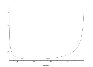
Figure 1: Density of the measure $\mu_{0}$ on $\Gamma_{0}=[-8/9,0]$ for the symbol (5.1). The density blows up like a square root near both endpoints $-8/9$ and $0$. There is more mass near $0$ due to the attraction towards $\lambda=1/2$.

Figure 2: Eigenvalues of the matrix $T_{n}(f)$ for the symbol (5.1), computed numerically in Maple for $n=60$ using high precision arithmetic. All the eigenvalues are real. There are $30$ of them in the open interval $(-8/9,0)$, together with a $30$-fold eigenvalue at $\lambda=0$.

We may consider the following modification of (5.1),

$$f(z)=\frac{1+\epsilon z}{2z^{2}-5z+2}=\frac{1+\epsilon z}{(2z-1)(z-2)},$$ (5.3)

where $\epsilon>0$ is some small number. It is still true that $\lambda_{1}=1/2$ and $\lambda_{2}=0$ for any $\epsilon$, but for $\epsilon$ non-zero we now have $k_{1}=k_{2}=1$, $m_{1,0}=m_{2,0}=0$ and $m_{0}=1$. Thus the limiting eigenvalue distribution of $T_{n}(f)$ is absolutely continuous (without point mass), it has total mass $1$, and it is supported on the interval $\Gamma_{0}$ joining the two branch points

$$\frac{-4-5\epsilon\pm 2\sqrt{4+10\epsilon+4\epsilon^{2}}}{9}.$$ (5.4)

From the above discussions, we see that the limiting eigenvalue distribution of $T_{n}(f)$ is absolutely continuous if $\epsilon>0$ and has a point mass at the origin if $\epsilon=0$. To understand this, note that for $\epsilon>0$ the energy functional (2.9) contains attracting point charges at both $\lambda_{1}=1/2$ and $\lambda_{2}=0$ (since $k_{1}=k_{2}=1$). In the limit $\epsilon\to 0$, the rightmost endpoint of $\Gamma_{0}$ in (5.4) moves towards the point source at $\lambda_{2}=0$. This causes an increasing accumulation of mass near this endpoint which in the limit for $\epsilon=0$ gives birth to the point mass.

References

- [1] G. Baxter and P. Schmidt, Determinants of a certain class of non-Hermitian Toeplitz matrices, Math. Scand. 9 (1961), 122–128.
- [2] A. Böttcher and S.M. Grudsky, Spectral Properties of Banded Toeplitz Matrices, SIAM, Philadelphia, PA, 2005.
- [3] A. Böttcher and B. Silbermann, Invertibility and Asymptotics of Toeplitz Matrices, Akademie-Verlag, Berlin, 1983.
- [4] A. Böttcher and B. Silbermann, Introduction to Large Truncated Toeplitz Matrices, Universitext, Springer-Verlag, New York 1998.
- [5] K.M. Day, Toeplitz matrices generated by the Laurent series expansion of an arbitrary rational function, Trans. Amer. Math. Soc. 206 (1975), 224–245.
- [6] K.M. Day, Measures associated with Toeplitz matrices generated by the Laurent expansion of rational functions, Trans. Amer. Math. Soc. 209 (1975), 175–183.
- [7] M. Duits and A.B.J. Kuijlaars, An equilibrium problem for the limiting eigenvalue distribution of banded Toeplitz matrices, SIAM J. Matrix Anal. Appl. 30 (2008), 173–196.
- [8] I.I. Hirschman, Jr., The spectra of certain Toeplitz matrices, Illinois J. Math. 11 (1967), 145–149.
- [9] T. Høholdt and J. Justesen, Determinants of a class of Toeplitz matrices, Math. Scand. 43 (1978), 250–258.
- [10] E.M. Nikishin and V.N. Sorokin, Rational Approximations and Orthogonality, Amer. Math. Soc., Providence, RI, 1991.
- [11] T. Ransford, Potential Theory in the Complex Plane, London Math. Soc. Stud. Texts 28, Cambridge University Press, Cambridge, UK, 1995.
- [12] E.B. Saff and V. Totik, Logarithmic Potentials with External Field, Springer-Verlag, Berlin, 1997.
- [13] P. Schmidt and F. Spitzer, The Toeplitz matrices of an arbitrary Laurent polynomial, Math. Scand. 8 (1960), 15–38.
- [14] P. Simeonov, A weighted energy problem for a class of admissible weights, Houston J. Math. 31 (2005), 1245–1260.
- [15] J.L. Ullman, A problem of Schmidt and Spitzer, Bull. Amer. Math. Soc. 73 (1967), 883–885.
- [16] H. Widom, On the eigenvalues of certain Hermitian operators, Trans. Amer. Math. Soc. 88 (1958), 491–522.