Quark structure from the lattice Operator Product Expansion

Abstract:

We have reported elsewhere in this conference on our continuing project to determine non-perturbative Wilson coefficients on the lattice, as a step towards a completely non-perturbative determination of the nucleon structure. In this talk we discuss how these Wilson coefficients can be used to extract Nachtmann moments of structure functions, using the case of off-shell Landau-gauge quarks as a first simple example. This work is done using overlap fermions, because their improved chiral properties reduce the difficulties due to operator mixing.

1 Introduction

W. Bietenholz has explained our procedure for extracting Wilson coefficients from lattice measurements in his proceedings [1]. In this report we will show how these coefficients can be used to reconstruct Compton scattering amplitudes, and to extract their Nachtmann moments. We start with a toy example, looking at the Nachtmann moments of off-shell quarks in Landau-gauge background fields.

The calculations we report here are done with overlap fermions on a quenched background. Overlap fermions were chosen for their superior chiral symmetry properties. The negative mass parameter is $\rho=1.4$. We used a $24^{3}\times 48$ lattice, with a lattice spacing $a=0.095$ fm. The results shown here all have bare mass $am_{q}=0.028$. We have always taken the scattering momentum $q$ along a lattice diagonal, $q\propto(1,1,1,1)$ for maximum lattice symmetry. We employ three different values for the magnitude of $a^{2}q^{2}$, so that we can begin to investigate scaling in $q^{2}$. All the Green’s functions have been $O(a)$ improved using the prescription of [2]. The electromagnetic current $J_{\mu}(x)$ is represented by the local current $\overline{\psi}(x)\gamma_{\mu}\psi(x)$, with overlap $O(a)$ improvement.

2 Operator Product Expansion

We express the electromagnetic scattering tensor $W_{\mu\nu}$ as a sum over local operators (the Operator Product Expansion or OPE). In each term we have a separation of scales, all dependence on the quark momentum is in the matrix element $\langle\psi(p)|J_{\mu}(q)J^{\dagger}_{\nu}(q)|\psi(p)\rangle$, all dependence on the photon scale $q$ is in the Wilson coefficient $C_{\mu\nu}^{m}(q)$. At present we are only considering flavour non-singlet processes, so we do not include any purely gluonic operators in the sum,

$$W_{\mu\nu}(p,q)\equiv\langle\psi(p)|J_{\mu}(q)J^{\dagger}_{\nu}(q)|\psi(p)\rangle=\sum_{m}C_{\mu\nu}^{m}(q)\langle\psi(p)|{\cal O}^{m}|\psi(p)\rangle\;.$$ (1)

We include quark bilinear operators ${\cal O}^{m}$ with up to 3 covariant derivatives in this sum. When all possible Dirac structures are taken account of, there are potentially 1360 different operators, and 1360 Wilson coefficients $C^{m}_{\mu\nu}$, in the sum. We reduce this number by exploiting lattice symmetries. We choose $q$ along a lattice diagonal, i.e. $q\propto(1,1,1,1)$. With this choice there are only 67 independent Wilson coefficients in the expansion of a diagonal element of $W$, such as $W_{44}$ [3].

$W_{\mu\nu}(p,q)$ is a fairly complicated object, it depends on $p,q,\mu,\nu$ and on the Dirac indices of the incoming and outgoing quark.

We simplify by just looking at unpolarised quarks (later, we plan to analyse spin-dependent quantities too). Taking the trace

$$T_{\mu\nu}(p,q)\equiv\frac{1}{4}{\rm Tr}\left\{S^{-1}(p)W_{\mu\nu}(p,q)\right\}\,(p^{2}+m^{2})\;,$$ (2)

where $S^{-1}$ is the inverse quark propagator, removes the Dirac-index structure. The propagator cancels all $Z_{\psi}$ factors, the only renormalisation we need is a factor of $Z_{V}^{2}$ to correct for using local currents for $J_{\mu}$.

If we consider unpolarised quarks there are 4 tensor structures which can occur in the scattering tensor:

$$T_{\mu\nu}=\delta_{\mu\nu}W_{1}+p_{\mu}p_{\nu}W_{2}+(p_{\mu}q_{\nu}+q_{\mu}p_{\nu})W_{4}+q_{\mu}q_{\nu}W_{5}\;.$$ (3)

($W_{3}$ and $W_{6}$ are reserved for structures possible in neutrino scattering and the polarised target case.) The $W_{i}$ form factors can only depend on invariants $q^{2},\;p\cdot q,\;p^{2}$. When we consider scattering on physical hadrons, we can use electromagnetic gauge invariance to reduce the expansion from four terms to two, namely $F_{1}$ and $F_{2}$. When however we consider an off-shell quark this argument no longer applies, and all four structures are independent.

As a first simple case we consider the polarisation trace of $T_{\mu\nu}$,

$$T_{\mu\mu}=4W_{1}+p^{2}W_{2}+2p\cdot qW_{4}+q^{2}W_{5}\;.$$ (4)

Advantages of this choice are that averaging over the direction of $J_{\mu}$ (the photon polarisation) simplifies the rotation group theory considerably, and that this quantity only involves diagonal elements of $W$, which we have analysed more completely. (We have gathered data on off-diagonal components, $\mu\neq\nu$, but this has not yet been fully analysed.) Summing over all polarisations also increases the symmetry, there are only 22 independent Wilson coefficients in the OPE of $T_{\mu\mu}$, which is a considerable reduction compared to the 67 coefficients needed for a single diagonal component such as $T_{44}$.

In [4] Nachtmann proposed some quantities (the Nachtmann moments) with particularly simple Operator Product Expansions. Nachtmann considered scattering from on-shell targets, but we are interested in off-shell targets, so we have to generalise the formulae in [4]. The Nachtmann moments, $\mu_{n},$ are defined by splitting $T$ up into components of definite spin, $n$,

$$T_{\mu\mu}(p\cdot q,q^{2},p^{2})=2\sum_{n{\rm\ even}}\left(\frac{p^{2}}{q^{2}}\right)^{\frac{n}{2}}U_{n}(\cos\theta)\mu_{n}(q^{2},p^{2})$$ (5)

where $\theta$ is the angle between $p$ and $q$,

$$p\cdot q=|p|\;|q|\;\cos\theta$$ (6)

and $U_{n}$ is a Chebyshev polynomial of the second type, [5]. The $U_{n}$ are the 4-dimensional equivalent of the familiar 3-dimensional spherical harmonics. We can use orthogonality of the Chebyshev polynomials to project out single Nachtmann moments from (5),

$$\int_{0}^{\pi}\frac{d\theta}{\pi}\;\sin^{2}\theta\;U_{n}(\cos\theta)\;T_{\mu\mu}(p\cdot q,q^{2},p^{2})=\left(\frac{p^{2}}{q^{2}}\right)^{\frac{n}{2}}\mu_{n}(q^{2},p^{2})\;.$$ (7)

The Euclidean integral (7) involves real values of $p\cdot q$ in the range $-|p|\,|q|\leq p\cdot q\leq|p|\,|q|$.

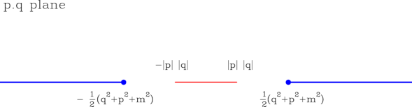
Figure 1: The complex $p\cdot q$ plane, for $p^{2},q^{2}$ both positive (space-like). The Euclidean integral (2.7) for the Nachtmann moment $\mu_{n}$ runs between $p\cdot q=-|p|\,|q|$ and $p\cdot q=+|p|\,|q|$, the Minkowski integral (2.9) runs along the cut from the threshold at $p\cdot q=\frac{1}{2}(q^{2}+p^{2}+m^{2})$ to $\infty$.

Following [4] we can relate the integral to Minkowski physics by allowing $p\cdot q$ to become complex, while keeping both $p^{2}$ and $q^{2}$ real and positive, see Fig.1. Ignoring the possible complications due to confinement, we expect the amplitude $T$ to have branch-points at the thresholds for producing on-shell quarks, at $p\cdot q=\pm\frac{1}{2}(q^{2}+p^{2}+m^{2})$, with cuts reaching out to infinity. We define the discontinuity across these cuts by

$$2\pi iD(p\cdot q,q^{2},p^{2},m)\equiv T_{\mu\mu}(p\cdot q+i\varepsilon,q^{2},p^{2})-T_{\mu\mu}(p\cdot q-i\varepsilon,q^{2},p^{2})\;.$$ (8)

For colour singlet hadrons this discontinuity is a physically measurable total cross-section, but of course the cross-section for deep inelastic scattering on an off-shell quark target is something we can only measure as a Gedankenexperiment. Assuming that $T$ is an analytic function of the complex variable $p\cdot q$ we can write down dispersion relations which give the result of the Euclidean integral (7) as an integral involving the discontinuity (valid for even $n$, $n\geq 2$).

$$\!\!\mu_{n}(q^{2},p^{2})=2\int_{\Theta}^{\infty}\!d(p\!\cdot\!q)\,\frac{D(p\cdot q,q^{2},p^{2})\;(q^{2})^{n}}{\left(p\cdot q+\sqrt{(p\cdot q)^{2}-p^{2}q^{2}}\right)^{n+1}}$$ (9)

where $\Theta$ is the threshold for the production of on-shell particles,

$$\Theta\equiv{\textstyle\frac{1}{2}}(q^{2}+p^{2}+m^{2})\;.$$ (10)

In general the Minkowski integral (9) is complicated, but in the Bjorken limit, when $(p\cdot q)^{2}\gg p^{2}q^{2}$, we can simplify (9) by changing to the integration variable

$$x\equiv\frac{q^{2}}{2p\cdot q}\;.$$ (11)

Eq. (9) becomes

$$\mu_{n}(q^{2},p^{2})=\int_{0}^{\frac{q^{2}}{2\Theta}}dx\;\frac{x^{n-1}D(p\cdot q,q^{2},p^{2})}{\left[\frac{1}{2}+\frac{1}{2}\sqrt{1-4\frac{p^{2}}{q^{2}}x^{2}}\;\;\right]^{n+1}}\ \to\int_{0}^{1}dx\;x^{n-1}D(p\cdot q,q^{2},p^{2})$$ (12)

and we see that the Nachtmann moment tends to a simple $x$ moment.

In the rest of this report we concentrate on the smallest interesting spin, $n=2$. From (12) we see that at large $q^{2}$, $\mu_{2}$ corresponds to $\langle x\rangle$.

In our discussion of Nachtmann moments we have assumed full rotation symmetry. However, lattice operators are classified under the hypercubic group, and will normally be mixtures of representations of the full Euclidean rotation group. The 22 operators present in the expansion of $W_{\mu\mu}$ fall into three hypercubic classes

spin 0,		spin 4,  + higher	8 operators
	spin 2,	spin 4,  + higher	13 operators
		spin 4,  + higher	1 operator

For our first look at spin 2, we simply keep all the operators in the middle group, and discard the others. The leading spin 2 operator (for $q\propto(1,1,1,1)$ ) has the form

$$\sum_{\mu\neq\nu}\overline{\psi}(\gamma_{\mu}D_{\nu}+\gamma_{\nu}D_{\mu})\psi$$ (13)

i.e. it is a symmetric, off-diagonal tensor.

We now reconstruct a projected spin 2 amplitude, $[T_{\mu\mu}]_{spin\ 2}$, by taking the product of the matrix elements of the 13 spin 2 operators with their Wilson coefficients, as determined in [1].

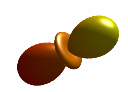
Figure 2: The 4-dimensional spherical harmonic $p^{2}q^{2}U_{2}(\cos\theta)=4(p\cdot q)^{2}-p^{2}q^{2}$. The main lobes point along the directions $\pm q$. There are nodes when $p$ is $60^{\rm o}$ and $120^{\rm o}$ from $q$; the equatorial ‘donut’ has the opposite sign to the main lobes.

Because we have averaged over quark spin and photon polarisations, the only direction left in our problem is $q\propto(1,1,1,1)$ and the only spin-2 4-d spherical harmonic that contributes is

$$p^{2}q^{2}U_{2}(\cos\theta)=4(p\cdot q)^{2}-p^{2}q^{2}\;,$$ (14)

which is illustrated in Fig.2. When we put in the fact that $q\propto(1,1,1,1)$

$$4(p\cdot q)^{2}-p^{2}q^{2}\to 2\left(p_{1}p_{2}+p_{1}p_{3}+\cdots+p_{3}p_{4}\right)q^{2}\;.$$ (15)

Spin 2 operators, such as (13), should have an expectation value proportional to (15).

We can find the $\mu_{2}$ for the quark from (7),

$$q^{2}\left[T_{\mu\mu}\right]_{spin2}=2\;\left(\sum_{\mu<\nu}p_{\mu}p_{\nu}\right)\;\mu_{2}\;,$$ (16)

so if we plot $q^{2}\left[T_{\mu\mu}\right]_{spin2}$ against $2\;\left(\sum_{\mu<\nu}p_{\mu}p_{\nu}\right)$ we should see a straight line passing through the origin, with a slope equal to $\mu_{2}$.

We have data for three different $q$ values, and from 15 to 32 $p$ values (depending on $q$), chosen to give a good coverage of directions, so we can see whether the projected amplitude really follows the spherical harmonic, and find $\mu_{2}$ for a quark.

3 Results

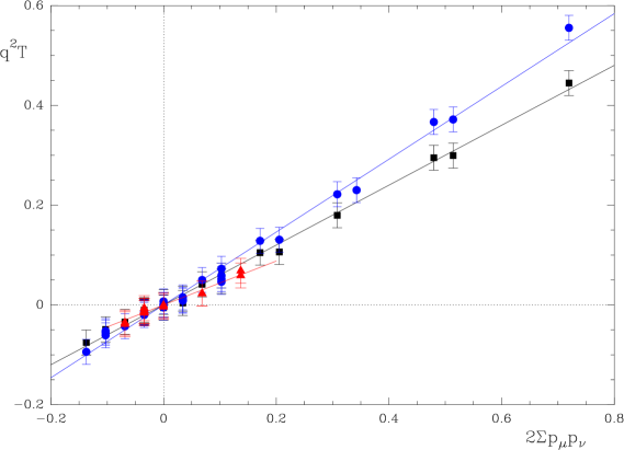
Figure 3: The trace $q^{2}\left[T_{\mu\mu}\right]_{spin2}$ plotted against $2\;\left(\sum_{\mu<\nu}p_{\mu}p_{\nu}\right)$, in lattice units. These points should fall on a straight line through the origin, with a slope proportional to $\mu_{2}$, the Nachtmann moment corresponding to $\langle x\rangle$, see eq.(2.16). The black squares are data from $q^{2}=\pi^{2}/(2.25a^{2})\approx 19$ GeV$\,{}^{2}$, blue circles, $q^{2}=\pi^{2}/(4a^{2})\approx 10.6$ GeV$\,{}^{2}$, red triangles $q^{2}=\pi^{2}/(9a^{2})\approx 4.7$ GeV$\,{}^{2}$.

In Fig.3 we show the spin-projected Compton amplitude plotted against $2\;\left(\sum_{\mu<\nu}p_{\mu}p_{\nu}\right)$. The quantity $2\;\left(\sum_{\mu<\nu}p_{\mu}p_{\nu}\right)$ is positive for momenta in the main lobe of the harmonic in Fig.2, zero for momenta in the node, and negative for momenta in the equatorial ring.

At each $q^{2}$ value the amplitudes follow a straight line rather closely. Several quarks have momenta at exactly $60^{\rm o}$ angle to $q$, these fall on the node of the spherical harmonic, (zero on the horizontal axis), and they have amplitudes very close to 0, as predicted. Data from all three $q$ values are plotted, we see that they scale fairly well. $q^{2}$ changes by a factor of 4, from 4.7 GeV² to 19 GeV².

Rough values for the Nachtmann moment $\mu_{2}$ (which is a measure of $\langle x\rangle$ at a scale $\sim q^{2}$) are

$q^{2}=4.7$ GeV2	$\mu_{2}=0.44(9)$
$q^{2}=10.6$ GeV2	$\mu_{2}=0.73(5)$
$q^{2}=19$ GeV2	$\mu_{2}=0.60(5)$

These values probably include fairly large lattice artefacts $\propto a^{2}q^{2}$. We will try to correct for these by looking at tree-level lattice artefacts, which might lead to significant numerical changes.

4 Conclusions and Prospects

We have seen how we can project out spin components for Nachtmann moment operator expansions. In the channel we looked at (spin 2), simply filtering on the lattice symmetry seems to work fairly well, we don’t see any sign of spin 4 contamination distorting the straight-line behaviour of Fig.3.

We don’t see any strong dependence of $\mu_{2}$ on the quark virtuality $p^{2}$, this may be a little unexpected.

There are several more things we could do. Here we have concentrated on the Nachtmann moment coming from the polarisation trace $W_{\mu\mu}$, we should also look at the moments for the other components of $W_{\mu\nu}$. Particularly interesting in the context of off-shell quarks would be to look at the OPE for $q_{\mu}W_{\mu\nu}q_{\nu}$. This should give a combination of operators which can be non-zero for off-shell quarks, but which should vanish on-shell. The three-point functions for this combination of operators should show contact terms, but no plateau or exponentially decaying terms.

The antisymmetric parts of the scattering tensor, $W_{\mu\nu}-W_{\nu\mu}$ contain the information needed to investigate spin-dependent structure functions. We have collected the data needed for this calculation.

From looking at our problem in tree level we see that $O(a^{2}q^{2})$ artifacts may be important in some channels. We want to investigate these artifacts further, and see whether we can use tree-level results to reduce their severity.

References

- [1] W. Bietenholz, proceedings of this conference. [arXiv:0910.2437 [hep-lat]]
- [2] S. Capitani, M. Göckeler, R. Horsley, P. E. L. Rakow and G. Schierholz, Phys. Lett. B 468 (1999) 150 [arXiv:hep-lat/9908029].
- [3] W. Bietenholz et al., PoS LAT2007 (2007) 159 [arXiv:0712.3772 [hep-lat]].
- [4] O. Nachtmann, Nucl. Phys. B 63 (1973) 237.
- [5] Abramowitz and Stegun, “Handbook of Mathematical Functions”, (Dover) 1972. Chapter 22.