Pure gauge glueballs at finite temperature

Abstract:

Pure gauge glueballs at finite temperature are investigated in a large temperature range from $0.3T_{c}$ to $1.9T_{c}$ on anisotropic lattices. Optimized glueball operators are used to obtain better signals. It is found in all 20 symmetry channels that the pole masses $M_{G}$ of glueballs remain almost constants when the temperature approaches the critical temperature $T_{c}$ from below, and start to reduce gradually with the temperature going above $T_{c}$. The glueball correlators in $0^{++}$, $0^{-+}$, and $2^{++}$ channels, are also analyzed based on the Breit-Wigner ansatz by assuming a thermal width $\Gamma$ to the pole mass $\omega_{0}$. While $\omega_{0}$’s are insensitive to $T$ in the whole temperature range, $\Gamma$’s exhibit distinct behavior below and above $T_{c}$: They are only few percents of $\omega_{0}$ when $T<T_{c}$, but grow abruptly when $T>T_{c}$ and reach values of roughly $\Gamma\sim\omega_{0}/2$ at $T\approx 1.9T_{c}$.

1 Introduction

Quantum Chromodynamics(QCD) is believed to be the fundamental theory of strong interaction. At finite temperature, QCD is usually described by two extreme pictures. One is with the weakly interacting meson gas in the low temperature regime and another is with perturbative Quark Gluon Plasma (QGP) in the high temperature regime. Lattice studies of QCD Equation of State (EOS) studies [1] indicate that the Steven-Boltzman ideal gas limit can be reached only at high $T$, and deconfined partons might be strongly interacting in the intermediate temperature range above $T_{c}$. This point is supported both by RHIC experiments and theoretically studies. On the one hand, the QGP observed by RHIC can be well described by the hydrodynamical model[2]. On the other hand, the lattice studies of meson correlators show that charmonia and light hadrons can survive in a temperature range beyond $T_{c}$ [3, 4, 5].

Since glueballs are predicted by QCD and well defined in pure Yang-Mills theory, their $T$-evolution is also a good probe to investigate the property of QCD matter in the deconfinement phase. In this work, we carry out a numerical lattice study on anisotropic lattices with much finer lattice in the temporal direction than in spatial ones. By varying the temporal extension of the lattice, we obtain a wide temperature range from $0.3T_{c}$ to $1.9T_{c}$. At each temperature, we take into account all the twenty $R^{PC}$ channels, with $PC=++,+-,-+,--$ the various parity-charge conjugate and $R=A_{1},A_{2},E,T_{1},T_{2}$ the irreducible representations of lattice symmetry group. For each $R^{PC}$, as in the zero temperature case [6, 7, 8], we implement smearing schemes and the variational method to acquire an optimal glueball operator which couples most to the ground state. In the data analysis stage, the correlators of these optimized operators are analyzed through two approaches. First, the thermal masses $M_{G}$ of glueballs are extracted in all the channels and all over the temperature range by fitting the correlators with a single-cosh function form, as is done in the standard hadron mass measurements. Thus the $T$-evolution of the thermal glueball spectrums are obtained. Secondly, with the respect that the finite temperature effects may result in mass shifts and thermal widths of glueballs, we also analyze the correlators in $A_{1}^{++}$, $A_{1}^{-+}$, $E^{++}$, and $T_{2}^{++}$ channels with the Breit-Wigner ansatz which assumes these glueballs thermal widths, say, changes $M_{G}$ into $\omega_{0}-i\Gamma$ in the spectral function (see below). It is expected that the temperature dependence of $\omega_{0}$ and $\Gamma$ can shed some light on the scenario of the QCD transition.

2 Numerical details

We adopt the tadpole improved Symanzik s action, which has been extensively used in the study of glueballs,

$$S_{IA}={\beta}{\{\frac{5}{3}\frac{\Omega_{sp}}{{\xi}u_{s}^{4}}+\frac{4}{3}\frac{\xi\Omega_{tp}}{u_{t}^{2}u_{s}^{2}}-\frac{1}{12}\frac{\Omega_{sr}}{{\xi}u_{s}^{6}}-\frac{1}{12}\frac{{\xi}\Omega_{str}}{u_{s}^{4}u_{t}^{2}}\}},$$ (1)

where $\beta$ is related to the bare QCD coupling constant, $\xi=a_{s}/a_{t}$ is the aspect ratio for anisotropy (we take $\xi=5$ in this work), $u_{s}$ and $u_{t}$ are the tadpole improvement parameters of spatial and temporal gauge links, respectively. Lattices are $24^{3}\times N_{t}$ with $\beta=3.2$, and $a_{s}=0.0878$fm, and the spatial volume $V\sim(2.1{\rm fm})^{3}$.

The deconfinement critical point is roughly determined by the susceptibility $\chi_{P}$ of Polyakov loops,

$$\chi_{P}=\langle\Theta^{2}\rangle-\langle\Theta\rangle^{2}$$ (2)

where $\Theta$ denotes the $Z(3)$ rotated Polyakov line,

$$\Theta = \left\{\ \begin{array}[]{ll}{\rm Re}P\exp[-2\pi i/3];&\arg P\in[\pi/3,\pi)\\ {\rm Re}P;&\arg P\in[-\pi/3,\pi/3)\\ {\rm Re}P\exp[2\pi i/3];&\arg P\in[-\pi,-\pi/3)\end{array}\right..$$ (6)

As illustrated in Fig. 1, the peak position is roughly at $N_{t}=38$, which corresponds to the critical temperature $T_{c}$. With the lattice spacing $a_{s}=0.0878$fm, $T_{c}$ is estimated to be $T_{c}=296$MeV. Based on this, we vary $N_{t}$ to obtain a temperature range from $T\sim 0.3T_{c}$ to $1.9T_{c}$, as listed in Table 1.

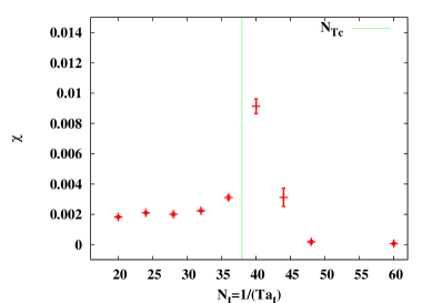
Figure 1: $\chi_{P}$ is plotted versus $N_{t}$ at $\beta=3.2$. There is a peak of $\chi_{P}$ near $N_{t}=40$.

For all the 20 $J^{PC}$ channels of glueballs, we take the following two steps to construct the optimal glueball operators which couple most to the ground states (More details can be found in Ref. [9] and Ref. [7, 8]). First, for a given gauge configuration, we generate six differently smeared copies, on each of which, four realizations of each $J^{PC}$ are established based on all the different spatially oriented Wilson loops of a set of loop prototypes [7]. As a result, we obtain a set of 24 different glueball operators, $\phi=\{\phi_{\alpha},\alpha=1,2,\ldots,24\}$, for each $J^{PC}$. At the second step, we carry out the variational method on each operator set $\phi$ to determine the specific combinational coefficients $\{v_{\alpha},\alpha=1,2,\ldots,24\}$ relevant to the ground state, such that the desired optimal operator is obtained as $\Phi=\sum\limits v_{\alpha}\phi_{\alpha}$. Practically at each temperature, after a thermalization of 10000 heatbath sweeps, the glueball operators are measured every three compound sweeps, each of which is composed of one heatbath and five micro-canonical over-relaxation(OR) sweeps. In the data analysis, the measurements are divided into $N_{\rm bin}$ bins of the size $n_{\rm mb}=400$ . Parameters $N_{\rm bin}$ and $n_{mb}$ at various temperature are also listed in Table 1.

$N_{t}$	$T/T_{c}$	$n_{\rm mb}$	$N_{\rm bin}$	$N_{t}$	$T/T_{c}$	$n_{\rm mb}$	$N_{\rm bin}$
128	0.30	400	24	36	1.05	400	40
80	0.47	400	30	32	1.19	400	56
60	0.63	400	44	28	1.36	400	40
48	0.79	400	40	24	1.58	400	40
44	0.86	400	44	20	1.90	400	40
40	0.95	400	40	–	–	–	–

Table 1: Temperature range and simulation parameters in this work.

3 Glueballs at finite temperature

Theoretically, under the periodic boundary condition in the temporal direction, the temporal correlators $C(t,T)$ at the temperature $T$ can be written in the spectral representation as

$$C(t,T) \equiv \frac{1}{Z(T)}{\rm Tr}\left(e^{-H/T}\Phi(t)\Phi(0)\right)$$ (7)

$$= \sum\limits_{m,n}\frac{|\langle n|\Phi|m\rangle|^{2}}{2Z(T)}\exp\left(-\frac{E_{m}+E_{n}}{2T}\right)\times\cosh\left[\left(t-\frac{1}{2T}\right)(E_{n}-E_{m})\right]$$

$$= \int\limits_{-\infty}^{\infty}d\omega\rho(\omega)K(\omega,T),$$

with a $T$-dependent kernel $K(\omega,T)=\frac{\cosh(\omega/(2T)-\omega t)}{\sinh(\omega/(2T))}$ and the spectral function,

$$\rho(\omega)=\sum\limits_{m,n}\frac{|\langle n|\Phi|m\rangle|^{2}}{2Z(T)}e^{-E_{m}/T}(\delta(\omega-(E_{n}-E_{m})-\delta(\omega-(E_{m}-E_{n})),$$ (8)

where $Z(T)$ is the partition function at $T$, and $E_{n}$ the energy of the thermal state $|n\rangle$ ($|0\rangle$ represents the vacuum state). In the zero-temperature limit($T\rightarrow 0$), due to the factor $\exp(-E_{m}/T)$, the spectral function $\rho(\omega)$ degenerates to

$$\rho(\omega)=\sum\limits_{n}\frac{|\langle 0|\Phi|n\rangle|^{2}}{2Z(0)}\left(\delta(\omega-E_{n})-\delta(\omega+E_{n})\right),$$ (9)

thus we have the function form of the correlation function, $C(t,T=0)=\sum\limits_{n}W_{n}e^{-E_{n}t}$ with $W_{n}=|\langle 0|\Phi|n\rangle|^{2}/Z(0)$. However, for any finite temperature (this is always the case for finite lattices), all the thermal states with the non-zero matrix elements $\langle m|\Phi|n\rangle$ may contribute to the spectral function $\rho(\omega)$. Intuitively in the confinement phase, the fundamental degrees of freedom are hadron-like modes, thus the thermal states should be multi-hadron states. If they interact weakly with each other, we can treat them as free particles at the lowest order approximation and consider $E_{m}$ as the sum of the energies of hadrons including in the thermal state $|m\rangle$. Since the contribution of a thermal state $|m\rangle$ to the spectral function is weighted by the factor $\exp(-E_{m}/T)$, apart from the vacuum state, the maximal value of this factor is $\exp(-M_{\rm min}/T)$ with $M_{\rm min}$ the mass of the lightest hadron mode in the system. As far as the quenched glueball system is concerned, the lightest glueball is the scalar, whose mass at the low temperature is roughly $M_{0^{++}}\sim 1.6$ GeV, which gives a very tiny weight factor $\exp(-M_{0^{++}}/T_{c})\sim 0.003$ at $T_{c}$ in comparison with unity factor of the vacuum state. That is to say, for the quenched glueballs, up to the critical temperature $T_{c}$, the contribution of higher spectral components beyond the vacuum to the spectral function are much smaller than the statistical errors (the relative statistical errors of the thermal glueball correlators are always a few percents) and can be neglected. As a result, the function form of $\rho(\omega)$ in Eq. 9 can be a good approximation for the spectral function of glueballs at least up to $T_{c}$. Accordingly, considering the finite extension of the lattice in the temporal direction, the function form of the thermal correlators can be approximated as

$$C(t,T)=\sum\limits_{n}W_{n}\frac{\cosh(M_{n}(1/(2T)-t))}{\sinh(M_{n}/(2T))},$$ (10)

which is surely the commonly used function form for the study of hadron masses at low temperatures on the lattice. As is always done, the glueball masses $M_{n}$ derived by this function are called the pole masses in this work.

3.1 The single-cosh fit

After the thermal correlators $C(t,T)$ are obtained, the pole masses of the ground state (or the lowest spectral component) can be extracted straightforwardly. For each $R^{PC}$ channel and at each temperature $T$, we first calculate the effective mass $M_{\rm eff}(t)$ as a function of $t$ by solving the equation

$$\frac{C(t+1,T)}{C(t,T)}=\frac{\cosh((t+1-N_{t}/2)a_{t}M_{\rm eff}(t))}{\cosh((t-N_{t}/2)a_{t}M_{\rm eff}(t))},,$$ (11)

and determine the time window $[t_{1},t_{2}]$ where $M_{\rm eff}$(t) has a plateau. In this time window, $C(t,T)$ is fitted through a single-cosh function form. Fig. 2 illustrates this procedure in $E^{++}$ channel.

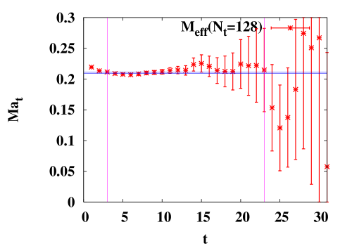
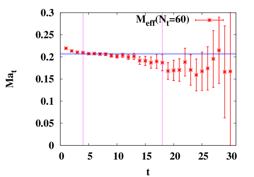
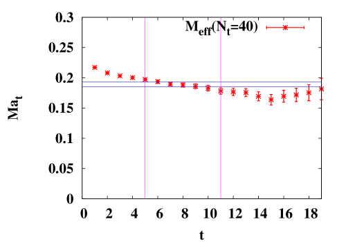
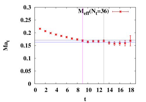
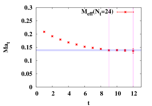
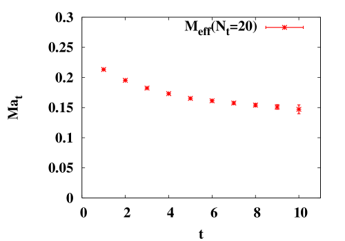
Figure 2: Effective masses at different temperatures in $E^{++}$ channel. Data points are the effective masses with jackknife error bars. The vertical lines indicate the time window $[t_{1},t_{2}]$ over which the single-cosh fittings are carried out, while the horizonal lines illustrate the best fit result of pole masses (in each panel the double horizonal lines represent the error band estimated by jackknife analysis)

In this work, the pole masses in all the 20 $R^{PC}$ channels are extracted at all the temperatures. The common feature of temperature dependence of pole masses is that, below $T_{c}$, the pole masses keep stable when varying the temperature, while above $T_{c}$, the pole masses decrease gradually and cannot be extracted beyond the temperature $T=1.6T_{c}$. Fig. 3 illustrates these hebaviors in $A_{1}^{++}$, $A_{1}^{-+}$, $E^{++}$, and $T_{2}^{++}$ channels. These results are different from the observation of a previous lattice study on glueballs where the observed pole-mass reduction start even at $T\simeq 0.8T_{c}$ [10].

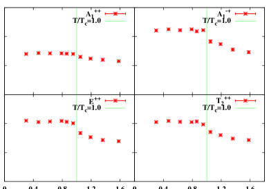
Figure 3: The $T$-dependence of pole masses $A_{1}^{++}$, $A_{1}^{-+}$ $E^{++}$, and $T_{2}^{++}$ glueballs.

3.2 Breit-Wigner analysis (BW)

Theoretically in the deconfined phase, gluons can be liberated from hadrons. However, the study of the equation of state shows that the state of the matter right above $T_{c}$ is far from a perturbative gluon gas. In other words, the gluons in the intermediate temperature above $T_{c}$ may interact strongly with each other and glueball-like resonances can be possibly formed. Thus different from bound states at low temperature, thermal glueballs can acquire thermal width due to the thermal scattering between strongly interacting gluons and the magnitudes of the thermal widths can signal the strength of these type of interaction at different temperature.

By assuming glueballs thermal widths, we also adopt the Breit-Wigner ansatz [10] to analyze the thermal correlators once more. First, we treat thermal glueballs as resonance objects which correspond to the poles (denoted by $\omega=\omega_{0}-i\Gamma$) of the retarded and advanced Green functions in the complex $\omega-$plane. $\omega_{0}$ is called the mass of the resonance glueball and $\Gamma$ its thermal width in this work. Secondly, we assume that the spectral function $\rho(\omega)$ is dominated by these resonance glueballs. With these respects, the thermal correlators can be parameterized as [9, 10]

$$g_{\Gamma}(t) = A\left[{\rm Re}\left(\frac{\cosh((\omega_{0}+i\Gamma)(\frac{1}{2T}-t))}{\sinh(\frac{(\omega_{0}+i\Gamma)}{2T})}\right)\right.$$ (12)

$$+ \left.2\omega_{0}T\sum\limits_{n=1}^{\infty}\cos\left(2\pi nTt\right)\left\{\frac{1}{(2\pi nT+\Gamma)^{2}+\omega_{0}^{2}}-(n\rightarrow-n)\right\}\right].$$

In the data analysis, the effective mass $\omega_{0}^{\rm{eff}}(t)$ and effective width $\Gamma^{\rm{eff}}(t)$ are obtained first by solving the equation array,

$${g_{\Gamma}(t)}/{g_{\Gamma}(t+1)} = {C(t,T)}/{C(t+1,T)}$$

$${g_{\Gamma}(t+1)}/{g_{\Gamma}(t+2)} = {C(t+1,T)}/{C(t+2,T)},$$ (13)

where $C(t,T)$ is the measured correlator, then the simultaneous plateau region of $\omega_{0}(t)$ and $\Gamma(t)$ gives the fit window $[t_{1},t_{2}]$ where the fit is carried out. This procedure in $T_{2}^{++}$ channel is shown in Fig. 4 for instance.

(a) $N_{t}=128$($T/T_{c}=0.32$)	(b) $N_{t}=36$($T/T_{c}=1.09$)	(c) $N_{t}=20$($T/T_{c}=1.97$)

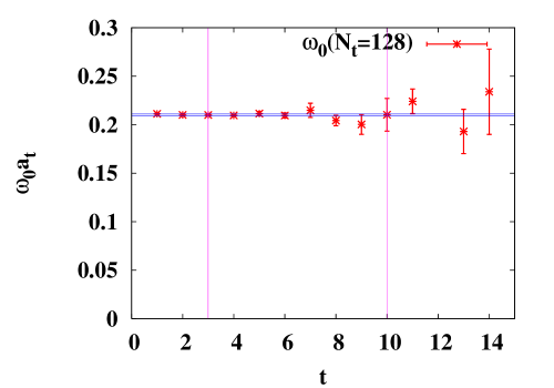
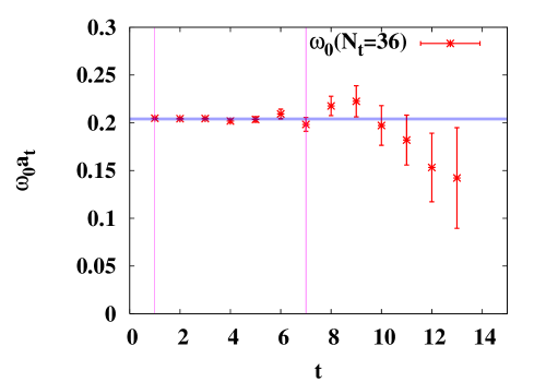
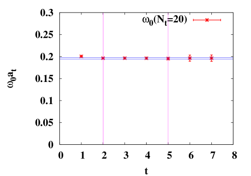
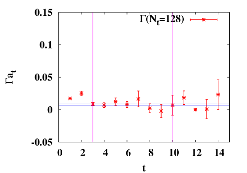
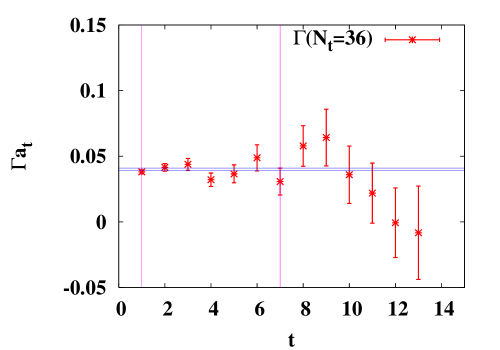
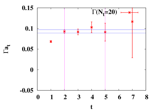
Figure 4: Determinations of the fit range $[t_{1},t_{2}]$ in $T_{2}^{++}$ channel at $N_{t}=$ 128, 36, and 20. In each row, $\omega_{0}^{\rm(eff)}(t)$ and $\Gamma^{\rm(eff)}(t)$ are plotted by data points with jackknife error bars. $[t_{1},t_{2}]$ are chosen to include the time slices between the two vertical lines, where $\omega_{0}^{\rm(eff)}(t)$ and $\Gamma^{\rm(eff)}(t)$ show up plateaus simultaneously. The best fit results of $\omega_{0}$ and $\Gamma$ through the function $g_{\Gamma}(t)$ are illustrated by the horizonal lines.

The main feature of the best fit $\omega_{0}$ and $\Gamma$ in $A_{1}^{++},A_{1}^{-+},E^{++}$, and $T_{2}^{++}$ channels is illustrated in Figure 5: First, $\omega_{0}$’s are insensitive to $T$, or more specifically, the reduction of $\omega_{0}$ at the highest temperature $T=1.90T_{c}$ are less than $5\%$. Secondly, $\Gamma$’s are small and do not vary much below $T_{c}$, but increase abruptly when the temperature passes $T_{c}$ and reach to values $\sim\omega_{0}/2$ at $T=1.90T_{c}$. These features can be easily seen in Fig. 5, where the behaviors of $\omega_{0}$ and $\Gamma$ with respect to the temperature $T$ are plotted for all the four channels.

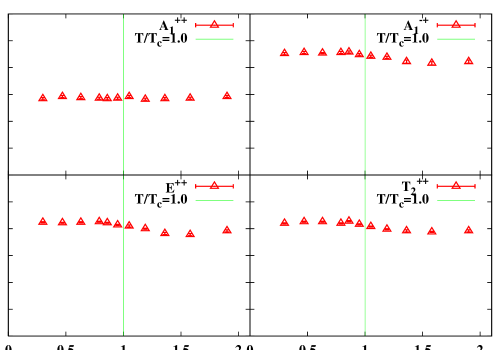
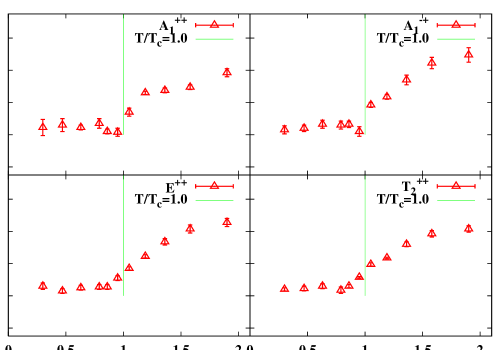
Figure 5: $\omega_{0}$’s and $\Gamma$’s are plotted versus $T/T_{c}$ for $A_{1}^{++}$, $A_{1}^{-+}$ $E^{++}$, and $T_{2}^{++}$ channels. The vertical lines indicate the critical temperature.

4 Summary and conclusion

In the pure SU(3) gauge theory, the thermal correlators in all the 20 symmetry channels are calculated on anisotropic lattices in the temperature range from 0.3 $T_{c}$ to 1.9$T_{c}$. Both the single-cosh fit and BW analysis show that glueballs can survive up to 1.9$T_{c}$. Our results are consistent with that of the studies of EOS and charmonia  [3, 4, 12, 13]. In BW analysis, glueball masses keep stable when the temperature increasing, and the thermal widths of glueballs becomes larger and larger above $T_{c}$. It seems that in the intermediate T range, the state of matter are dominated by strongly interacting gluons. Gluons interact with each other strongly enough to form glueball-like resonances, in the mean time, glueballs can also decay into gluons. At a given temperature, these two procedure reach the thermal equilibrium. The thermal widths signal the interaction strength.

This work is supported in part by NSFC (Grant No. 10575107, 10675005, 10675101, 10721063, and 10835002) and CAS (Grant No. KJCX3-SYW-N2 and KJCX2-YW-N29). The numerical calculations were performed on DeepComp 6800 supercomputer of the Supercomputing Center of Chinese Academy of Sciences, Dawning 4000A supercomputer of Shanghai Supercomputing Center, and NKstar2 Supercomputer of Nankai University.

References

- [1] P. Petreczky, hep-lat/0409139; F. Karsch, Lect. Notes Phys. 583, 209 (2002), arXiv:hep-lat/0106019; D.E. Miller, Acta Physica Polonica B 28, 2937 (1997), arXiv:hep-ph/9807304.
- [2] STAR Collaboration: K.H. Ackermann, et al., Phys. Rev. Lett. 86, 402 (2001), arXiv:nucl-ex/0009011 .
- [3] M. Asakawa and T. Hatsuda, Phys. Rev. Lett. 92, 012001 (2004), arXiv:hep-lat/0308034.
- [4] S. Datta, F. Karsch, P. Petreczky, and I. Wetzorke, Phys. Rev. D 69, 094507 (2004), arXiv:hep-lat/0312037; S. Datta, F. Karsch, P. Petreczky, and I. Wetzorke, J.Phys. G 30, S1347 (2004).
- [5] M. Asakawa et al., Nucl. Phys. A 715 863 (2003).
- [6] C.J. Morningstar and M. Peardon, Phys. Rev. D 56, 4043 (1997).
- [7] C.J. Morningstar and M. Peardon, Phys. Rev. D 60, 034509 (1999).
- [8] Y. Chen et al., Phys. Rev. D 73, 014516 (2006).
- [9] X.-F. Meng et al. [CLQCD Collaboration], arXiv:0903.1991 [hep-lat]
- [10] N. Ishii, H. Suganuma, and H. Matsufuru, Phys. Rev. D 66, 094506 (2002), arXiv:hep-lat/0206020 ; N. Ishii, H. Suganuma, and H. Matsufuru, Phys. Rev. D 66, 014507 (2002), arXiv:hep-lat/0309102.
- [11] W. Liu et al., Mod. Phys. Lett. A 21, 2313 (2006).
- [12] S. Gottlieb et al., Phys. Rev. Lett. 59, 2247 (1987); S. Gottlieb et al., Phys. Rev. D 38, 2888 (1988); S. Gottlieb et al., Phys. Rev. D 55, 6852 (1997).
- [13] C. DeTar, Phys. Rev. D 32, 276 (1985); Phys. Rev. D 37, 2328 (1988); G. Boyd, S. Gupta, F. Karsch, and E. Laermann, Z. Phys. C 64, 331 (1994); H. Iida, T. Doi, N. Ishii, H. Suganuma, and K. Tsumura, Phys. Rev. D 74, 074502 (2006), arXiv:hep-lat/0602008 ; A. Jakovac, P. Petreczky, K. Petrov, and A. Velytsky, PoS(JHW 2005), arXiv:hep-lat/0603005; B. Berg and A. Billoire, Nucl. Phys. A 783, 477 (2007); Ph. de Forcrand et al.[QCD-TARO Collaboration], Phys. Rev. D 63, 054501 (2001); T. Umeda, R. Katayama,O. Miyamura and H. Matsufuru, Int. J. Mod. Phys. A 16, 2215 (2001).