Electromagnetic Radiations
as a Fluid Flow

Abstract

We combine Maxwell’s equations with Eulers’s equation, related to a velocity field of an immaterial fluid, where the density of mass is replaced by a charge density. We come out with a differential system able to describe a relevant quantity of electromagnetic phenomena, ranging from classical dipole waves to solitary wave-packets with compact support. The clue is the construction of an energy tensor summing up both the electromagnetic stress and a suitable mass tensor. With this right-hand side, explicit solutions of the full Einstein’s equation are computed for a wide class of wave phenomena. Since our electromagnetic waves may behave and interact exactly as a material fluid, they can create vortex structures. We then explicitly analyze some vortex ring configurations and examine the possibility to build a model for the electron.

Keywords: Electromagnetism, Euler’s equation, Einstein’s equation, photons, vortex rings.

PACS: 03.50.De, 04.20.Jb, 12.10.-g, 47.32.cf

1 Introduction

Since the advent of the theory of electromagnetic fields, more than a century ago, waves have been described as a kind of energy flow, governed by suitable transport equations in vector form, namely Maxwell’s equations. The original publications (see [19] and [20]), in a way that nowadays may seems naif, actually refer to electric and magnetic phenomena using mechanical terms, such as tension, stress, pressure and vortices, in association with some ‘imaginary substance’.

It turns out that, in void, the electric and magnetic fields (${\bf E}$ and ${\bf B}$, respectively) are transversally oriented with respect to the direction of propagation, and their envelope produces a sequence of wave-fronts. This is in agreement with the fact that the energy develops according to the evolution of the vector product ${\bf E}\times{\bf B}$, otherwise known as Poynting vector.

On the other hand, the dynamical behavior of a compressible non viscous fluid is well described by Euler’s equation, where, in principle, the velocity vector field (denoted by ${\bf V}$) might not be necessarily related to a real material fluid. In particular, one could replace the mass density by a sort of charge density. Therefore, the temptation to describe electromagnetic and velocity fields, through a combination of the respective modelling equations, is well motivated.

We are going to present a system of equations in the three independent vector unknowns: $({\bf E},{\bf B},{\bf V})$. In pure void, the electric and magnetic fields follow the Faraday’s law together with the Ampère’s law, where a current, flowing at velocity ${\bf V}$, is supposed to be naturally associated with the wave. In order to close the system, the third relation is the Euler’s equation for ${\bf V}$, containing an added forcing term ${\bf E}+{\bf V}\times{\bf B}$, perfectly analogous to that characterizing the Lorentz’s law. In this way, the three entities $({\bf E},{\bf B},{\bf V})$ turn out to be strictly entangled.

Despite the appearance, the new model allows for a very large space of solutions. Moreover, it displays numerous conservation and invariance properties, all deducible from a standard analysis. An interesting invariant subspace of solutions is the one where the third equation is reduced to ${\bf E}+{\bf V}\times{\bf B}=0$, which means that no acceleration is acting on the wave, and the corresponding ‘flow’ is somehow laminar. For this circumstance, the solutions, called free-waves, perfectly follow the laws of geometrical optics, ruled by the eikonal equation. Together with other known solutions, free-waves also include solitary electromagnetic waves with compact support almost of any shape, intensity, frequency and polarization. Such a result is clearly important, since it reopens the path to a serious discussion, based on a deterministic analysis, on crucial issues as the structure of photons, the duality wave-particle and the quantum properties of matter.

Far more complicated solutions (not of the free-wave type) are however possible. Since our electromagnetic radiations actually behave as a fluid, they can be constrained to evolve in bounded regions of space, similar for instance to vortex rings. According to the model equations, rotating photons in a vortex structure may carry a charge and deform, via Einstein’s equation, the local geometry of the space-time in order to create a gravitational environment assimilable to the presence of mass. The same metric space is responsible for the stability of such a wave, obliged in this way to develop along self-created geodesics. This leaves us with the conjecture that some stable elementary particles (as for instance the electron) could be made by rotating photons, an idea that has been put forward by many authors in the past, although with not too much recognition, basically due to the lack of a sufficient theoretical description of electromagnetic phenomena, able to go beyond the classical linear Maxwellian approach. With the help of the new material collected here, we examine this aspect in the last section.

This paper is a review and a reorganization of the results presented in [11], and contains additional new material. The presentation follows an inverse path, and the equations are first derived in covariant form and successively deduced in the flat space. The general relativity framework is however the key point to understand the structure of the solutions, especially in the case of constrained waves. The entire theory comes out as a consequence of a wise choice of the right-hand side tensor in the formulation of Einstein’s equation. This combines in the proper manner the electromagnetic stress tensor and a mass type tensor, where the density is referred to the electric field. In the subspace of free-waves, by generalizing the results given in [11], we are able to write down explicit general solutions of the Einstein’s equation. As a final step, we will derive a notion of mass density, that is going to be zero in the average for free-waves (and photons) and positive for electrons.

2 The right-hand side tensor

Let us fix the notation by introducing the Einstein’s equation:

$$R_{\alpha\beta}~{}-~{}{\textstyle\frac{1}{2}}g_{\alpha\beta}R~{}=~{}-\chi T_{\alpha\beta}$$ (1)

where $R_{\alpha\beta}$ is the Ricci tensor, $R$ the scalar curvature (the trace of $R_{\alpha\beta}$) and $\chi$ a positive adimensional constant. The signature of the metric space $g_{\alpha\beta}$ will be $(+,-,-,-)$. The given constant $\chi$, that will be estimated at the end of section 6, has nothing in common with the gravitational constant $G$.

As anticipated in the introduction, the main ingredient of our theory, is the choice of the right-hand side tensor. We set:

$$T_{\alpha\beta}~{}=~{}\frac{\mu}{c^{4}}\Big{(}-\mu U_{\alpha\beta}+M_{\alpha\beta}\Big{)}$$ (2)

where $c$ is the speed of light and $\mu$ is a constant, dimensionally equivalent to a charge divided by a mass (see (62)). In (2) we find the usual electromagnetic stress tensor:

$$U_{\alpha\beta}~{}=~{}-g^{\gamma\delta}F_{\alpha\gamma}F_{\beta\delta}+{\textstyle{\frac{1}{4}}}g_{\alpha\beta}F_{\gamma\delta}F^{\gamma\delta}$$ (3)

with

$$F_{\alpha\beta}~{}=~{}\nabla_{\alpha}A_{\beta}-\nabla_{\beta}A_{\alpha}$$ (4)

where $A_{\alpha}$ is the electromagnetic 4-vector potential (energy/charge) and $\nabla_{\alpha}$ denotes the covariant derivative. Although it is not strictly requested, $A_{\alpha}$ satisfies the Lorenz gauge relation:

$$\nabla_{\alpha}A^{\alpha}~{}=~{}0$$ (5)

In (2) we also find a kind of mass tensor:

$$M_{\alpha\beta}~{}=~{}\rho V_{\alpha}V_{\beta}-g_{\alpha\beta}p$$ (6)

where $V_{\alpha}$ is velocity 4-vector, $\rho$ plays the role of a density and $p$ is similar to a pressure. Dimensionally, $\rho$ and $p$ are taken in order to conform with the setting in (2), therefore they will not correspond to the usual entities of classical fluid dynamics. Moreover, differently from what it is generally supposed (see for instance [10], p.91), no direct relations between $\rho$ and $p$ are a priori requested.

This way of building $T_{\alpha\beta}$ characterizes the whole theory. We remark (and this is an important key point) that $U_{\alpha\beta}$ in (2) appears with the opposite sign. The reason for this choice will be clear as we proceed in the exposition.

Concerning the vector field $V_{\alpha}$, we shall make the following assumption:

$$g^{\alpha\beta}V_{\alpha}V_{\beta}~{}=~{}0$$ (7)

that is equivalent to an eikonal equation for suitable propagating wave-fronts.

A first important relation is obtained by evaluating the trace of (1). This gives:

$$p~{}=~{}\frac{c^{4}}{4\chi\mu}R$$ (8)

In computing (8) we considered that both the traces of $U_{\alpha\beta}$ and $\rho V_{\alpha}V_{\beta}$ are zero. In the first case this is a known property of the electromagnetic stress tensor. In the second case it is a straightforward consequence of relation (7). Equation (8) relates curvature and pressure. Wave-fronts travelling unperturbed, without developing interstitial pressure, actually move in a space with zero scalar curvature, and vice versa (see section 4).

Let us then derive from (1) a set of covariant equations. In order to have compatibility with the left-hand side in (1), the most important relation to be satisfied is:

$$\nabla_{\beta}T^{\alpha\beta}~{}=~{}0$$ (9)

yielding the set of modelling equations. Due to the special expression of $T_{\alpha\beta}$, the energy conservation property (9) mixes up electromagnetic and mechanical terms in a very natural way. Thus, we start by observing that (see for instance [10] or [22]):

$$\nabla_{\beta}U^{\alpha\beta}~{}=~{}g^{\alpha\gamma}F_{\gamma\delta}(\nabla_{\beta}F^{\delta\beta})$$ (10)

$$\nabla_{\beta}M^{\alpha\beta}~{}=~{}\rho G^{\alpha}+\nabla_{\beta}(\rho V^{\beta})V^{\alpha}-g^{\alpha\beta}\nabla_{\beta}p~{}~{}~{}~{}{\rm with}~{}~{}G^{\alpha}=V^{\gamma}\nabla_{\gamma}V^{\alpha}$$ (11)

Thus, according to (9), by summing up the above expressions, one must have:

$$-~{}\mu g^{\alpha\gamma}F_{\gamma\delta}(\nabla_{\beta}F^{\delta\beta})~{}+~{}\rho G^{\alpha}~{}+~{}\nabla_{\beta}(\rho V^{\beta})V^{\alpha}~{}-~{}g^{\alpha\beta}\nabla_{\beta}p~{}=~{}0$$ (12)

By adding and subtracting the term $~{}(\mu\rho/c)g^{\alpha\gamma}F_{\gamma\delta}V^{\delta}=(\mu\rho/c)F^{\alpha\delta}V_{\delta}$, equation (12) becomes:

$$\mu g^{\alpha\gamma}F_{\gamma\delta}\Big{(}-\nabla_{\beta}F^{\delta\beta}-\frac{\rho}{c}V^{\delta}\Big{)}~{}+~{}\rho\Big{(}G^{\alpha}+\frac{\mu}{c}F^{\alpha\delta}V_{\delta}\Big{)}~{}~{}~{}~{}~{}~{}~{}~{}~{}~{}~{}~{}~{}~{}$$

$$~{}~{}~{}~{}~{}~{}~{}~{}~{}~{}~{}~{}~{}~{}~{}~{}+~{}\nabla_{\beta}(\rho V^{\beta})V^{\alpha}~{}-~{}g^{\alpha\beta}\nabla_{\beta}p~{}=~{}0$$ (13)

Hence, in order to obtain (13), a sufficient condition is to impose the following set of equations:

$$c~{}\nabla_{\beta}F^{\delta\beta}~{}=~{}-\rho V^{\delta}$$ (14)

$$\rho\Big{(}G^{\alpha}+\frac{\mu}{c}F^{\alpha\delta}V_{\delta}\Big{)}~{}=~{}\nabla^{\alpha}p$$ (15)

that, being written in covariant form, are, in principle, admissible in any geometric environment, but, hopefully, in the metric spaces compatible with relation (7). Equation (14) is the Ampère law and (15) is the Euler’s equation for a certain velocity field (not corresponding to a material fluid). In truth, in order to get (13), one should also impose the following continuity equation:

$$\nabla_{\beta}(\rho V^{\beta})~{}=~{}0$$ (16)

but this is a consequence of equation (14). In fact, by taking the 4-divergence of (14), one has: $c\nabla_{\delta}(\nabla_{\beta}F^{\delta\beta})=0=\nabla_{\delta}(\rho V^{\delta})$, resulting from the anti-symmetry of the tensor $F^{\delta\beta}$.

There is an interesting compatibility relation to be remarked. First, thanks to (7), one recovers that:

$$G^{\alpha}V_{\alpha}~{}=~{}{\textstyle{\frac{1}{2}}}(G^{\alpha}V_{\alpha}+G_{\alpha}V^{\alpha})~{}=~{}{\textstyle{\frac{1}{2}}}(V^{\gamma}\nabla_{\gamma})(V_{\alpha}V^{\alpha})~{}=~{}0$$ (17)

Then, due to the anti-symmetry of $F^{\delta\beta}$, (15) implies:

$$V_{\alpha}\nabla^{\alpha}p~{}=~{}0$$ (18)

which is a sort of conservation property for $p$ (a kind of Bernoulli’s principle, if one considers that $p=p+\frac{1}{2}\rho V_{\alpha}V^{\alpha}$).

The equations (14) and (15), together with the equation of state (8), are the foundations of our theory. In principle, one could obtain (9) without necessarily enforcing (14) and (15). However, we believe that all the most relevant phenomena can be described through the two differential equations written above.

3 The model equations in Minkowski space

To better understand what is happening we can specialize equations (14) and (15) in the case of a flat metric space $~{}g_{\alpha\beta}={\rm diag}\{1,-1,-1,-1\}$, in the Cartesian coordinate system $(ct,x_{1},x_{2},x_{3})$.

We start from the potential $(A_{0},A_{1},A_{2},A_{3})=(-\Phi,{\bf A})$ and through (4), considering that $\nabla_{\alpha}=(\frac{1}{c}\frac{\partial}{\partial t},\nabla)$, we obtain the electromagnetic tensor (see [10], section 24, or [3], section 5.2):

$$F_{\alpha\beta}~{}=~{}\left(\begin{array}[]{c @{\hspace{.5cm}} c @{\hspace{.5cm}} c @{\hspace{.5cm}} c}0\hfil\hskip 14.22636pt&-E_{1}\hfil\hskip 14.22636pt&-E_{2}\hfil\hskip 14.22636pt&-E_{3}\\ E_{1}\hfil\hskip 14.22636pt&0\hfil\hskip 14.22636pt&cB_{3}\hfil\hskip 14.22636pt&-cB_{2}\\ E_{2}\hfil\hskip 14.22636pt&-cB_{3}\hfil\hskip 14.22636pt&0\hfil\hskip 14.22636pt&cB_{1}\\ E_{3}\hfil\hskip 14.22636pt&cB_{2}\hfil\hskip 14.22636pt&-cB_{1}\hfil\hskip 14.22636pt&0\end{array}\right)$$ (19)

where ${\bf E}=(E_{1},E_{2},E_{3})$ is the standard electric field and ${\bf B}=(B_{1},B_{2},B_{3})$ is the magnetic field. The above construction is true by virtue of the setting (see (4)):

$${\bf B}~{}=~{}\frac{1}{c}~{}{\rm curl}{\bf A}~{}~{}~{}~{}~{}~{}~{}~{}~{}~{}~{}~{}~{}{\bf E}~{}=~{}-\frac{1}{c}\frac{\partial\bf A}{\partial t}~{}-~{}\nabla\Phi$$ (20)

In particular, we have:

$$\frac{\partial{\bf B}}{\partial t}~{}=~{}-{\rm curl}{\bf E}~{}~{}~{}~{}~{}~{}~{}~{}~{}~{}~{}~{}~{}~{}~{}~{}~{}~{}{\rm div}{\bf B}~{}=~{}0$$ (21)

as a direct consequence of (20). The contravariant tensor $F^{\alpha\beta}$ is obtained from $F_{\alpha\beta}$ by replacing ${\bf E}$ by $-{\bf E}$.

Without loss of generality, we can set $V^{0}=-c$, so that, from (14) with $\delta=0$, we deduce: $\rho=\nabla_{\beta}F^{0\beta}={\rm div}{\bf E}$. Denoting by ${\bf V}=(V_{1},V_{2},V_{3})$ the velocity field, by (7) one obtains $~{}V_{\alpha}=(-c,{\bf V})~{}$ and $~{}V^{\alpha}=(-c,-{\bf V})$. Finally we get:

$$\frac{\partial{\bf E}}{\partial t}~{}=~{}c^{2}{\rm curl}{\bf B}~{}-~{}\rho{\bf V}$$ (22)

$$\rho\left(\frac{D{\bf V}}{Dt}~{}+~{}\mu({\bf E}+{\bf V}\times{\bf B})\right)~{}=~{}-\nabla p$$ (23)

$$\frac{\partial p}{\partial t}~{}=~{}\mu\rho({\bf E}\cdot{\bf V})$$ (24)

where $~{}\frac{D}{Dt}{\bf V}=\frac{\partial}{\partial t}{\bf V}+({\bf V}\cdot\nabla){\bf V}~{}$ is the substantial derivative, so that (23) ends up to be the Euler’s equation. Here equation (22) comes from (14) for $\delta=1,2,3,$ equation (23) comes from (15) for $\alpha=1,2,3,$ and equation (24) comes from (15) for $\alpha=0$. In addition, one has the continuity equation:

$$\frac{\partial\rho}{\partial t}~{}=~{}-{\rm div}(\rho{\bf V})$$ (25)

that is easily derived either from (16) or by taking the divergence of (22).

The equations (8) and (7) are not valid in this context, since they are strongly related to the fact that $g_{\alpha\beta}$ is solution of (1), which is not true in the simplified case we are examining. The solutions to (22)-(24) are however important to set up the tensor $F_{\alpha\beta}$ in (4), which may be computed using partial derivatives in place of covariant derivatives. This enables us to build the tensor (2) for a generic $g_{\alpha\beta}$ to be used as a right-hand side in (1).

An even more simplified version is obtained by requiring $D{\bf V}/Dt=0$ and $p=0$ in (23):

$$\frac{\partial{\bf E}}{\partial t}~{}=~{}c^{2}{\rm curl}{\bf B}~{}-~{}\rho{\bf V}$$ (26)

$$\frac{\partial{\bf B}}{\partial t}~{}=~{}-{\rm curl}{\bf E}$$ (27)

$${\rm div}{\bf B}~{}=~{}0$$ (28)

$${\bf E}~{}+~{}{\bf V}\times{\bf B}~{}=~{}0$$ (29)

where $\rho={\rm div}{\bf E}$, and ${\bf V}$ is a velocity vector field satisfying $|{\bf V}|=c$. Note that (7) is now true. The field ${\bf V}$ is oriented as the vector field ${\bf E}\times{\bf B}$. Now (8) is also correct, since the property $R=0$ is compatible with the flatness of the space. Note that relation (29) is certainly satisfied for all electromagnetic waves where ${\bf E}$ is orthogonal to ${\bf B}$ and $|{\bf E}|=|c{\bf B}|$. Moreover, from (29) we get ${\bf E}\cdot{\bf V}=0$, that is in agreement with (24), since $p$ is identically zero. Take into account, however, that the flat metric does not satisfy (1), since in this case one has $R_{\alpha\beta}=0$, in contrast to the fact that $T_{\alpha\beta}\not=0$.

This set of equations produces a closed subset of solutions called free-waves, that contains all the electromagnetic phenomena in vacuum travelling undisturbed according to the rules of geometrical optics. Indeed, if ${\bf V}=\nabla\Psi$ is a gradient, then the relation $|{\bf V}|=|\nabla\Psi|=c$ is the eikonal equation. This subspace includes solitary waves with compact support, perfect spherical waves, and many other solution non obtainable with the classical Maxwell’s setting. In this case, equation (26) comes from finding the stationary points of the standard Lagrangian of the electromagnetism, under the condition $~{}A_{\alpha}V^{\alpha}=0~{}$ on the potentials (see [14]). Moreover, (26) is invariant under Lorentz transformations (see [11], section 2.6).

The subset of free-waves is characterized in covariant form by the following expression, deduced from (15) for $p=0$ and $G^{\alpha}=0$:

$$F^{\alpha\delta}V_{\delta}~{}=~{}0$$ (30)

that brings to (29) and ${\bf E}\cdot{\bf V}=0$. It can also be proven that both (25) and (30) are invariant under Lorentz transformations.

The triplet $({\bf E},{\bf B},{\bf V})$ turns out to be right-handed (in the right-handed reference frame $(x,y,z)$). There is however an alternative path, that brings to left-handed triplets. It is enough to replace (20) by:

$${\bf B}~{}=~{}-\frac{1}{c}~{}{\rm curl}{\bf A}~{}~{}~{}~{}~{}~{}~{}~{}~{}~{}~{}~{}~{}{\bf E}~{}=~{}-\frac{1}{c}\frac{\partial\bf A}{\partial t}~{}-~{}\nabla\Phi$$ (31)

and rewrite all the equations with $-{\bf B}$ in place of ${\bf B}$. We get in this way a completely new set of electromagnetic waves that have a specular image with respect to the classical one.

4 Explicit solutions

In the case of free-waves explicit expressions of the metric tensor $g_{\alpha\beta}$ are available. The results we are going to show generalize those given in [11].

Let us assume the following form for the potentials:

$$A_{\alpha}~{}=~{}\Big{(}-f(x,y)\tau(\xi),~{}0,~{}0,~{}f(x,y)\tau(\xi)\Big{)}$$ (32)

Here we are in Cartesian coordinates $(x_{0},x_{1},x_{2},x_{3})=(ct,x,y,z)$ and we set $\xi=z-ct$. The two functions $f$ and $\tau$ are arbitrary.

With this setting, we obtain the electromagnetic fields:

$${\bf E}=(-f_{x}\tau,~{}-f_{y}\tau,~{}0)~{}~{}~{}~{}~{}~{}~{}~{}~{}~{}~{}~{}{\bf~{}B}=c^{-1}(f_{y}\tau,~{}-f_{x}\tau,~{}0)$$ (33)

where $f_{x}=\partial f/\partial x$ and $f_{y}=\partial f/\partial y$. Thus, we are in presence of fronts parallel to the plane $(x,y)$ and evolving in the direction of the $z$ axis at speed $c$. Plane waves are obtained when $f$ is of the form $ax+by$, for some constants $a$ and $b$. The case when $f$ has compact support is quite interesting, since it give rise to self-contained solitary waves, travelling straightly at the speed of light (photons). These solutions do not belong to the Maxwellian theory (see also [13] and [14]). By defining $V_{\alpha}=(V_{0},{\bf V})=(-c,0,0,c)$, the entire set of equations (26)-(29) is satisfied in the flat space. Thus, we can also write $\xi=z-V_{3}t$. We observe that ${\rm div}{\bf B}$ is automatically zero, while we do not expect $~{}{\rm div}{\bf E}=-(f_{xx}+f_{yy})\tau~{}$ to be zero.

For any arbitrary (nonzero) function $s$ of the variable $x+y$, we look for a metric tensor having the following structure:

$$g_{00}=1~{}~{}~{}~{}~{}~{}~{}g_{11}=-f^{2}_{x}\sigma^{2}-s^{2}~{}~{}~{}~{}~{}~{}g_{12}=g_{21}=-f_{x}f_{y}\sigma^{2}-s^{2}$$

$$~{}g_{22}=-f^{2}_{y}\sigma^{2}-s^{2}~{}~{}~{}~{}~{}~{}~{}~{}g_{33}=-1$$ (34)

being the other entries equal to zero. Here $\sigma$ is a function of the variable $\xi$. Note that, in this situation and in accordance to (7), we have:

$$V^{\alpha}V_{\alpha}~{}=~{}0~{}~{}~{}~{}{\rm and}~{}~{}~{}~{}V^{\alpha}A_{\alpha}~{}=~{}0$$ (35)

with $V^{\alpha}=(-c,0,0,-c)$.

The determinant of the metric tensor is: $g=-[s(f_{x}-f_{y})\sigma]^{2}$. For this reason, it is necessary that $s\not=0$. We have:

$$F_{\alpha\beta}=\tau\left(\begin{array}[]{c @{\hspace{.2cm}} c @{\hspace{.2cm}} c @{\hspace{.2cm}} c}0\hfil\hskip 5.69046pt&f_{x}\hfil\hskip 5.69046pt&f_{y}\hfil\hskip 5.69046pt&0\\ -f_{x}\hfil\hskip 5.69046pt&0\hfil\hskip 5.69046pt&0\hfil\hskip 5.69046pt&f_{x}\\ -f_{y}\hfil\hskip 5.69046pt&0\hfil\hskip 5.69046pt&0\hfil\hskip 5.69046pt&f_{y}\\ 0\hfil\hskip 5.69046pt&-f_{x}\hfil\hskip 5.69046pt&-f_{y}\hfil\hskip 5.69046pt&0\end{array}\right)~{}~{}~{}~{}~{}~{}F^{\alpha\beta}=\frac{\cal F}{\sqrt{-g}}\left(\begin{array}[]{c @{\hspace{.2cm}} c @{\hspace{.2cm}} c @{\hspace{.2cm}} c}0\hfil\hskip 5.69046pt&-1\hfil\hskip 5.69046pt&+1\hfil\hskip 5.69046pt&0\\ +1\hfil\hskip 5.69046pt&0\hfil\hskip 5.69046pt&0\hfil\hskip 5.69046pt&+1\\ -1\hfil\hskip 5.69046pt&0\hfil\hskip 5.69046pt&0\hfil\hskip 5.69046pt&-1\\ 0\hfil\hskip 5.69046pt&-1\hfil\hskip 5.69046pt&+1\hfil\hskip 5.69046pt&0\end{array}\right)$$ (36)

where ${\cal F}=\pm\tau s/\sigma$, and the sign is set up according to that of $s(f_{x}-f_{y})\sigma$.

By explicit computation, one can get the Ricci tensor, where the nonzero entries are:

$$R_{00}=R_{33}=-R_{30}=-R_{03}=-\sigma^{\prime\prime}/\sigma$$ (37)

In addition, one gets $R=0$. Amazingly, the functions $s$ and $f$ disappear. For completeness, we also report the nonzero Christoffel symbols, for $s^{2}$ constantly equal to 1:

$$\Gamma^{0}_{11}=\Gamma^{3}_{11}=-f^{2}_{x}\sigma\sigma^{\prime}~{}~{}~{}~{}~{}~{}~{}~{}~{}\Gamma^{0}_{22}=\Gamma^{3}_{22}=-f^{2}_{y}\sigma\sigma^{\prime}$$

$$\Gamma^{0}_{12}=\Gamma^{0}_{21}=\Gamma^{3}_{12}=\Gamma^{3}_{21}=-f_{x}f_{y}\sigma\sigma^{\prime}$$

$$\Gamma^{1}_{11}=-\Gamma^{2}_{11}=f_{xx}/(f_{x}-f_{y})~{}~{}~{}~{}~{}~{}~{}\Gamma^{1}_{22}=-\Gamma^{2}_{22}=f_{yy}/(f_{x}-f_{y})$$

$$\Gamma^{1}_{12}=\Gamma^{1}_{21}=-\Gamma^{2}_{12}=-\Gamma^{2}_{21}=f_{xy}/(f_{x}-f_{y})$$

$$-\Gamma^{1}_{01}=-\Gamma^{1}_{10}=\Gamma^{1}_{13}=\Gamma^{1}_{31}=-\Gamma^{2}_{31}=-\Gamma^{2}_{13}=\Gamma^{2}_{01}=\Gamma^{2}_{10}=\frac{f_{x}\sigma^{\prime}}{\sigma(f_{x}-f_{y})}$$

$$-\Gamma^{1}_{02}=-\Gamma^{1}_{20}=\Gamma^{1}_{23}=\Gamma^{1}_{32}=-\Gamma^{2}_{32}=-\Gamma^{2}_{23}=\Gamma^{2}_{02}=\Gamma^{2}_{20}=\frac{f_{y}\sigma^{\prime}}{\sigma(f_{x}-f_{y})}$$ (38)

We should avoid the points $(x,y)$ such that $f_{x}=f_{y}$, but this is in general a set of measure equal to zero. The coefficients of the metric tensor remain however smooth everywhere, thus the fact that the determinant $g$ can be zero somewhere is not a crucial problem.

On the other hand, based on the proposed metric, we can evaluate the electromagnetic stress tensor (3), where the nonzero entries are:

$$U_{00}=U_{33}=-U_{30}=-U_{03}=\tau^{2}/\sigma^{2}$$ (39)

In the new metric space, one also discovers that:

$$\rho=\nabla_{\beta}F^{0\beta}=\frac{1}{\sqrt{-g}}\frac{\partial}{\partial x_{\beta}}(\sqrt{-g}~{}F^{0\beta})=\frac{1}{\sqrt{-g}}\left(-\frac{\partial{\cal F}}{\partial x}+\frac{\partial{\cal F}}{\partial y}\right)=0$$ (40)

where we used that $s$ is a function of $x+y$ and $\tau/\sigma$ does not depend on $x$ and $y$. Thus, we can get rid of the mass tensor in (2). We can also check that (30) is true, ensuring that the concept of free-wave is, in some sense, invariant. As a further confirmation, one can also check that (see (11)):

$$G^{\alpha}~{}=~{}V^{\beta}\frac{\partial V^{\alpha}}{\partial x_{\beta}}~{}+~{}\Gamma^{\alpha}_{\gamma\delta}V^{\gamma}V^{\delta}~{}=~{}0$$ (41)

because $V^{\alpha}=(-c,0,0,-c)$ is constant and the Christoffel symbols $\Gamma^{\alpha}_{00}$, $\Gamma^{\alpha}_{03}$, $\Gamma^{\alpha}_{30}$ and $\Gamma^{\alpha}_{33}$ are zero. The above properties are compatible with the choice $p=0$.

In the end, putting together (37) and (39), we find out that $g_{\alpha\beta}$ is solution of the Einstein’s equation (1), if the following differential equation in the variable $\xi$ is verified:

$$-\sigma\sigma^{\prime\prime}~{}=~{}\frac{\chi\mu^{2}}{c^{4}}\tau^{2}$$ (42)

For example, when $\tau(\xi)=\sin\omega\xi$, equation (42) admits the simple solution given by:

$$\sigma(\xi)~{}=~{}\frac{\sqrt{\chi}\mu}{c^{2}\omega}\sin\omega\xi$$ (43)

Therefore, $g_{\alpha\beta}$ is associated with a monochromatic gravitational wave strictly tight to the given electromagnetic wave, and having the same frequency and support. The intensity of $\sigma$ is inversely proportional to the frequency. This somehow agrees with the observation that gravitational phenomena are more relevant when one is dealing with very low frequencies. If we could ride a wave, we would not be able to ‘see’ in the transversal direction, since, in the modified metric, the tensors $R_{\alpha\beta}$ and $U_{\alpha\beta}$ (see (37) and (39), respectively) do not depend on $x$ and $y$. This justifies why in this case we have $\rho=0$ (independently of the value ${\rm div}{\bf E}$ originally attributed in the flat space). This means that, in its geometry, a photon looks like an unbounded plane wave. Note that here we solved the Einstein’s equation in full form, and not its linearized version, as it is usually done in other contexts. As pointed out in [1] this is a decisive and necessary improvement.

By coordinate transformations, other types of wave-fronts (for instance of spherical shape) can be studied in a very similar fashion. Outside the support of a wave, there is no signal. There the metric space is flat, compatibly with the metric tensor (34) when one sets $f_{x}=0$ and $f_{y}=0$. Basically, for all the family of free-waves, we can explicitly provide a full solution to (1), including situations (not investigated here, but easy to handle) where the polarization varies with $\xi$. Such a general result extends the analysis developed in [11]. For $f_{x}$ and $f_{y}$ constant we get (unbounded) plane waves. Gravitational plane waves in vacuum were firstly found in [4] (see also [22], section 35). The results are related to a situation different from the one presented here, and the waves look actually flat after the introduction of a suitable ‘planeness’ concept.

We would like to remark that our analysis has been made possible, in such a clean and elegant way, because the electromagnetic tensor $U_{\alpha\beta}$ in (2) appears with the opposite sign. Our choice can be justified by several reasons. First, as we said, with the sign adopted here we can come out with a multitude of interesting and significant exact solutions. Actually, by changing the sign of the right-hand side in (42), there are a few chances to get reasonable bounded solutions, without introducing some passages not well justified from the mathematical point of view. Secondly, when studying more complex situations where the mass tensor in (2) plays an effective role, we can interpret Einstein’s equation as a balance law, between electromagnetic and mechanical energies operating in opposition (there might be some analogies with the results in [18]). This is actually what happens for the electromagnetic vortices we are going to study in the next sections.

Old well-known solutions can be also adapted to the new context. This is the case for example of the Reissner-Nordström metric (see [22], section 33.2). Relatively to the spherical reference framework $(r,\theta,\phi)$, we start from the potential $A_{\alpha}=(q/r,0,0,0)$. Successively, the nonzero entries of the metric are defined as:

$$g_{00}=1-\frac{M}{r}-\frac{Q^{2}}{r^{2}}~{}~{}~{}~{}~{}g_{11}=-1/g_{00}~{}~{}~{}~{}g_{22}=-r^{2}~{}~{}~{}~{}g_{33}=-(r\sin\theta)^{2}$$ (44)

for some constants $M>0$ and $Q$ related to the mass and the charge of the black-hole. The difference with the standard case is a switch of a sign in the expression of $g_{00}$ (usually this is equal to $1-M/r+Q^{2}/r^{2}$). One checks that $\rho=0$ and $R=0$ (with the exception of the singular point $r=0$). Moreover, by taking $Q=q\sqrt{\chi\mu^{2}/2c^{4}}$, the new metric in (44) turns out to be solution of the Einstein’s equation:

$$R_{\alpha\beta}~{}=~{}\frac{\chi\mu^{2}}{c^{4}}U_{\alpha\beta}$$ (45)

that corresponds to (1) with the right-hand side tensor (2), in contrast to the classical approach where $R_{\alpha\beta}=-(\chi\mu^{2}/c^{4})U_{\alpha\beta}$ (see for instance [3], p. 117).

It is important to remark that, with such a new setting, one can remove the constraint $M>2Q$, granting in this way the existence of the horizons at any regime, even with small masses. A similar modification of the coefficients (that is: $q^{2}\rightarrow-q^{2}$) also works in the case of the Kerr-Newman metric (see [11]). This also shows that switching the sign of $U_{\alpha\beta}$ is not a traumatic choice, but can give rise to meaningful aspects never investigated before. The possibility of dealing with electric objects with small masses reopens the path to the study of gravitational electron models, without the use of involved geometrical extensions (see [2]). We examine this possibility in section 6.

We finally provide a definition of mass density $\rho_{m}$, which is derived from the coefficient $M_{00}$ of the mass tensor in (6). In the case when $g_{\alpha\beta}=\{1,-1,-1,-1\}$ and $|V_{0}|=c$, we set:

$$\rho_{m}~{}=~{}\frac{\epsilon_{0}M_{00}}{\mu c^{2}}~{}=~{}\frac{\epsilon_{0}}{\mu}\left(\rho-\frac{p}{c^{2}}\right)$$ (46)

If $\Sigma$ is the support of the wave, the corresponding mass $m$ is obtained by integrating $\rho_{m}$ over $\Sigma$ (we have $\int_{\Sigma}\rho_{m}\sqrt{-g}~{}$ for a generic metric space). In the case of a free-wave we have $p=0$. If, in addition the wave has compact support $\Sigma$, we have: $~{}m=\int_{\Sigma}\rho_{m}=(\epsilon_{0}/\mu)\int_{\Sigma}\rho=(\epsilon_{0}/\mu)\int_{\partial\Sigma}{\bf E}\cdot{\bf n}=0$. In agreement with the Gauss’s theorem, we are not in presence of classical charges. Thus, a pure photon has no charge and mass, even if there are points inside where $\rho$ and $\rho_{m}$ can be different from zero. In addition, a photon proceeds straightly at the speed of light without dissipation and does not affect the environment (except for the region directly touched). The curvature of the space-time is altered at its passage, but not in a significant way to influence its motion (according to (34) the structure of the geodesics is only modified in the direction orthogonal to that of propagation). There is however a latent possibility to generating massive charges, and this happens when the wave is trapped in isolated regions of space. We analyze this aspect in the coming sections.

We finally note that the pressure is a potential. Therefore, our scalar $p$, after dimensional adjustment, could be put in relation with a gravitational type potential (see also (8)), which is zero for a free single photon and definitely different from zero when more waves interact. Thanks to (8), $p$ is invariant with respect to coordinate changes. In [11] it is observed that, in wave interactions, there is a global electromagnetic energy reduction (with respect to the sum of the free constituents), which is compensated by the creation of the potential energy associated to $p$. For rotating photons in a bounded region of space, generating a gravitational environment, one may impose $\nabla p=0$ at the border (no forces outside the object). In the coming sections, with the help of explicit computations, we check exactly what happens in this situation. In the end, our approach will turn out to be a reasonable proposal for unifying electromagnetic, mechanical and gravitational phenomena (we partly agree with the viewpoints expressed in [7], although our theory is only based on symmetric tensors).

5 Rotating waves

We now examine solutions to our model that do not belong to the subspace of free-waves. The computations are in general very complicated. Anyway, there are some relatively simple configurations where explicit solutions are available (see also [11], chapter 5).

In this section, the variables are expressed in cylindrical coordinates $(r,z,\phi)$ and the solutions will not depend on $z$. Note that this reference frame is left-handed. We first define the potentials. For an integer $k\geq 2$ and arbitrary constants $\omega>0$, $\gamma_{0}$ and $\gamma_{1}$, we set:

$${\bf A}=-\Big{(}\frac{\gamma_{1}}{\omega}J_{k+1}(\omega r)\sin(c\omega t-k\phi),~{}~{}0~{},~{}\frac{\gamma_{0}r^{3}}{4k}+\frac{\gamma_{1}}{\omega}J_{k+1}(\omega r)\cos(c\omega t-k\phi)\Big{)}$$

$$\Phi~{}=~{}-\frac{\gamma_{0}r^{2}}{2\omega}-\frac{\gamma_{1}}{\omega}J_{k}(\omega r)\cos(c\omega t-k\phi)$$ (47)

for $0\leq\phi<2\pi$, $0\leq r\leq\delta_{k}/\omega~{}$ and any $z$. In (47), by $J_{k}$, we denote the $k$-th Bessel function, that is defined to be a solution to the following differential equation:

$$J_{k}^{\prime\prime}(x)~{}+~{}\frac{J_{k}^{\prime}(x)}{x}~{}-~{}\frac{k^{2}J_{k}(x)}{x^{2}}~{}+~{}J_{k}(x)~{}=~{}0$$ (48)

The quantity $\delta_{k}$ turns out to be the first zero of $J_{k}$, that, for $k=2$, takes approximately the value (see also table 1):

$$\delta_{2}~{}\approx~{}5.135622$$ (49)

The potentials satisfy the Lorenz gauge condition. From these we get the electromagnetic fields:

$${\bf E}=\left(\frac{\gamma_{0}r}{\omega}+\gamma_{1}\frac{kJ_{k}(\omega r)}{\omega r}\cos(c\omega t-k\phi),~{}~{}0,~{}\gamma_{1}J_{k}^{\prime}(\omega r)\sin(c\omega t-k\phi)\right)$$

$${\bf B}~{}=~{}\frac{1}{c}\Big{(}0,~{}\frac{\gamma_{0}r^{2}}{k}+\gamma_{1}J_{k}(\omega r)\cos(c\omega t-k\phi),~{}~{}0\Big{)}$$ (50)

In order to check the above expressions it is worthwhile to recall the relations: $~{}J^{\prime}_{k+1}(x)+(k+1)J_{k+1}(x)/x=J_{k}(x)~{}$ and $~{}J^{\prime}_{k}(x)-kJ_{k}(x)/x=-J_{k+1}(x)$.

For $r=\delta_{k}/\omega$, the time-dependent components of $E_{1}$ and $B_{2}$ are zero. Note also that ${\bf E}$ and ${\bf B}$ vanish for $r=0$, since $J_{k}(x)$ decays as $x^{k}$ for $x\rightarrow 0$. The choice $k=1$ is not permitted because it does not allow to prolong with continuity the fields up to $r=0$. The idea is to simulate a $k$-body rotating system in equilibrium. This somehow explains why the case $k=1$ is not going to produce meaningful solutions. The wave is constrained in a cylinder $\Sigma$, with the magnetic field lined up with the axis and the electric field laying on the orthogonal planes. One has that ${\rm div}{\bf E}$ is constantly equal to $2\gamma_{0}/\omega$, since the divergence of the time-dependent part is zero. Moreover, by defining ${\bf V}=(0,0,c\omega r/k)$, one finds out that: $D{\bf V}/Dt=(-(c\omega/k)^{2}r,0,0)$.

At this point, one can check that all the model equations (22), (23), (24) are satisfied, provided we define the pressure as follows:

$$p=p_{0}+\frac{c^{2}\omega\gamma_{0}r^{2}}{k^{2}}-\frac{\mu\gamma_{0}^{2}r^{2}}{\omega^{2}}\Big{(}1-\frac{\omega^{2}r^{2}}{2k^{2}}\Big{)}-\frac{2\mu\gamma_{0}\gamma_{1}r}{k\omega}J_{k}^{\prime}(\omega r)\cos(c\omega t-k\phi)$$ (51)

where $p_{0}$ is an arbitrary constant. This may be checked by substitution in (24) after recalling that, using (48) with $x=\omega r$, the gradient of $p$ is:

$$\frac{\partial p}{\partial r}=\frac{2c^{2}\omega\gamma_{0}r}{k^{2}}-\frac{2\mu\gamma_{0}^{2}r}{\omega^{2}}\Big{(}1-\frac{\omega^{2}r^{2}}{k^{2}}\Big{)}-\frac{2\mu\gamma_{0}\gamma_{1}}{kr}\Big{(}\frac{k^{2}}{\omega^{2}}-r^{2}\Big{)}J_{k}(\omega r)\cos(c\omega t-k\phi)$$

$$\frac{\partial p}{\partial\phi}~{}=~{}-\frac{2\mu\gamma_{0}\gamma_{1}r}{\omega}J_{k}^{\prime}(\omega r)\sin(c\omega t-k\phi)$$ (52)

Since we have $p\not=0$, we are not in presence of a free-wave. Due to (8), we expect that in the new metric space defined through (1), the scalar curvature $R$ is going to be different from zero, testifying that such a space is effectively curved. Indeed, such rotating fronts and bent light rays must be consequences of a space-time deformation, where the 4-velocity $V_{\alpha}$ should be compatible with the generalized eikonal equation (7). Unfortunately, we do not have the metric tensor in this complicated situation. In order to get it, one should first create from $(-\Phi,{\bf A})$ the tensor $F_{\alpha\beta}$. Successively, one has to build $T_{\alpha\beta}$ as in (2), (3), (6), where $g_{\alpha\beta}$ is a generic metric tensor, and finally solve (1) to find the unknown $g_{\alpha\beta}$. Note that the pressure in (51) is equal to $p_{0}$ for $r=0$, and that the stationary components of $({\bf E},{\bf B},{\bf V})$ form a left-handed triplet. It has to be noticed that the momentum of our rotating wave is preserved independently of $\omega$: high frequencies ($\omega$ large) are associated with small diameters $\delta=\delta_{k}/\omega$, and vice versa.

Although we do not have a rigorous proof, the main idea is summarized as follows. The $k$ photons rotate around an axis, so that producing, via Einstein’s equation, a gravitational setting having potential proportional to $p$ (or the scalar curvature $R$, according to (8)). On the other hand, the metric space where such a wave is naturally embedded is such that the light rays follow circular orbits (geodesics) and the wave-fronts satisfy an eikonal type equation (see (7)). The setting may help to better understand the physics of relativistic rotating bodies (see for instance [24]). By breaking the equilibrium, we should get $k$ independent free-photons travelling along straight-lines in an almost flat space with $p=0$ (see section 4). In this passage, Einstein’s equation guarantees global energy and momentum preservation (see also section 6).

                                   

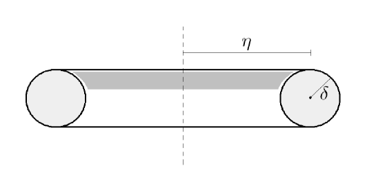
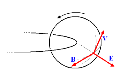
Figure 1: Displacement of the left-handed triplet $({\bf E},{\bf B},{\bf V})$ in the case of a vortex ring. Stationary electromagnetic fields are overlapped to oscillating ones, resulting in a rotation around the major circumference. The first ones provide for charge and magnetic momentum, the second ones are responsible for the curvature of the space and the stability of the configuration.

The cylinder $\Sigma$ is unbounded, so that the energy of our wave turns out to be infinite. We can however build more physical solutions, by imposing that $\Sigma$ is a toroid with major diameter $\eta$ and minor diameter $\delta$ (see figure 1). The stability of vortex rings, from the fluid dynamical point of view, is impressive. We expect the same to happen to our solutions, although, due to the difficulty of the problem, such an analysis looks very hard. The numerical results in [8], show that it is possible to build electromagnetic waves constrained in toroid structures, ranging from the case of a classical ring to a spherical Hill’s type vortex, where the inner hole of the ring is reduced to a segment. The investigation could help us to understand some electric phenomena, such as ball lightning or other self-organized plasmas (see for instance [5]). For the usual ring, the study in [8] indicates that, for $\eta$ slightly bigger than $\delta$, the section $\Omega$ of the toroid is practically a circle. Thus, one may consider solutions where the electric field belongs to the vertical section of the ring, and the magnetic field circulates around the axis (see figure 1). Hence, in good approximation, the expression of the fields can be taken equal to that just obtained for the case of the cylinder. With this setting, we carry out some computations in the coming section, with the aim to illustrate quantitatively that electrons could be modelled by electromagnetic vortex rings of the right size, charge and mass.

6 A model for the electron

The idea that matter at atomic level has a structure recalling that of vortex rings dates back to [25]. At that time, however, the knowledge of atomic physics was very poor. Based on the Maxwell’s model, a first effort to describe a spherical electron with the help of electromagnetic fields was developed in [23] (see also [17]). The project could not be realized due to the scarce information available, both theoretical and experimental. For instance, the concept of spin was not yet introduced. Moreover, general relativity was developed only ten years later, and this, to our opinion, must be a fundamental ingredient for the construction and the stability of the model. Successively, a purely geometrical approach was considered in [26], with the introduction of the so called geons, that is toroid structures in a suitable space-time, roughly approximated by black holes through the Kerr-Newman metric (for more recent results, see [2]). The literature has many other scattered contributions on the subject. In the end, all the proposed models are a bit rough and do not take into account all the features of a particle. Nevertheless, since now we exactly know what a photon is, additional elements are available for a deeper investigation, and the solution we are going to show will be realistic in all the aspects.

Let us consider figure 1. The volume of $\Sigma$ is $2\pi^{2}\eta\delta^{2}$, therefore, the total charge is given by the integral of $\rho={\rm div}{\bf E}$ over $\Sigma$:

$$q~{}=~{}\epsilon_{0}\int_{\Sigma}\frac{2\gamma_{0}}{\omega}~{}=~{}\frac{4\pi^{2}\epsilon_{0}\eta\delta^{2}}{\omega}\gamma_{0}$$ (53)

Thus, we deduce:

$$\gamma_{0}~{}=~{}\frac{q\omega}{4\pi^{2}\epsilon_{0}\eta\delta^{2}}=~{}\frac{q\omega^{3}}{4\pi^{2}\epsilon_{0}\eta\delta_{k}^{2}}$$ (54)

where $\delta=\delta_{k}/\omega$, $\delta_{k}$ being the first zero of $J_{k}$. Successively, by integrating the pressure on $\Sigma$, we obtain:

$$\int_{\Sigma}p~{}=~{}2\pi\eta\int_{\Omega}\left[p_{0}+\frac{c^{2}\omega\gamma_{0}r^{2}}{k^{2}}-\frac{\mu\gamma_{0}^{2}r^{2}}{\omega^{2}}\Big{(}1-\frac{\omega^{2}r^{2}}{2k^{2}}\Big{)}\right]r~{}drd\phi$$ (55)

where $\Omega$ is the circle of radius $\delta=\delta_{k}/\omega$, and we used the stationary part of the expression in (51) (note that the dynamical part has zero average in $\Omega$). Proceeding with the computation we get:

$$\int_{\Sigma}p~{}=~{}4\pi^{2}\eta\left[\frac{p_{0}r^{2}}{2}+\frac{c^{2}\omega\gamma_{0}r^{4}}{4k^{2}}~{}-~{}\frac{\mu\gamma_{0}^{2}r^{4}}{4\omega^{2}}~{}+~{}\frac{\mu\gamma_{0}^{2}r^{6}}{12k^{2}}\right]_{0}^{\delta_{k}/\omega}$$

$$~{}=~{}\frac{2\pi^{2}\eta p_{0}\delta_{k}^{2}}{\omega^{2}}+\frac{\pi^{2}\eta\gamma_{0}\delta^{4}_{k}}{\omega^{3}}\left(\frac{c^{2}}{k^{2}}~{}-~{}\frac{\mu\gamma_{0}}{\omega^{3}}~{}+~{}\frac{\mu\gamma_{0}A_{k}}{3\omega^{3}}\right)$$

$$~{}=~{}\frac{2\pi^{2}\eta p_{0}\delta_{k}^{2}}{\omega^{2}}+\frac{c^{2}qA_{k}}{4\epsilon_{0}}~{}+~{}\frac{\mu q^{2}}{16\pi^{2}\epsilon_{0}^{2}\eta}\left(\frac{A_{k}}{3}-1\right)$$ (56)

where we used (54) and we set $A_{k}=\delta_{k}^{2}/k^{2}$. For convenience, we report in table 1 the values of $\delta_{k}$ and $A_{k}$, for various $k$.

$$\begin{array}[]{|c|c|c|c|}\hline\cr\hskip 2.84544pt~{}k{}&~{}~{}~{}~{}~{}\delta_{k}{}{}{}{}{}&~{}~{}\delta_{k}/k{}{}&~{}A_{k}=\delta_{k}^{2}/k^{2}{}\\ \hline\cr 2&5.1356&2.567&6.593\\ 3&6.3802&2.126&4.522\\ 4&7.5883&1.897&3.598\\ 5&8.7715&1.754&3.077\\ 6&9.9361&1.656&2.742\\ 7&11.086&1.583&2.508\\ 8&12.225&1.528&2.335\\ 9&13.354&1.483&2.201\\ 10&14.476&1.447&2.095\\ 11&15.590&1.417&2.008\\ 12&16.698&1.391&1.936\\ 13&17.801&1.369&1.875\\ 14&18.900&1.350&1.822\\ \hline\cr\end{array}$$

Table 1: Values of $\delta_{k}$ and associated quantities for various $k$.

After recalling the definition (46), we now require that $\rho_{m}=0$ for $r=0$ (zero mass density at the center of the body, in part justified by the fact that $p$ is quadratical with respect to $r$ near the origin). This implies that the constant $p_{0}$ has to be equal to: $c^{2}\rho=2\gamma_{0}c^{2}/\omega$. We also remark that a pure rotating wave with $\gamma_{0}=0$ and $\gamma_{1}\not=0$ (see (50)) turns out to have $m=\int_{\Sigma}\rho_{m}=0$ (since $\rho=0$ and $p=0$), according to the fact that a photon is uncharged and massless, even if it is constrained in a bounded region of space.

Finally, concerning the mass of our toroid, we can write:

$$m~{}=~{}\frac{\epsilon_{0}}{\mu}\int_{\Sigma}\left(\rho-\frac{p}{c^{2}}\right)~{}=~{}-~{}\frac{qA_{k}}{4\mu}~{}-~{}\frac{q^{2}}{16\pi^{2}\epsilon_{0}\eta c^{2}}\left(\frac{A_{k}}{3}-1\right)$$ (57)

Let us assume that $2\leq k\leq 5$, so that $A_{k}>3$ (see table 1). If $q$ is positive, the above expression is certainly negative and cannot represent a mass. If instead $q=-e$ is the electron charge, we have chances to get something interesting. In such a situation, the last expression takes the form:

$$m~{}=~{}\frac{A_{k}}{4}~{}\frac{e}{\mu}~{}-~{}\left(\frac{A_{k}}{3}-1\right)\frac{\alpha h}{8\pi^{2}\eta c}$$ (58)

where $\alpha=e^{2}/2hc\epsilon_{0}$ is the fine structure constant and $h$ is the Planck constant. It is important to observe that $m$ does not depend on $\omega$ and $\delta$ (we discuss this aspect later).

Successively, we may try to find the major diameter $\eta$. As an extra condition, we impose that the radial component of $\nabla p$ is zero at the boundary of $\Omega$. In fact, assuming that $p$ is a kind of gravitational potential (see the end of section 4), this means that no other external forces are pushing on the boundary (except for those related to the centripetal acceleration and the unbalanced Lorentz condition ${\bf E}+{\bf V}\times{\bf B}\not=0$), producing a sort of equilibrium at the surface of $\Sigma$. Thus, in order to determine $\eta$, we set to zero the first relation in (52), at the point $\delta_{k}/\omega$. Considering that $J_{k}(\delta_{k})=0$, we get the relation:

$$\frac{c^{2}}{k^{2}}~{}=~{}\frac{\mu\gamma_{0}}{\omega^{3}}(1-A_{k})$$ (59)

Substituting in (59) the expression of $\gamma_{0}$ given in (54) and introducing the constant $\alpha$, one obtains:

$$\eta~{}=~{}\frac{\mu}{e}\frac{\alpha h}{2\pi^{2}c}\Big{(}1-\frac{1}{A_{k}}\Big{)}$$ (60)

We can go back to (58). With the new value of $\eta$, we can finally write:

$$m~{}=~{}\frac{e}{\mu}~{}\frac{A_{k}^{2}}{6(A_{k}-1)}$$ (61)

Let us discuss the case $k=2$. Assuming to know the values of $e$ and $m$, from (61), we deduce the estimate:

$$\mu~{}=~{}1.295~{}\frac{e}{m}~{}\approx~{}2.27\times 10^{11}~{}{\rm Coulomb/Kg}$$ (62)

A similar estimate of the constant $\mu$ was recovered in [11] by different arguments. Successively, from (60) we can compute $\eta$:

$$\eta~{}=~{}\frac{\alpha hA_{k}}{12\pi^{2}mc}~{}\approx~{}.985~{}\times 10^{-15}~{}{\rm meters}$$ (63)

that agrees quite well with the Compton radius of an electron.

Let us see what happens to the electromagnetic energy. We take the stationary parts of the fields in (50). With computations similar to those carried out above, we can evaluate the energy:

$${\cal E}~{}=~{}\frac{\epsilon_{0}}{2}\int_{\Sigma}(|{\bf E}|^{2}+c^{2}|{\bf B}|^{2})$$

$$=~{}\pi\epsilon_{0}\eta\int_{\Omega}\left[\Big{(}\frac{\gamma_{0}r}{\omega}\Big{)}^{2}+\Big{(}\frac{\gamma_{0}r^{2}}{k}\Big{)}^{2}\right]~{}=~{}\Big{(}1+\frac{2A_{k}}{3}\Big{)}~{}\frac{\alpha hc}{16\pi^{2}\eta}$$ (64)

For $k=2$, using the values already computed, we arrive at:

$${\cal E}~{}=~{}\frac{1}{2}\Big{(}1+\frac{3}{2A_{k}}\Big{)}mc^{2}~{}\approx~{}.614~{}mc^{2}$$ (65)

The remaining part of the energy may be provided by the dynamical part. At this point, one computes $\gamma_{1}$ in (50), in order to get a total energy corresponding to $~{}mc^{2}=(\epsilon_{0}/\mu)\int_{\Sigma}(\rho c^{2}-p)$, that, written in this form, takes the meaning of a potential energy (recall that $\rho$ is constant in $\Sigma$).

By analyzing $g_{00}$ in (44), we can get further information. For example, if the radius $\eta$ of the particle coincides with the horizon, so that $(Q/\eta)^{2}\approx 1$, one should have: $\chi\approx 32(\pi c^{2}\eta\epsilon_{0}/\mu e)^{2}\approx 0.145$.

In the end, we were able to prove the following facts. It is possible to build electromagnetic vortex rings having the size ($2\eta$), the charge ($-e$) and the mass ($m$) of an electron (see also [6]). Note that some computations could have been made in a different way. For instance, in the definition of $\rho_{m}$ (see (46)), we can include a further multiplicative adimensional constant. The aim was however to show that there exists at least an admissible setting.

Since our particles are made of rotating photons, it is natural to associate an intrinsic spin to them, even if they are not mechanically rotating around an axis. There is also a magnetic field inside the toroid, having zero dipole moment. This implies that the particle is ‘neutral’ from the magnetic viewpoint, but, under external solicitations, it may exhibit a magnetic momentum. The triplet $({\bf E},{\bf B},{\bf V})$ is left-handed and this has something to do with the concept of chirality. In fact, the specular image of our particle, obtained by switching the sign of the charge, produces an anti-particle (the positron), sharing the same properties of the electron, as it can be proven with similar computations (compare (20) and (31)). When an electron and a positron collide, they destroy their stable geometrical environment, producing pure photons departing from the impact site according to standard mechanical rules.

There is no a single solution, but a multitude of them, depending on the parameter $\omega$. As a matter of fact, maintaining the amplitude of $\eta$, we can construct thin rings $\Sigma$ having the sections $\Omega$ rotating at very fast speed. Their charge and mass densities are high and the volume small. Conversely, one can build fat rings with lower angular velocity. Probably, there exists an intermediate solution optimizing the energy, but, with an analysis at the first order, we were not able to detect it. Thus, we can associate to our particle infinite frequencies. However, the whole object has a fixed global diameter $2\eta$, that can be formally taken as the wave-length of a suitable fictitious internal clock (see for instance [15]). These facts are not disturbing however. They make the electron a very adaptable particle when interacting with the outside world, explaining why it can emit photons with a continuous spectrum and escape to finer measurements. In order to justify these assertions, one has to assume that the bare particle is ‘dressed up’ with a cloud of photons, bringing different frequencies and responsible for the transmission of the electric charge to the environment. At this point, the discussion becomes more delicate and the interested reader is addressed to [11], chapter 6, and [12], where the author gives his personal interpretation on issues regarding the quantization of matter.

Switching the sign of both the electric and magnetic fields, should bring to a positive left-handed particle. Its structure is going to be quantitatively different from that of the electron, since the forces in (24) find their balance in an alternative way. We do not think however that the standard ring will be stable in this case, while we guess that a Hill’s type vortex would be more appropriate (see [8]). On the other hand, if also protons can be described by our model, we do expect they assume complicated shapes (see [21]) and display peculiar substructures, as it is revealed by experiments.

References

- [1] Aldrovandi R., Pereira J. G., Vu K. H. (2007), The nonlinear essence of gravitational waves, Found. Phys., 37, pp. 1503-1517.
- [2] Arcos H. I., Pereira J. C. (2004), Kerr-Newman solution as a Dirac particle, Gen. Rel. Grav., 36, n. 11, pp. 2441-2464.
- [3] Atwater H. A. (1974), Introduction to General Relativity, Pergamon Press, Oxford.
- [4] Bondi H., Pirani F. A. E., Robinson I. (1959), Gravitational waves in general relativity, III, Exact plane waves, Proc. R. Soc. Lond. A, 251, pp. 519-533.
- [5] Chen C., Pakter R., Seward D. C. (2001), Equilibrium ans stability properties of self-organized spiral toroids, Physics of Plasmas, 8, n. 10, pp. 4441-4449.
- [6] Cernitskii A. A. (2006), Mass, spin, charge, and magnetic moment for electromagnetic particle, arXiv: hep-th/0603040v1
- [7] Cernitskii A. A. (2009), On unification of gravitational and electromagnetism in the framework of a general-relativistic approach, arXiv: gr-qc/0907.2114v1
- [8] Chinosi C., Della Croce L., Funaro D. (2009), Rotating electromagnetic waves in toroid-shaped regions, to appear in Int. J. of Modern Phys. C.
- [9] Dirac P. A. M. (1928), The quantum theory of the electron, Proc. Roy. Soc., London, A 117, pp. 610-624.
- [10] Fock V. (1959), The Theory of Space Time and Gravitation, Pergamon Press, London.
- [11] Funaro D. (2008), Electromagnetism and the Structure of Matter, World Scientific, Singapore.
- [12] Funaro D. (2009), The fractal structure of matter and the Casimir effect, arXiv: 0906.1874v1
- [13] Funaro D. (2009), Numerical simulation of electromagnetic solitons and their interaction with matter, J. Sci. Comput., DOI 10.1007/s10915-009-9338-5
- [14] Funaro D., A model for electromagnetic solitary waves in vacuum, submitted to Mathematics and Computers in Simulations.
- [15] Gouanère M. et al. (2005), Experimental observation compatible with the particle internal clock, Annales de la Fondation L. de Broglie, 30, n. 1, pp. 109-114.
- [16] Landau L. D., Lifshitz E. M. (1962), The Classical Theory of Fields, Pergamon Press, Warsaw.
- [17] Levi-Civita T. (1907-8), Sui campi elettromagnetici puri dovuti a moti piani permanenti, Atti Ist. Veneto, LXVII, Parte II, pp. 995-1010.
- [18] Lo C. Y. (2006), The gravity of photons and the necessary rectification of Einstein equation, Progress in Physics, 1, pp. 46-51.
- [19] Maxwell J. C. (1861), On physical lines of forces, The London, Edinburgh and Dublin Philosophical Magazine and Journal of Science.
- [20] Maxwell J. C. (1865), A dynamical theory of electromagnetic fields, Philosophical Transactions of the Royal Society of London, 155, pp. 459-512.
- [21] Miller G. A. (2003), Shapes of the proton, Phys. Rev. C, 68, 022201(R).
- [22] Misner C. W., Thorne K. S., Wheeler J. A. (1973), Gravitation, W. H. Freeman & c., San Francisco.
- [23] Poincaré M. H. (1906), Sur la dynamique de l’électron, Rend. Circ. Palermo, XXI, pp. 129-175.
- [24] Rizzi G, Ruggiero M. L., Eds. (2004), Relativity in Rotating Frames, Kluwer Academic, The Netherlands.
- [25] Thomson W. (Lord Kelvin) (1867), On vortex atoms, Proceedings of the Royal Society of Edinburgh, VI, pp. 94-105.
- [26] Wheeler J. A. (1955), Geons, Phys. Rev., 97, n. 2, pp. 511-536.