Polarization-correlated photon pairs from a single ion

Abstract

In the fluorescence light of a single atom, the probability for emission of a photon with certain polarization depends on the polarization of the photon emitted immediately before it. Here correlations of such kind are investigated with a single trapped calcium ion by means of second order correlation functions. A theoretical model is developed and fitted to the experimental data, which show 91% probability for the emission of polarization-correlated photon pairs within 24 ns.

I Introduction

One of the most relevant tools for characterizing the light field emitted by a quantum optical system is its intensity correlation function $g^{(2)}(\tau)$, the most prominent example being the observation of antibunching Kimble1977PRLv39p691 ; Diedrich1987PRLv58p203 in the fluorescence of a single atom. Intensity correlation functions of the fluorescence light of a single ion excited by two light fields have been investigated before. In Schubert1992PRLv68p3016 the pair correlation conditioned on the wavelength of the photons scattered by a $\mathrm{Ba^{+}}$ ion (eight-level structure) reveal the transient internal dynamics of the ion, which is characterized by optical pumping and the excitation of Raman coherence. In a detailed description of these experiments Schubert1995PRAv52p2994 , it is shown that measuring the correlation function for only one polarization of one of the two light fields by adding a polarization filter projects the ion in a coherent superposition of its energy eigenstates. This may be considered a first signature of atom-photon entanglement PET .

Other investigations of the resonance fluorescence of coherently driven single atoms by means of $g^{(2)}(\tau)$ comprise, e.g., a theoretical analysis of the effect of the quantized motion of a two-level atom in a harmonic trap on the second order correlation function Jakob1999PRAv59p2111 , experimental measurements of photon correlations revealing single-atom dynamics in a magneto-otical trap Gomer1998PRAv58p1657 ; Gomer1998APBv67p689 and atomic transport in an optical lattice Jurczak1996PRLv77p1727 , the theoretical demonstration of nonclassical correlations in the radiation of two atoms Skornia2001PRAv64p63801 , i.e. bunched and anti-bunched light is emitted in different spatial directions, and the study of intensity-intensity correlations from a three-level atom damped by a broadband squeezed vacuum Carreno2004JoOBv6p315 .

Another application of photon-photon correlations in the resonance fluorescence from single atoms is an experiment where, using a self homodyning configuration, the second order correlation function was used to characterize the secular motion of a trapped ion Rotter2008NJPv10p43011 . The experiment revealed the dynamics of both internal and external degrees of freedom of the ion’s wave function, from nanosecond to millisecond timescales, in a single measurement run.

Polarization correlations of subsequent photons enitted from a bichromatically driven four-level atom have been predicted theoretically Jakob2002JOBv4p308 . In this proposal a four-level atom ($\mathrm{J=1/2}$ to $\mathrm{J=1/2}$) with degenerate Zeeman sub-states is coupled to a light field consisting of two components which are symmetrically detuned from the resonance frequency of the atomic transition. In contrast, in the experiment presented in this paper, the Zeeman degeneracy is lifted and the corresponding atomic transition (four-level system) is driven monochromatically. Furthermore, the effect of the coupling of the excited states to another manifold ($\mathrm{J=3/2}$) of four Zeeman sub-levels by a second light field is taken into account.

In the context of quantum optical information technologies, many entanglement protocols strongly rely on a projective measurement Cabrillo1999PRAv59p1025 ; Browne2003PRLv91p67901 ; Feng2003PRLv90p217902 ; Duan2003PRLv90p253601 ; Simon2003PRLv91p110405 , which is also the origin of the effect of antibunching. In fact, the degree of antibunching is a benchmark for single quantum emitters or ideal single photon sources that are suitable for quantum networking and communication.

Beyond proving that a source is a pure single quantum emitter, correlation functions are used to characterize and develop applications for quantum communication. In Dubin2007PRLv99p183001 , for example, the resonance fluorescence from a continuously excited single ion is split and recombined on a beam splitter with a relative delay, thus creating an effective two-photon source. Here the measured correlation function reveals the quality of the mode matching at the beam splitter. Measuring and controlling the degree of second order correlation of a photon source is therefore a very important step in designing quantum optical tools in quantum information processing. This engineering of correlation functions is of special interest for quantum networks where single photons mediate information between nodes of single atoms Zoller2005EPJDv36p203 ; Briegel1998PRLv81p5932 .

In this context, we present a polarization selective measurement of the correlation function $g^{(2)}(\tau)$ of fluorescence photons from a single ${}^{40}\mathrm{Ca^{+}}$ ion, which is continuously laser excited on the $\mathrm{4^{2}S_{1/2}}$ to $\mathrm{4^{2}P_{1/2}}$ transition. In particular, the correlation function of emitted $\sigma^{-}$ and $\sigma^{+}$ polarized photons was measured conditioned on the previous detection of a $\sigma^{-}$ photon, and it is shown that the system can be tailored such that the polarization of a photon depends strongly on the polarization of a previous one.

II Model

Figure 1 shows the relevant levels of the ${}^{40}\mathrm{Ca^{+}}$ ion. Continuous excitation with laser light at 397 nm and 866 nm generates continuous resonance fluorescence. We consider the case of observation along the direction of the magnetic field and write $g^{(2)}(\tau)$ in terms of the transition operators for the $\sigma$-transitions from $\mathrm{S_{1/2}}$ to $\mathrm{P_{1/2}}$ (see figure 1 for the numbering of the levels),

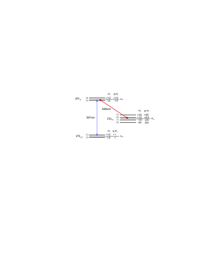
Figure 1: Level scheme of $\mathrm{{}^{40}Ca^{+}}$ for a non zero magnetic field $\vec{\mathrm{B}}$. The $\mathrm{{}^{2}S_{1/2}}$, $\mathrm{{}^{2}P_{1/2}}$ and $\mathrm{{}^{2}D_{3/2}}$ states split into eight levels according to their magnetic quantum number $m_{j}$ and the Landé factors $g_{j}$. The splitting shown is not to scale.

$$\hat{\sigma}_{1} = |1\rangle\langle 4|,\hskip 28.45274pt\hat{\sigma}_{1}^{\dagger}=|4\rangle\langle 1|,$$ (1)

$$\hat{\sigma}_{2} = |2\rangle\langle 3|,\hskip 28.45274pt\hat{\sigma}_{2}^{\dagger}=|3\rangle\langle 2|.$$ (2)

If we consider the general case without polarization selective detection, the second order correlation function reads Loudon2000

$$g^{(2)}(\tau)=\frac{\sum_{i,j=1}^{2}\langle\hat{\sigma}^{\dagger}_{i}(t)\hat{\sigma}^{\dagger}_{j}(t+\tau)\hat{\sigma}_{j}(t+\tau)\hat{\sigma}_{i}(t)\rangle}{\langle\hat{\sigma}^{\dagger}_{1}(t)\hat{\sigma}_{1}(t)+\hat{\sigma}^{\dagger}_{2}(t)\hat{\sigma}_{2}(t)\rangle^{2}}.$$ (3)

Using the quantum regression theorem Mandel1995 it can be shown that for all initial conditions and at steady state, the second order correlation function is related to the excited state populations by

$$g^{(2)}(\tau)=\frac{\rho_{33}(\tau)+\rho_{44}(\tau)}{\rho_{33}(\infty)+\rho_{44}(\infty)},$$ (4)

where $\rho_{lm}(\tau)$ with $l,m\in[1,8]$ are the matrix elements of the density operator representing populations and coherences of the states $|l\rangle$ and $|m\rangle$ at time $\tau$ after the detection of a first photon. Equation 4 allows to predict $g^{(2)}$ by solving the optical Bloch equations. The second order correlation function $g^{(2)}(\tau)$ of the 397 nm fluorescence light of a single ${}^{40}\mathrm{Ca^{+}}$ ion is thus proportional to the population of the ion’s excited state $\mathrm{P_{1/2}}$ at time $\tau$ whereby the initial state at $\tau=0$ is determined by the first measured photon.

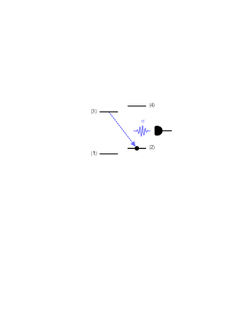
(a) Projection

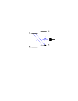
(b) $\sigma^{-}$ polarized photon

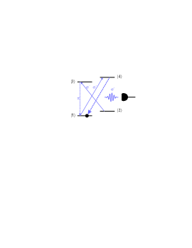
(c) $\sigma^{+}$ polarized photon

Figure 2: Detection of $\sigma^{-}$ (b) and $\sigma^{+}$ (c) polarized photons, conditioned on the previous detection of a $\sigma^{-}$ (a) polarized photon. Excitation happens with $\sigma^{+}$-$\sigma^{-}$-polarized light, i.e. linear polarization perpendicular to the magnetic field. (a) Detection of a $\sigma^{-}$ polarized photon projects the ion into the state $|2\rangle=|S_{1/2},m_{j}=1/2\rangle$. (b) To detect a subsequent $\sigma^{-}$ polarized photon, the ion has to be re-excited under the absorption of a $\sigma^{-}$ polarized photon. (c) To detect a $\sigma^{+}$ polarized photon, the ion has to be re-excited under the absorption of a $\sigma^{-}$ polarized photon, then decay to state $|1\rangle$ under emission of a $\pi$ polarized photon and then be excited to the state $|4\rangle$ by reabsorbing a $\sigma^{+}$ polarized photon from the exciting beams.

We now consider polarization-selective detection of photons for the situation of our experiment. Figure 2 shows a sketch of the four levels involved in the emission of blue (397 nm) photons on the $\mathrm{P_{1/2}}$ to $\mathrm{S_{1/2}}$ transition. The detection of a $\sigma^{-}$ polarized photon projects the ion into state $|2\rangle=|\textrm{S}_{1/2},m_{j}=1/2\rangle$ (figure 2a). If the ion is continuously illuminated by linearly polarized light at 397 and 866 nm with polarization perpendicular to the magnetic field, no $\pi$ transitions are excited. The ion effectively sees a superposition of $\sigma^{-}$ and $\sigma^{+}$ polarized light. After the emission of a $\sigma^{-}$ photon and the corresponding projection into state $|2\rangle$, a subsequent excitation can thus only occur to state $|3\rangle=|\textrm{P}_{1/2},m_{j}=-1/2\rangle$ by absorbing a $\sigma^{-}$ polarized photon. From state $|3\rangle$ the ion can either decay back to state $|2\rangle$ under emission of a second $\sigma^{-}$ polarized photon (figure 2b), or it can decay to state $|1\rangle=|\textrm{S}_{1/2},m_{j}=-1/2\rangle$ under emission of a $\pi$ polarized photon. Thus the next emitted photon after a $\sigma^{-}$ photon can not be $\sigma^{+}$ polarized. In order to emit a $\sigma^{+}$ polarized photon, the ion must first be excited to state $|4\rangle=|\textrm{P}_{1/2},m_{j}=1/2\rangle$, which can only happen out of state $|1\rangle$ by absorbing a $\sigma^{+}$ polarized photon from the exciting beams (figure 2c). The probability of detecting a $\sigma^{+}$ polarized photon after the time $\tau$ conditioned on the previous detection of a $\sigma^{-}$ polarized photon is therefore much lower than the probability of detecting a $\sigma^{-}$ polarized photon for the same condition. Since the correlation function is a measure for the photon-photon waiting time distribution, the $g^{(2)}$ derived from correlating $\sigma^{-}$ with $\sigma^{+}$ photons should be suppressed with respect to the $g^{(2)}$ derived from correlating $\sigma^{-}$ with $\sigma^{-}$ photons. In fact both correlations are expected to exhibit almost ideal antibunching, with the difference that for the first case the dip around $\tau$=0 is expected to be much wider. In other words, and taking into account also the case where $\sigma^{+}$ and $\sigma^{-}$ are exchanged, there will be a much stronger antibunching for the correlation of photons with opposite $\sigma$ polarization than for photons with the same $\sigma$ polarization. The same considerations are applicable for excitation with pure $\pi$-polarized light. In that case the correlation of subsequent photons is much stronger for opposite than for equal $\sigma$ polarization.

Analogous to equation 4, the second order correlation functions for $\sigma^{-}$ and $\sigma^{+}$ light, conditioned on the previous detection of a $\sigma^{-}$ photon ($\hat{\rho}(0)=\hat{\rho}_{\mathrm{init}}=|2\rangle\langle 2|$) are derived to be

$$g^{(2)}_{\sigma^{-}}(\tau)=\frac{\rho_{33}(\tau)}{\rho_{33}(\infty)}$$ (5)

and

$$g^{(2)}_{\sigma^{+}}(\tau)=\frac{\rho_{44}(\tau)}{\rho_{44}(\infty)},$$ (6)

respectively. In contrast to the general case (equation 4) the conditioned second order correlation function is given by only one of the excited state populations at time $\tau$.

In figure 3a and 4a the correlation functions calculated according to equations 5 and 6 are plotted for weak and strong excitation parameters typical for our experimental setup. The upper curves, in blue, show $g^{(2)}_{\sigma^{-}}(\tau)$, while the lower ones, in red, represent $g^{(2)}_{\sigma^{+}}(\tau)$. As expected $g^{(2)}_{\sigma^{-}}(\tau)$ and $g^{(2)}_{\sigma^{+}}(\tau)$ show very different behaviors. For both weak and strong excitation, $g^{(2)}_{\sigma^{-}}(\tau)$ rises to high values with a steep slope. For weak excitation a maximum $g^{(2)}$ of 15.6 is reached at $\tau=\pm 29\,\mathrm{ns}$. For longer time differences the correlation function falls monotonously until it reaches one. For strong excitation $g^{(2)}_{\sigma^{-}}(\tau)$ reaches a maximal value of 2.8 at $\tau=\pm 13\,\mathrm{ns}$. For $\tau>13\,\mathrm{ns}$ the correlation function falls to 1 after 200 ns showing some coherent oscillations.

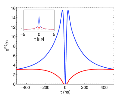
(a)

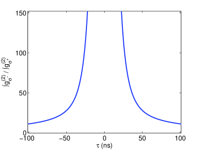
(b)

Figure 3: (a) Conditioned second order correlation functions $g^{(2)}_{\sigma^{-}}(\tau)$ (top, blue) and $g^{(2)}_{\sigma^{+}}(\tau)$ (bottom, red) for weak excitation. The functions have been calculated with a eight level Bloch equation model for Rabi frequencies of $\Omega_{397}=2\pi\cdot 9.2\,\mathrm{MHz}$, $\Omega_{866}=2\pi\cdot 1.3\,\mathrm{MHz}$, detunings $\Delta_{397}/2\pi=-15\,\mathrm{MHz}$, $\Delta_{866}/2\pi=5.8\,\mathrm{MHz}$ and a magnetic field of $\mathrm{B}=3.5\,\mathrm{G}$. (b) Ratio $p(\tau)$ (equation 7) of the integrals over time of the two conditioned correlation functions.

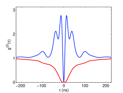
(a)

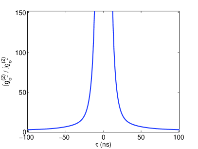
(b)

Figure 4: (a) Conditioned second order correlation functions $g^{(2)}_{\sigma^{-}}(\tau)$ (top, blue) and $g^{(2)}_{\sigma^{+}}(\tau)$ (bottom, red) for strong excitation. The functions have been calculated with a eight level Bloch equation model for Rabi frequencies of $\Omega_{397}=2\pi\cdot 20.2\,\mathrm{MHz}$, $\Omega_{866}=2\pi\cdot 20.3\,\mathrm{MHz}$, detunings $\Delta_{397}/2\pi=-15\,\mathrm{MHz}$, $\Delta_{866}/2\pi=5.8\,\mathrm{MHz}$ and a magnetic field of $\mathrm{B}=3.5\,\mathrm{G}$. (b) Ratio $p(\tau)$ (equation 7) of the integrals over time of the two conditioned correlation functions.

The two $g^{(2)}_{\sigma^{+}}(\tau)$ functions, on the contrary, show a flat behavior on short time scales before they rise with a moderate slope to their maximum value, which is reached at approximately 400 ns for the weak excitation and 200 ns for the strong excitation. In the latter case $g^{(2)}_{\sigma^{+}}(\tau)$ rises directly to 1 without a transient overshoot, while for weak excitation it reaches a value of 3.1 before it falls to 1 for $\tau>400\,\mathrm{ns}$.

The shape of $g^{(2)}_{\sigma^{-}}(\tau)$ in figure 3a is characterized by large correlation values and a long decay time (compared to the lifetime of the $\mathrm{P_{1/2}}$ state) to the asymptotic value and can be attributed to optical pumping into the $\mathrm{D_{3/2}}$ state Schubert1995PRAv52p2994 . The excitation on the $\mathrm{S_{1/2}-P_{1/2}}$ transitions is much stronger than the one on the $\mathrm{D_{3/2}-P_{1/2}}$ transitions. As a result, a large fraction of the population is transferred to the $\mathrm{D_{3/2}}$ state after long delay times and the observed fluorescence is weak. This small flux of fluorescence, caused by a small steady-state population of the state $|3\rangle$, determines the normalization factor for long time intervals $\rho_{33}(\infty)$. At short time delays after the projection into state $|2\rangle$, however, i.e. during the first 30-40 ns, a large fraction of the population is excited to state $|3\rangle$ and the optical pumping to the $\mathrm{D_{3/2}}$ states is negligible. Since the correlation function is the ratio of the population of state $|3\rangle$ at time $\tau$ and that in the steady state, high values are reached, which then decay to one revealing the time scale of the optical pumping.

The characteristics of $g^{(2)}_{\sigma^{+}}(\tau)$ can be explained with an analogous argumentation. Here, excitation to state $|4\rangle$ during the first 30-40 ns is even smaller than the steady state population $\rho_{44}(\infty)$ for long time delays. After the projection into $|2\rangle$, it takes several scattering events and therefore more time until the population of state $|4\rangle$ exceeds $\rho_{44}(\infty)$. As the inset of figure 3a shows, for large time intervals $g^{(2)}_{\sigma^{+}}(\tau)$ decays to the asymptotic value with the same time constant as $g^{(2)}_{\sigma^{-}}(\tau)$.

The correlation functions shown in figure 4a are calculated for equal excitation strength on the $\mathrm{S_{1/2}-P_{1/2}}$ and $\mathrm{D_{3/2}-P_{1/2}}$ transitions. Consequently, the correlation values of $g^{(2)}_{\sigma^{-}}(\tau)$ are smaller and the decay to the asymptotic value is much faster. The exciting fields are strong enough to cause some damped oscillations at the generalized Rabi frequency $\Omega_{G}=\sqrt{|\Omega_{397}|^{2}+\Delta_{397}^{2}}$ in the correlation function. Due to the complex eight-level structure, the oscillations do not occur at only one generalized Rabi frequency, but each transition between the Zeeman sub-levels contributes a Fourier component depending on the intensity and detuning of the driving field. In figure 4a this becomes noticeable by comparing the frequency of the strongly suppressed oscillations of $g^{(2)}_{\sigma^{+}}(\tau)$ with the ones from $g^{(2)}_{\sigma^{-}}(\tau)$. Due to the Zeeman splitting, the detunings of the $|1\rangle$ to $|4\rangle$ and the $|2\rangle$ to $|3\rangle$ transitions with respect to the exciting laser give rise to different generalized Rabi frequencies.

The most interesting feature in figure 3a and 4a is the behavior of the correlation function for times $\tau$ close to zero. $g^{(2)}_{\sigma^{+}}(\tau)$ shows a flat plateau of values very close to zero for $-15\,\mathrm{ns}<\tau<15\,\mathrm{ns}$ in the case of weak and for $-10\,\mathrm{ns}<\tau<10\,\mathrm{ns}$ in the case of strong excitation. In the same time interval $g^{(2)}_{\sigma^{-}}(\tau)$ rises very fast to high values for both excitation conditions. The ratio

$$p(\tau)=\frac{\int_{0}^{\tau}g^{(2)}_{\sigma^{-}}(t)dt}{\int_{0}^{\tau}g^{(2)}_{\sigma^{+}}(t)dt}$$ (7)

of the number of $\sigma^{-}$- and $\sigma^{+}$-polarized photons emitted by the ion in $\tau$ describes the purity of the polarization in that time window. The probability with which, if a second photon is detected within this time interval, the polarization of this second photon is $\sigma^{-}$, is easily calculated as $\frac{p}{1+p}$. Figure 3b and 4b show $p$ for weak and strong excitation conditions, respectively. The ratio diverges for $\tau\rightarrow 0$ ($>10^{5}$ for $\tau=1\,\mathrm{ns}$) in both excitation regimes, because $\rho_{33}(\tau)$ increases quadratically in time from $\tau=0$, while $\rho_{44}(\tau)$ increases with $\tau^{4}$. In other words, if a second photon is emitted within a short time interval after a first $\sigma^{-}$-polarized photon, then with very high probability (that can be chosen by the time interval) it will also be $\sigma^{-}$-polarized. By exciting the ion with $\pi$-polarized light it is possible to generate equally strongly correlated photon pairs of oppositely $\sigma$-polarized photons.

III Experiment

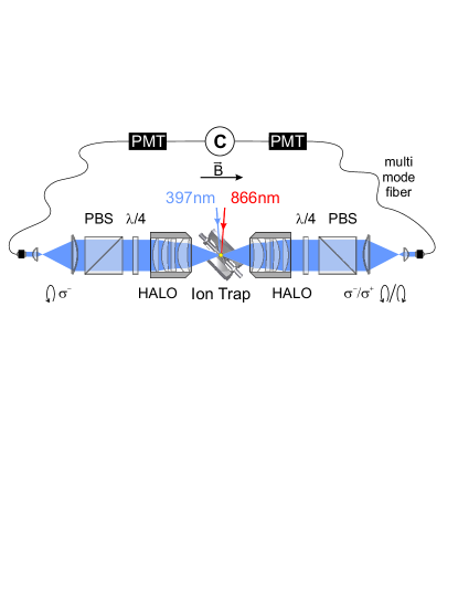
Figure 5: Setup for the measurement of polarization-conditioned correlation functions. The fluorescence light is split in to two parts by collecting it with the two HALO lenses. Multimode fibers are used to couple the light to two PMTs.

Figure 5 shows the setup of the measurement which is described in detail elsewhere Gerber2009NJoPv11p13 ; Rohde2009a[vp . A single ${}^{40}\mathrm{Ca^{+}}$ ion is trapped in a linear Paul trap and continuously excited by two lasers at $397$ nm and $866$ nm. The $397\,\mathrm{nm}$ laser is red detuned to provide Doppler cooling while the resonant $866$ nm laser prevents optical pumping to the $\mathrm{D_{3/2}}$ state. The 397 nm fluorescence light is split into two parts by collecting it with two high numerical aperture lenses (HALO) Gerber2009NJoPv11p13 . Both lenses direct the collected photons to photo multipliers (PMT) through multimode fibers. In each beam path a $\lambda/4$ plate and a polarizing beam splitter are used to select the respective polarization. The arrival times of the signals from the PMTs are recorded with picosecond resolution by commercial counting electronics , and the correlation function is obtained by postprocessing the data.

III.0.1 Calibration

Before measurement of the correlation functions, an excitation spectrum, i.e. the rate of 397 nm fluorescence as a function of the detuning of 866 nm, was recorded. The spectrum that shows four dark resonances provides a calibration of the experimental parameters, which are then used as the starting point to fit the conditioned correlation functions. In figure 6 this excitation spectrum is plotted.

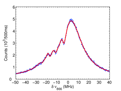
Figure 6: Excitation spectrum of a single ion. The 397 and 866 nm lasers are approximately vertically polarized and propagate under $90^{\circ}$ to the quantization axis (see figure 5). The solid line (red) is the calculated spectrum for the Rabi frequencies $\Omega_{397}=2\pi\cdot 9.9\,\mathrm{MHz}$, $\Omega_{866}=2\pi\cdot 1.5\,\mathrm{MHz}$, the detuning $\Delta_{397}/2\pi=-15\,\mathrm{MHz}$ and a magnetic field of $\mathrm{B}=3.5\,\mathrm{G}$. The background is 89 c.p.s. and the data points shown have Poissonian errors.

The Rabi frequencies, detunings and the magnetic field which are deduced from a fit to the data are indicated in the caption. To account for experimental deviations in the polarization angle of the excitation lasers from the ideal vertical polarization, this parameter was also varied in the fit. The angles of the polarizations of the two laser beams with the magnetic field, as used in the model shown in figure 6, are $\alpha_{397}=0.46\cdot\pi$ for the blue laser and $\alpha_{866}=0.4\cdot\pi$ for the infrared laser (rather than $\pi/2$ in the ideal case). This is compatible with the available control over the experimental settings and the quality of the optical components used.

III.0.2 Conditioned correlation functions

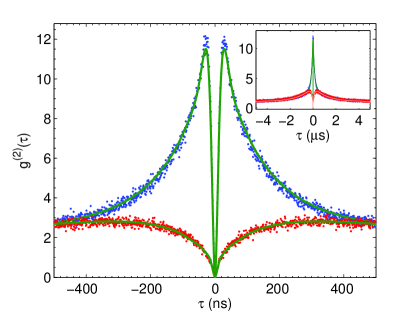
Figure 7: Blue (top): ($g^{(2)}_{\sigma^{-}}$). Red (bottom): ($g^{(2)}_{\sigma^{+}}$). The solid lines (green) are the correlation functions expected from the theoretical model for the Rabi frequencies $\Omega_{397}=2\pi\cdot 9.2\,\mathrm{MHz}$, $\Omega_{866}=2\pi\cdot 1.3\,\mathrm{MHz}$ and the detuning $\Delta_{866}/2\pi=5.8\,\mathrm{MHz}$. The inset shows data and model for time scales up to $5\,\mathrm{\mu s}$.

Figure 7 shows the data for the two measured conditioned correlation functions plotted in one graph. Data for $g^{(2)}_{\sigma^{+}}$ are presented in red (lower curve) and data for $g^{(2)}_{\sigma^{-}}$ in blue (upper curve). The data are normalized to a long-time value of one and presented without background subtraction. The solid lines are the $g^{(2)}$ functions obtained by a fit of the Rabi frequencies to the experimental data using the model discussed in section II. The values of the background, laser detunings, magnetic field as well as the polarization angles extracted from the fit to the excitation spectrum have been kept fixed. The two Rabi frequencies have been fitted to both curves at the same time and agree well with the experiment. The deviation of the Rabi frequencies between the fitted correlation functions and the fitted excitation spectrum lies within the statistical error . The correlation functions are very similar to the ones for the case of weak excitation in figure 3. For large $\tau$ ($>$ 400 ns) both functions overlap and slowly decay to one. The characteristic behavior of large (small) correlation values and the slow decay to the asymptotic value for $g^{(2)}_{\sigma^{-}}$ ($g^{(2)}_{\sigma^{+}}$), explained in section II, are clearly observed in the measurement.

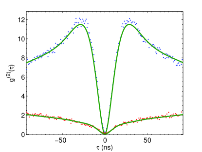
Figure 8: Zoom of FIG. 7

Figure 8 shows a zoom into the region for small time differences. At $\tau=0$ both curves reach a value close to zero. With increasing $\tau$, $g^{(2)}_{\sigma^{-}}$ rises with a very steep quadratic slope and reaches a value as large as 12, whereas $g^{(2)}_{\sigma^{+}}$ stays flat for $\sim 5\,\mathrm{ns}$, before it rises with a moderate slope to a maximum value of 2.9. The model agrees very well with the data, proving the good control over the creation of polarization correlated photon pairs that we obtained experimentally.

The main difference between the model calculation of $g^{(2)}$ in figure 3a and experimental data in figure 8 is that the predicted $\tau^{4}$-like plateau of $g^{(2)}_{\sigma^{+}}(\tau)$ is less pronounced in the measurement. Simulations with the model from section II show that this is explained by small errors in the polarization of the exciting lasers and in the detection setup. The polarizations of the exciting lasers have been fitted to the excitation spectrum (fig 6), and these results have been used in the model of the correlation functions. To achieve an agreement of the quality as it is shown in figure 7 and 8, also deviations from the ideal polarizations in the detection were accounted for in the model. These deviations occur when the polarization is not filtered perfectly, and consequently the measured $g^{(2)}$ function contain some coincidences that are caused by the respective orthogonal polarization. The theoretical model in figures 7 and 8 has been calculated using 2.5 % of wrong $\sigma^{+}$ polarized photons for the initial detection events in both curves. For $g^{(2)}_{\sigma^{-}}$ the conditioned detection of the second $\sigma^{-}$ polarized photon has an error of 5%, while for $g^{(2)}_{\sigma^{+}}$ the detection of the $\sigma^{+}$ polarized photon has an error of 1.8%. This demonstrates that $g^{(2)}_{\sigma^{+}}$, in particular its $\tau^{4}$ characteristic, is very sensitive to small polarization errors at times $\tau$ close to zero. These errors are within the precision with which the polarization filtering was controlled in the experiment, given the low light levels and imperfections of the optics. Furthermore, there is a contribution due to the collection of light from a solid angle along the quantization axis. Each HALO lens collects 4% of the light emitted into the full solid angle Gerber2009NJoPv11p13 , which leads to the detection of a small fraction wrong $\sigma$ and $\pi$ polarized photons.

The sensitivity of the generation of polarization correlated photon pairs to polarization errors gets even more evident considering the purity $p$ (equation 7). Figure 9 shows this ratio for the values of the model calculation that was fitted to the data from figure 7 and 8.

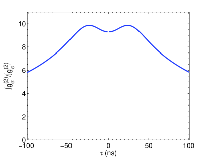
Figure 9: Purity $p$ for the model calculation fitted to the measured data from figure 7 and 8. To avoid artifacts at times close to zero $p$ is presented without background.

In contrast to the ideal case from figure 3b, $p$ does not diverge for times $\tau\rightarrow 0$, but instead reaches a maximum of almost 10 at 24 ns and falls then to 9.3 at 1 ns. This means, if a second photon is detected with our setup within 24 ns, it is $\sigma^{-}$ polarized with 91 % probability. A practical figure of merit also has to consider the absolute number of photons within the time interval $\tau$. After 24 ns the ion emits on average 0.07 $\sigma^{-}$ polarized photons into the full solid angle, out of which 8% are detected with our setup Gerber2009NJoPv11p13 . Increasing the time window will yield more photons, but decrease the polarization purity. The curve for the ideal case in figure 3b reaches a value of 130 at 24 ns, suggesting that it is in principle possible to generate polarization correlated photon pairs with more than 99% probability using this method. This could be achieved by reducing polarization errors in excitation and detection.

The excitation conditions of the single ion also affect the efficiency of our photon pair source. For the strong excitation conditions of figure 4, for example, the ion emits on average 0.2 $\sigma^{-}$ polarized photons within 24 ns. Simultaneously the purity decreases, yielding a $\sigma^{-}$ polarized photon in only 96% of the cases (figure 4b). For a good comparison of the source under weak and strong excitation conditions it is convenient to look at the efficiency of both cases for equal photon numbers. Under strong excitation conditions the ion emits on average 0.07 photons in 12 ns. If a second photon is detected within these 12 ns, it is $\sigma^{-}$ polarized with more than 99%. Increasing the Rabi frequencies of the excitation beams thus allows to reduce the time interval in which the photon pairs are emitted while keeping photon number and polarization purity constant.

Summarizing, it was shown that the second order correlation function of the fluorescence light of a single ion can be engineered by polarization-sensitive detection. The $g^{(2)}$ functions for $\sigma^{+}$ and $\sigma^{-}$ light conditioned on the previous detection of a $\sigma^{-}$ photon show a characteristic anti-bunching behavior that allows for heralding photons of a certain polarization in an otherwise randomly polarized stream of photons, with possible applications in quantum optical information technology. A single, laser cooled ion generated polarization correlated photon pairs within a time window of 24 ns with an efficiency of 91%. Model calculations show that the presented method has the potential to reach an efficiency of more than 99% within the same time window.

We thank Giovanna Morigi for helpful discussions.

We acknowledge support from the European Commission (SCALA, contract 015714; EMALI, MRTN-CT-2006-035369), the Spanish MICINN (QOIT, CSD2006-00019; QLIQS, FIS2005-08257; QNLP, FIS2007-66944), and the Generalitat de Catalunya (2005SGR00189; FI-AGAUR fellowship of C.S.).

References

- (1) H. J. Kimble, M. Dagenais, and L. Mandel. Photon antibunching in resonance fluorescence. Phys. Rev. Lett., 39(11):691–695, Sep 1977.
- (2) F. Diedrich and H. Walther. Nonclassical radiation of a single stored ion. Phys. Rev. Lett., 58(3):203–206, Jan 1987.
- (3) M. Schubert, I. Siemers, R. Blatt, W. Neuhauser, and P. E. Toschek. Photon antibunching and non-poissonian fluorescence of a single three-level ion. Phys. Rev. Lett., 68(20):3016–3019, May 1992.
- (4) M. Schubert, I. Siemers, R. Blatt, W. Neuhauser, and P. E. Toschek. Transient internal dynamics of a multilevel ion. Phys. Rev. A, 52(4):2994–3006, Oct 1995.
- (5) P. E. Toschek. private comm.
- (6) M. Jakob and G. Yu. Kryuchkyan. Photon correlation in an ion-trap system. Phys. Rev. A, 59(3):2111–2119, Mar 1999.
- (7) V. Gomer, F. Strauch, B. Ueberholz, S. Knappe, and D. Meschede. Single-atom dynamics revealed by photon correlations. Phys. Rev. A, 58(3):R1657–R1660, Sep 1998.
- (8) V. Gomer, B. Ueberholz, S. Knappe, F. Strauch, D. Frese, and D. Meschede. Decoding the dynamics of a single trapped atom from photon correlations. Appl. Phys. B, 67(6):689–697, 1998.
- (9) C. Jurczak, B. Desruelle, K. Sengstock, J. Y. Courtois, C. I. Westbrook, and A. Aspect. Atomic transport in an optical lattice: An investigation through polarization-selective intensity correlations. Phys. Rev. Lett., 77(9):1727–1730, Aug 1996.
- (10) C. Skornia, J. von Zanthier, G. S. Agarwal, E. Werner, and H. Walther. Nonclassical interference effects in the radiation from coherently driven uncorrelated atoms. Phys. Rev. A, 64(6):063801, Nov 2001.
- (11) F. Carre o, M. A. Ant n, and O. G. Calder n. Intensity-intensity correlations in a v-type atom driven by a coherent field in a broadband squeezed vacuum. Journal of Optics B, 6(7):315, 2004.
- (12) D. Rotter, M. Mukherjee, F. Dubin, and R. Blatt. Monitoring a single ion’s motion by second-order photon correlations. New J. Phys., 10(4):043011, 2008.
- (13) M. Jakob and J. A. Bergou. Polarization-correlated photon pairs in the fluorescence from a bichromatically driven four-level atom. J. Opt. B, 4:308–315, 2002.
- (14) C. Cabrillo, J. I. Cirac, P. García-Fernández, and P. Zoller. Creation of entangled states of distant atoms by interference. Phys. Rev. A, 59(2):1025–1033, Feb 1999.
- (15) D. E. Browne, M. B. Plenio, and S. F. Huelga. Robust creation of entanglement between ions in spatially separate cavities. Phys. Rev. Lett., 91(6):067901, Aug 2003.
- (16) X.-L. Feng, Z.-M. Zhang, X.-D. Li, S.-Q. Gong, and Z.-Z. Xu. Entangling distant atoms by interference of polarized photons. Phys. Rev. Lett., 90(21):217902, May 2003.
- (17) L.-M. Duan and H. J. Kimble. Efficient engineering of multiatom entanglement through single-photon detections. Phys. Rev. Lett., 90(25):253601, Jun 2003.
- (18) C. Simon and W. T. M. Irvine. Robust long-distance entanglement and a loophole-free bell test with ions and photons. Phys. Rev. Lett., 91(11):110405, Sep 2003.
- (19) F. Dubin, D. Rotter, M. Mukherjee, S. Gerber, and R. Blatt. Single-ion two-photon source. Physical Review Letters, 99(18):183001, 2007.
- (20) P. Zoller et al. Quantum information processing and communication. Eur. Phys. J. D, 36:203, 2005.
- (21) H.-J. Briegel, W. Dür, J. I. Cirac, and P. Zoller. Quantum repeaters: The role of imperfect local operations in quantum communication. Phys. Rev. Lett., 81(26):5932–5935, Dec 1998.
- (22) R. Loudon. The Quantum Theory of Light. Oxford University Press, 2000.
- (23) L. Mandel and E. Wolf. Optical Coherence and Quantum Optics. Cambridge University Press, 1995.
- (24) S. Gerber, D. Rotter, M. Hennrich, R. Blatt, F. Rohde, C. Schuck, M. Almendros, R. Gehr, F. Dubin, and J. Eschner. Quantum interference from remotely trapped ions. New J. Phys., 11(1):013032 (13pp), 2009.
- (25) F. Rohde, M. Almendros, C. Schuck, J. Huwer, M. Hennrich, and J. Eschner. A diode laser stabilization scheme for 40ca+ single ion spectroscopy. arXiv:0910.1052v1 [quant-ph], 2009.