Optical cooling of atoms in microtraps by time-delayed reflection

Abstract

We present a theoretical analysis of a novel scheme for optical cooling of particles that does not in principle require a closed optical transition. A tightly confined laser beam interacting with a trapped particle experiences a phase shift, which upon reflection from a mirror or resonant microstructure produces a time-delayed optical potential for the particle. This leads to a nonconservative force and friction. A quantum model of the system is presented and analyzed in the semiclassical limit.

Key words: Particle cooling; optical trapping; micro-resonators

I Introduction

Standard techniques for optical cooling of atoms mostly rely on spontaneous emission from the atom to carry away the excess momentum. This basic process has been demonstrated to be highly efficient for cooling of two-level or multi-level atoms and for various laser configurations in one, two, or three dimensions, applying various polarization states and frequencies Nobel . However, a common requirement is for the atom to exhibit a single, albeit possibly degenerate, ground state such that no atomic population is lost from the cooling cycle by population transfer into internal states decoupled from the laser light. These cooling mechanisms are thus not well suited for most atomic species and hardly for any molecules at all.

Cavity-mediated cooling mechanisms PRL ; Vuletic ; JOSAB ; Maunz have been suggested to address these shortcomings of laser cooling methods. In this case, only a dipole interaction between the particles and a near resonant cavity mode is required. While this can be fulfilled for a much larger variety of particles, resonator alignment and loading of the particles into the small mode volume of an appropriate cavity is difficult.

We have recently proposed an alternative method for cooling particles that exhibit an electric dipole moment but no closed transitions mirror-cooling . In this ‘mirror-mediated cooling’ scheme, a laser-driven particle interacts with its own image in a mirror and the time-delay incurred during the reflection is exploited to introduce a non-conservative element into the dipole force, thereby leading to friction and cooling. This time delay may be induced by a delay line, e.g., an optical fiber, but more conveniently could arise from an integrated optical micro-resonator Vahala ; Schmiedmayer ; Reichel ; Mabuchi ; Baumberg , possibly combined with a plasmonic microstructure for local field enhancement Alu ; Fischer .

Here we investigate the challenges involved in modeling this novel cooling mechanism. We discuss how the required processes differ from free-space or cavity-mediated laser-cooling methods and propose a theory to overcome these new difficulties. We finally discuss the main results obtained from our method.

II Conceptual differences between optical cooling methods

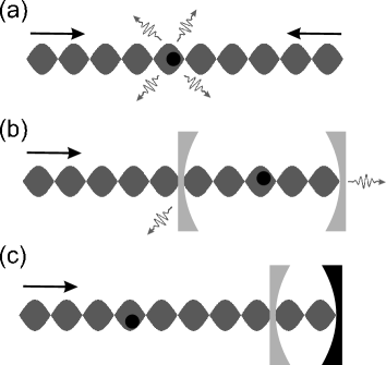
Figure 1: Schematics of optical cooling methods: (a) Free-space laser cooling, (b) cavity-mediated cooling of a particle between two partially reflective mirrors, (c) mirror-mediated cooling of a particle using one perfectly reflecting and one partially reflective mirror.

We start our discussion with a brief review of the fundamental concepts behind three different laser cooling schemes: (i) free-space laser cooling, (ii) cavity-mediated cooling, and (iii) mirror-mediated cooling.

Free-space laser cooling methods, such as Doppler cooling Gordon , polarization gradient cooling polgrad , or velocity-selected coherent population trapping vscpt , utilize a number of laser beams focused from various directions on a small sample of atoms, as illustrated in Fig. 1(a). In each case, the laser and atomic configuration is set up in such a way that the atom-light coupling is velocity-dependent. For example, the photon scattering rate or the spatial positions where scattering predominantly happens can depend on the atomic velocity, leading to an average net cooling effect. The excess momentum of hot atoms is thereby transferred to spontaneously emitted photons. A mathematical description of the cooling mechanism thus contains a number of classical, stationary laser beams, and a quantum description of the atomic degrees of freedom. To remove the excess momentum, the excited states of the atoms are coupled to a heat bath, which is assumed to be memory-less (Markovian) Gardiner .

In cavity-mediated cooling schemes PRL ; Vuletic ; JOSAB ; Maunz , Fig. 1(b), the atoms sit inside an optical resonator and are coupled to one or a few resonator modes, while laser beams are used to pump the resonator through its mirrors. Dipole coupling transfers excess momentum coherently from the atoms to the cavity modes, which subsequently decay through the partially-transmitting mirrors. Mathematically, the classical stationary laser beams are now coupled to a quantum system comprising the atom degrees of freedom and the quantum state of the discrete cavity modes. The modes in turn are coupled to a Markovian heat bath.

In mirror-mediated cooling, finally, the particles sit outside a coherent delay device, Fig. 1(c), which could be as simple as a single mirror, a piece of optical fiber with an inscribed Bragg grating, or formed by an integrated optical resonator on a chip Vahala ; Schmiedmayer ; Reichel ; Mabuchi ; Baumberg . Via the dipole coupling, the particle imprints a phase on the pump beam which returns to the position of the particle after reflection with a time delay. Hence, the total dipole potential experienced by the particle depends on the interference of the incoming beam with the time-delayed reflected beam. If the particle has moved during the light round trip, this leads to a non-conservative force that can be exploited for extracting energy from the particle motion. A mathematical description of this situation therefore requires two key ingredients, different from free-space cooling and cavity-mediated cooling: (i) the pump beam itself must be described as dynamic, and (ii) cooling relies on the system state at an earlier time, thus it is non-Markovian. On the other hand, no heat bath is required.

Instead of introducing a system memory in time, we may also decompose the field into a continuum of modes. The model presented here will follow this latter approach. For the sake of simplicity, we model the polarizable particle as a single two-level atom and assume that the time delay arises from a significant distance (several meters) between the atom and the mirror. However, it is envisaged that in a practical realization the time delay will arise from reflection by an integrated micro-optical resonator or a similar structure. Moreover, we restrict the analysis to a single spatial dimension. The electromagnetic modes at angular frequency $\omega$ thus are standing waves with mode functions $f(\omega,x)=\sin(\omega x/c)$ if the mirror is assumed at $x=0$. Upon adiabatic elimination of the internal degrees of freedom of the atom, and treating atomic motion semiclassically, we obtain a continuum quantum model governed by the Hamiltonian

$$\hat{H} = \int\hbar(\omega-\omega_{0})\hat{a}^{\dagger}(\omega)\hat{a}(\omega)\mathrm{d}\omega$$ (1)

$$+\hbar\frac{g^{2}}{\Delta}\int\!\!\!\int\sin\frac{\omega_{1}x}{c}\sin\frac{\omega_{2}x}{c}\hat{a}^{\dagger}(\omega_{1})\hat{a}(\omega_{2})\mathrm{d}\omega_{1}\mathrm{d}\omega_{2}\quad\quad$$

where $\hat{a}(\omega)$ and $\hat{a}^{\dagger}(\omega)$ are the mode annihilation and creation operators, $\Delta$ is the detuning of the atom from the driving laser, and $g$ is the atom-field coupling constant. For a two-level atom with transition wavelength $\lambda$ and excited state decay rate $2\Gamma$, this coupling constant is related to the mode beam waist $w$ by scat1d

$$2\pi g^{2}=\Gamma\frac{4\sigma_{a}}{\pi w^{2}}$$ (2)

where $\sigma_{a}=3\lambda^{2}/(2\pi)$ is the atomic radiative cross section. The force operator describing the action of the field on an atom at position $x$ is derived from the Hamiltonian as

$$\hat{F}(x)=-\frac{\mathrm{d}\hat{H}}{\mathrm{d}x}.$$ (3)

We note that the general form of the inter-modal coupling given by the Hamiltonian (1) is valid for any point-like dipole scatterer, and thus will also hold for general multi-level atoms and molecules. Moreover, in order to calculate the force (3) we are interested only in the time evolution of the field in the vicinity of the particle. Hence, it is mainly the relative phase between the mode functions at this position which is important. We thus conclude that, instead of free-space propagation, any dispersive optical device could be used as a delay element, which in particular includes resonant micro- or nanostructures.

III Perturbative solution of the model

In the following we apply perturbation theory to the model introduced above to derive the basic properties of the proposed cooling method. We work in the Heisenberg picture where the mode operators become time dependent with the dynamics governed by

$$\frac{\mathrm{d}}{\mathrm{d}t}\hat{a}(\omega,t) = \frac{i}{\hbar}\left[\hat{H},\hat{a}(\omega,t)\right]$$ (4)

$$= -i(\omega-\omega_{0})\hat{a}(\omega,t)$$

$$-\ i\frac{g^{2}}{\Delta}\sin\frac{\omega x}{c}\int\sin\frac{\omega_{1}x}{c}\hat{a}(\omega_{1},t)\mathrm{d}\omega_{1}.$$

Next, we apply a semiclassical approximation for the field modes assuming that the state of every mode is given by a coherent state at all times. This is tantamount to replacing the operator $\hat{a}(\omega,t)$ by its expectation value $a(\omega,t)$. We assume that the atom follows a linear trajectory $x(t)=x+v(t-t_{0})$ such that at a time $t_{0}\gg 2\tau$ the atom is at position $x$. Here, $2\tau=2x/c$ is the round-trip time of the delayed reflection. We then expand the mode amplitudes into powers of both the coupling $g^{2}/\Delta$ and the atom velocity $v$,

$$a(\omega,t)=a_{0}(\omega,t)+\frac{g^{2}}{\Delta}\left[a_{1}(\omega,t)+vb_{1}(\omega,t)\right]+\cdots.$$ (5)

The zeroth order term in $g^{2}/\Delta$ corresponds to the field without back action of the atom. It is thus independent of $v$ and represents the unperturbed driving laser field, which is assumed to be monochromatic,

$$a_{0}(\omega,t)=A\delta(\omega-\omega_{0}).$$ (6)

Here, $|A|^{2}$ gives the pump power in units of photons per second. Inserting (5) with (6) into (4), one can derive the first order terms in $g^{2}/\Delta$ analytically by perturbation theory yielding

$$a_{1}(\omega,t_{0}) = A\frac{\exp\left[-i(\omega-\omega_{0})t_{0}\right]-1}{\omega-\omega_{0}}\sin\frac{\omega x}{c}\sin\frac{\omega_{0}x}{c},$$

$$b_{1}(\omega,t_{0}) = \frac{A}{c}\left[\omega_{0}\sin\frac{\omega x}{c}\cos\frac{\omega_{0}x}{c}+\omega\cos\frac{\omega x}{c}\sin\frac{\omega_{0}x}{c}\right]$$

$$\times\frac{-1+[1+i(\omega-\omega_{0})t_{0}]\exp[-i(\omega-\omega_{0})t_{0}]}{(\omega-\omega_{0})^{2}}.$$

Expressions (5)-(LABEL:eq:b1) can then be inserted into (3) to calculate the leading terms of the force experienced by the atom at position $x$ at time $t_{0}$. Most interesting is the first-order term of the force in velocity $v$, since this gives the linear friction force and thus describes heating or cooling of the atom in the proposed setup. We find

$$F_{v}(x,t_{0})=2\pi\hbar k_{0}^{2}v\tau|A|^{2}\frac{g^{4}}{\Delta^{2}}\sin(4k_{0}x)$$ (9)

in leading order of $x/\lambda$. Here, $k_{0}=\omega_{0}/c$ is the pump wavenumber. Note that $F_{v}$ is independent of time. We now define the spatially dependent friction coefficient $\rho(x)$ by the relation $F_{v}(x)=-\rho(x)mv$ and introduce the atomic saturation parameter $s=|A|^{2}g^{2}/\Delta^{2}$ at the maximum of the standing-wave pump. Together with (2) this yields

$$\rho(x)=-4s\Gamma\frac{\sigma_{\text{a}}}{\pi w^{2}}\frac{\hbar k_{0}^{2}}{m}\tau\sin(4k_{0}x)$$ (10)

which has units of s^-1 and therefore relates to the inverse of the cooling or heating time.

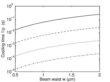
Figure 2: Cooling time of rubidium atoms at position of maximum friction versus beam waist $w$ for $s=0.1$ and $\tau=1$ ns (solid line), 10 ns (dashed), 100 ns (dotted), and 1 $\mu$s (dash-dotted).

Fig. 2 shows the dependence of the 1/e cooling time for rubidium atoms at a point of maximum friction, $\sin(4k_{0}x)=-1$, on the beam waist and for different delay times ranging from 1 ns to 1 $\mu$s. Note that this plot assumes constant saturation $s$ and thus the pump laser power is assumed to increase linearly with the mode area. The figure predicts that cooling times of the order of ms can be achieved if the pump is tightly focussed at the atom and the delay time is of the order of tens of ns. Longer delays lead to faster cooling. These conditions are comparable with those explored experimentally in, for example, Ref. Eschner, .

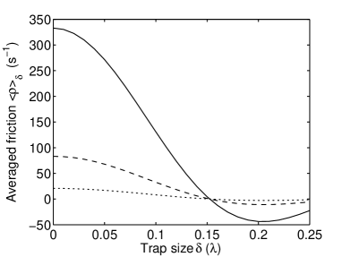
Figure 3: Averaged friction coefficient $\langle\rho(x)\rangle_{\delta}$ for a trap centered at a point of maximum friction versus trap size $\delta$ for $s=0.1$, $\tau=10$ ns, and $w=0.5$ $\mu$m (solid line), $w=1$ $\mu$m (dashes), $w=2$ $\mu$m (dotted).

An important feature of the friction coefficient (10) is its spatial dependence with $\sin(4k_{0}x)$. This implies that the net friction for an extended spatial distribution is zero. Significant cooling via this method thus requires localizing the atom in an additional trap. In practice this could be achieved by an additional far-off resonant beam either propagating parallel to the mirror or forming another standing wave superimposed on the driving beam for the cooling. Alternatively, on-chip microtraps can be utilized in conjunction with integrated time-delay reflectors. In the following, we will assume a harmonic trapping potential. We can then calculate an averaged friction coefficient, defined via the loss of kinetic energy over one oscillation, as

$$\langle\rho(x)\rangle_{\delta} = -4s\Gamma\frac{\sigma_{\text{a}}}{\pi w^{2}}\frac{\hbar k_{0}^{2}}{m}\tau\frac{1}{2\pi}$$ (11)

$$\times\int_{0}^{2\pi}\sin[4k_{0}x+4\delta\sin(T)]\cos^{2}(T)\mathrm{d}T\,\,\,\quad$$

where $\delta$ is the maximum displacement of the atom from the trap center during an oscillation. Fig. 3 shows the averaged friction coefficient versus trap size, assuming that the trap center is at a point of maximum friction. As expected, for increasing $\delta$ the cooling force decreases since the atom moves away from the point of optimum cooling. For trap sizes $\delta\gtrsim 0.15\lambda$ cooling finally turns into heating as the atom spends more time in regions of the standing-wave pump where the mirror-mediated force accelerates the atom.

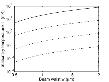
Figure 4: Stationary temperature T at position of maximum friction versus beam waist $w$ for $s=0.1$ and $\tau=1$ ns (solid line), 10 ns (dashed), 100 ns (dotted), and 1 $\mu$s (dash-dotted).

So far, we have neglected momentum diffusion due to spontaneous scattering of photons by the atom, which together with the friction coefficient determines the stationary temperature achievable with this system. To zeroth order in the atom-field coupling, momentum diffusion is due to the interaction with the unperturbed pump field. We may thus expect diffusion to be identical to that observed in free-space Doppler cooling, where the diffusion constant is given by Gordon

$$D=\hbar^{2}k_{0}^{2}\Gamma s.$$ (12)

From this the stationary temperature is obtained as

$$k_{B}T=\frac{D}{m\rho(x)}=\frac{\hbar}{\tau}\frac{\pi w^{2}}{4\sigma_{a}}\frac{-1}{\sin(4k_{0}x)}$$ (13)

where for simplicity we have used the non-averaged value of the friction (10). This is a remarkably simple expression which, apart from the spatial dependence, only depends on the delay time and the beam cross section. Fig. 4 shows the stationary temperatures corresponding to the friction curves of Fig. 2. For realistic parameters these simple analytic results predict stationary temperatures of the order of mK or even slightly below and thus less than an order of magnitude above the Doppler limit of 141 $\mu$K for Rb atoms. However, we emphasize again that the cooling in our scheme is based on the dipole force, in contrast to free-space Doppler cooling which relies on the radiation pressure force. As such, mirror-mediated cooling uniquely also works in the far-off resonant regime.

IV Semiclassical Monte-Carlo simulations

In addition to the perturbative solution of the system dynamics, we also performed numerical Monte-Carlo simulations. These semiclassical simulations have a number of advantages: (i) they allow us to include the harmonic dipole trap consistently, (ii) they provide solutions to any order in the coupling $g^{2}/\Delta$ and in the velocity $v$, and (iii) they include momentum and photon number diffusion. On the other hand, the numerical treatment requires us to restrict the analysis to a discrete set of equally spaced modes of angular frequencies $\omega_{k}$.

The corresponding set of equations is derived following the approach of Refs. sde, which we only very briefly outline here. Starting from the full quantum master equation including quantized atomic motion and a Liouville-type term for spontaneous atomic decay, a Wigner transform is applied to obtain a Fokker-Planck equation for the joint Wigner function of the complex mode field amplitudes $\alpha_{k}$ and the atomic momentum $p$ and position $x$. In the semiclassical approximation, this Fokker-Planck equation is equivalent to the following set of stochastic differential equations:

$$\mathrm{d}x = \frac{p}{m}\mathrm{d}t,$$ (14)

$$\mathrm{d}p = i\gamma\big{[}\mathcal{E}(x)\frac{\mathrm{d}}{\mathrm{d}x}\mathcal{E}^{*}(x)-\mathcal{E}^{*}(x)\frac{\mathrm{d}}{\mathrm{d}x}\mathcal{E}(x)\big{]}\mathrm{d}t$$ (15)

$$-U_{0}\big{[}\mathcal{E}(x)\frac{\mathrm{d}}{\mathrm{d}x}\mathcal{E}^{*}(x)+\mathcal{E}^{*}(x)\frac{\mathrm{d}}{\mathrm{d}x}\mathcal{E}(x)\big{]}\mathrm{d}t$$

$$+k_{t}(x-x_{0})\mathrm{d}t+\mathrm{d}P,$$

$$\mathrm{d}\alpha_{k} = i\Delta_{k}\alpha_{k}\mathrm{d}t-(iU_{0}+\gamma)\mathcal{E}(x)f_{k}^{*}(x)\mathrm{d}t+\mathrm{d}A_{k},\quad$$ (16)

where $\mathcal{E}(x)=\sum_{k}\alpha_{k}\sin(\omega_{k}x/c)$ is the total field amplitude at $x$, $x_{t}$ and $k_{t}$ are the position of the trap center and the trap spring constant, respectively, and $\gamma$ and $U_{0}$ are the atomic scattering rate and the optical potential per photon, respectively. The terms $\mathrm{d}P$ and $\mathrm{d}A_{k}$ are correlated stochastic white-noise terms describing the spontaneous redistribution of photons between modes by the scattering atom and the subsequent fluctuations in atom momentum and modal photon numbers. They are given by sde

$$\mathrm{d}P = k_{0}\sqrt{4\gamma/5}|\mathcal{E}(x)|\mathrm{d}W_{0}+\sqrt{2\gamma}|\frac{\mathrm{d}}{\mathrm{d}x}\mathcal{E}(x)|\mathrm{d}W_{+},$$ (17)

$$\mathrm{d}A_{k} = \sqrt{\gamma/2}\sin\left(\frac{\omega_{k}x}{c}\right)\frac{\frac{\mathrm{d}}{\mathrm{d}x}\mathcal{E}(x)}{|\frac{\mathrm{d}}{\mathrm{d}x}\mathcal{E}(x)|}(i\mathrm{d}W_{+}-\mathrm{d}W_{-}),\quad\quad$$ (18)

where $\mathrm{d}W_{i}$ ($i=0,+,-$) are independent stochastic Ito increments with zero mean, $\langle\mathrm{d}W_{i}\rangle=0$, and unit variance, $\langle\mathrm{d}W_{i}^{2}\rangle=dt$ Gardiner2 .

Unfortunately, discretization of the mode frequencies also implies that the light field is periodic in time with a periodicity given by the inverse spectral mode spacing $2\pi/\Delta\omega$. It is thus not possible to follow a single simulation of the stochastic equations (14)-(16) to a quasi-stationary state. Instead, we perform averages over short propagation times for ensembles of different initial temperatures and derive linear approximations for the rate of temperature change $\mathrm{d}T/\mathrm{d}t$. Numerically, we found that this approach works well, however great care is required in the data analysis and fitting routines as outlined in the following.

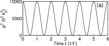
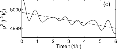
Figure 5: Momentum of a single-particle trajectory in the absence of diffusion. (a) Square of momentum versus time. (b) Detail of (a) with fitted turning points (crosses) using method 1. (c) Fitting method 2: squared momentum after subtraction of a least-square fit with a sine function (solid line) and linear fit to the result (dashed). Parameters are for Rb atoms, $\Delta=-10\Gamma$, $\tau=0.25/\Gamma$, $w=0.7~{}\mu$m, $\Delta\omega=0.1\Gamma$, $\omega_{t}=0.5\times 2\pi\Gamma$, $s=0.076$. The trap is centered at a point of maximum friction.

Figure 5 shows the principles of our data analysis routines for the example of a single particle trajectory, where momentum diffusion was neglected for the sake of clarity. An atom with an initial momentum of 100 $\hbar k_{0}$ oscillates in a trap with trap frequency $\omega_{t}$, Fig. 5(a). A closer look at the maxima of the momentum oscillations, Fig. 5(b), reveals the cooling effect due to friction. Note that this effect is small, only of the order of $10^{-4}$ for the period of time shown here. It is therefore necessary to remove the fundamental oscillation with very high accuracy from the simulated data, as it can otherwise easily mask the effects of friction.

One possibility (method 1) is to fit each single oscillation with a harmonic motion. From these fits the positions and momentum amplitudes of the individual oscillations are obtained, as indicated by the crosses in the figure. Finally, a linear fit to these data points provides an accurate measure of the averaged friction coefficient which can be compared to the analytic result (11). An alternative method (method 2) to extract the friction coefficient from a trajectory, or from an ensemble average over many trajectories in the presence of noise, is shown in Fig. 5(c). In this case, a single sine function is fitted to the trajectory and subtracted from it. The result is a curve where the large amplitude oscillations have been removed. A linear fit to this curve reveals the average slope and thus the friction coefficient. Both methods, 1 and 2, work well within certain parameter limits, with method 1 in general being more accurate but method 2 being quicker to evaluate.

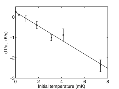
Figure 6: Cooling rate $\mathrm{d}T/\mathrm{d}t$ versus initial temperature. The data points (crosses) and error bars are obtained from Monte-Carlo simulations using $10^{4}$ trajectories per initial temperature. The solid line is a linear fit to the numerical data. The parameters are as in Fig. 5.

The results of one set of simulations of the full system of stochastic differential equations (14)-(16) are shown in Fig. 6. Simulations were performed in ensembles of $10^{4}$ independent trajectories, where the initial conditions of each ensemble were chosen to represent an atomic cloud at a given temperature. Every trajectory was propagated for a time 60 $\Gamma^{-1}$, and ensemble averages of the squared momentum were taken as a measure of the ensemble temperature as a function of time. Finally, method 2 as outlined above was employed to extract a linear approximation to the cooling rate $\mathrm{d}T/\mathrm{d}t$. The numerical errors related to the finite number of simulations per ensemble were estimated by applying the same analysis to sub-ensembles of $10^{3}$ trajectories.

Figure 6 shows that the numerically obtained values of $\mathrm{d}T/\mathrm{d}t$ are well approximated by a linear function of initial temperature. This linear behavior is expected for Brownian motion with linear friction. For very small initial temperatures, momentum diffusion dominates and the ensemble temperature increases with time. For large initial temperatures, on the other hand, friction dominates and the ensemble is cooled. The stationary temperature where the two effects cancel is obtained as $T=0.69\pm 0.17$ mK from the linear fit to the data with Gaussian error propagation. By comparison, the simple analytic estimate (13) predicts a temperature of 0.76 mK, which is in surprisingly good agreement given the number of approximations made in the derivation of the perturbative result.

V Outlook: Application to Micro- and Nanodevices

In the analysis presented above, the delay time was provided by a meter-scale distance between the particle and the mirror. However, we envisage various routes for integration of this cooling scheme into microchip devices, as outlined in the following.

Microresonators. The necessary delay time can be conveniently achieved using an integrated optical resonator Vahala ; Schmiedmayer ; Reichel ; Mabuchi ; Baumberg instead of a delay line. For example, a 10 ns delay requires a resonator quality factor of $Q\approx 10^{7}$, which is well within the limits of state-of-the-art microsphere or microdisk resonators. The friction coefficient $\rho$ will then correspond to the average of Eq. (10) over the delay time $\tau$ for light exiting the resonator after 1, 2, 3, etc. roundtrips.

Plasmonic field enhancement. In free space, the minimum beam diameter is limited by diffraction to about one optical wavelength. However, it has been shown that microantennas can vastly enhance local field intensities by plasmon effects, and enhancement factors of 300 have already been demonstrated Fischer . If the particle could be placed inside such a microantenna, the geometric factor $\sigma_{a}/(\pi w^{2})$ would effectively be increased by this factor, leading to significantly faster, more efficient cooling.

Optomechanics. The scheme discussed in this paper is concerned with cooling of microscopic particles. However, conceptually the proposed cooling method could also be applied to larger objects, e.g., micromechanical mirrors or oscillators Corbitt ; Schliesser ; Xuereb by appropriate device design and scaling of parameters.

With such generalizations we expect that this cooling scheme may be exploited in integrated atom chips atomchip , quantum information processors QIP , atomic clocks clock , or interferometric sensors sensor .

VI Conclusions

We have analyzed theoretically an optical cooling scheme for neutral particles which, in principle, is not restricted to atoms but can be extended to any polarizable species. The scheme exploits the finite delay-time of light propagating from the particle to a mirror and back to the particle, and is thus non-Markovian in nature, in contrast to free-space laser cooling or cavity-mediated cooling methods. Finally, we proposed extensions of the cooling scheme to chip-based devices, which will open the road towards practical applications.

- (1) S. Chu, Rev. Mod. Phys. 70, 685 (1998); C. N. Cohen-Tannoudji, Rev. Mod. Phys. 70, 707 (1998); W. D. Phillips, Rev. Mod. Phys. 70, 721 (1998).
- (2) P. Horak, G. Hechenblaikner, K. M. Gheri, H. Stecher, and H. Ritsch, Phys. Rev. Lett. 79, 4974 (1997).
- (3) V. Vuletic and S. Chu, Phys. Rev. Lett. 84, 3787 (2000).
- (4) P. Domokos and H. Ritsch, J. Opt. Soc. Am. B 20, 1098 (2003).
- (5) P. Maunz, T. Puppe, I. Schuster, N. Syassen, P. W. H. Pinkse, and G. Rempe, Nature 428, 50 (2004).
- (6) A. Xuereb, P. Horak, and T. Freegarde, Phys. Rev. A in press.
- (7) K. J. Vahala, Nature 424, 839 (2003).
- (8) X. Liu, K.-H. Brenner, M. Wilzbach, M. Schwarz, T. Fernholz, and J. Schmiedmayer, Appl. Opt. 44, 6857 (2005).
- (9) T. Steinmetz, Y. Colombe, D. Hunger, T. W. Hänsch, A. Balocchi, R. J. Warburton, and J. Reichel, Appl. Phys. Lett. 89, 111110 (2006).
- (10) P. E. Barclay, K. Srinivasan, O. Painter, B. Lev, and H. Mabuchi, Appl. Phys. Lett. 89, 131108 (2006).
- (11) M. Trupke, F. Ramirez-Martinez, E. A. Curtis, J. P. Ashmore, S. Eriksson, E. A. Hinds, Z. Moktadir, C. Gollasch, M. Kraft, G. V. Prakashb, and J. J. Baumberg, Appl. Phys. Lett. 88, 071116 (2006).
- (12) A. Alù and N. Engheta, Nature Photon. 2, 307 (2008).
- (13) H. Fischer and O. J. F. Martin, Opt. Express 16, 9144 (2008).
- (14) J. P. Gordon and A. Ashkin, Phys. Rev. A 21, 1606 (1980).
- (15) P. Lett, R. Watts, C. Westbrook, W. D. Phillips, P. Gould, and H. Metcalf, Phys. Rev. Lett. 61, 169 (1988).
- (16) A. Aspect, E. Arimondo, R. Kaiser, N. Vansteenkiste, and C. Cohen-Tannoudji, Phys. Rev. Lett. 61, 826 (1988).
- (17) C. W. Gardiner and P. Zoller, Quantum Noise, 3rd ed., Springer, Berlin (2004).
- (18) P. Domokos, P. Horak, and H. Ritsch, Phys. Rev. A 65, 033832 (2002).
- (19) P. Bushev, A. Wilson, J. Eschner, C. Raab, F. Schmidt-Kaler, C. Becher, and R. Blatt, Phys. Rev. Lett. 92, 223602 (2004).
- (20) P. Domokos, P. Horak, and H. Ritsch, J. Phys. B: At. Mol. Opt. Phys. 34, 187 (2001); P. Horak and H. Ritsch, Phys. Rev. A 64, 033422 (2001).
- (21) C. W. Gardiner, Handbook of Stochastic Methods, 3rd ed., Springer, Berlin (2004).
- (22) T. Corbitt, C. Wipf, T. Bodiya, D. Ottaway, D. Sigg, N. Smith, S. Whitcomb, and N. Mavalvala, Phys. Rev. Lett. 99, 160801 (2007).
- (23) A. Schliesser, R. Rivière, G. Anetsberger, O. Arcizet, and T. J. Kippenberg, Nature Phys. 4, 415 (2008).
- (24) A. Xuereb, P. Domokos, J. Asbóth, P. Horak, and T. Freegarde, Phys. Rev. A 79, 053810 (2009).
- (25) R. Folman, P. Krüger, J. Schmiedmayer, J. Denschlag, and C. Henkel, Adv. At. Mol. Opt. Phys. 48, 263 (2002).
- (26) M. A. Nielsen and I. L. Chuang, Quantum Computation and Quantum Information, Cambridge University Press, Cambridge (2000).
- (27) G. Santarelli, P. Laurent, P. Lemonde, A. Clairon, A. G. Mann, S. Chang, A. N. Luiten, and C. Salomon, Phys. Rev. Lett. 82, 4619 (1999).
- (28) W. Hänsel, J. Reichel, P. Hommelhoff, and T. W. Hänsch, Phys. Rev. A 64, 063607 (2001).