Scale Dependence of Halo Bispectrum from Non-Gaussian Initial Conditions in Cosmological N-body Simulations

Abstract

We study the halo bispectrum from non-Gaussian initial conditions. Based on a set of large $N$-body simulations starting from initial density fields with local type non-Gaussianity, we find that the halo bispectrum exhibits a strong dependence on the shape and scale of Fourier space triangles near squeezed configurations at large scales. The amplitude of the halo bispectrum roughly scales as $f_{\rm NL}^{2}$. The resultant scaling on the triangular shape is consistent with that predicted by Jeong & Komatsu based on perturbation theory. We systematically investigate this dependence with varying redshifts and halo mass thresholds. It is shown that the $f_{\rm NL}$ dependence of the halo bispectrum is stronger for more massive haloes at higher redshifts. This feature can be a useful discriminator of inflation scenarios in future deep and wide galaxy redshift surveys.

1 Introduction

The standard cosmological model has successfully explained the observed statistical properties of the cosmic microwave background (CMB) radiation and the large scale structure (LSS) traced by galaxies (e.g., [1, 2]). The model usually assumes that the primordial density/temperature/curvature fluctuations follow Gaussian statistics. Recently, however, possible deviations from standard Gaussian statistics has attracted great attention with rapid progress in observational techniques. It offers an opportunity to access cosmological information beyond traditional power spectrum analysis. Many recent works have discussed the constraints and future detectability of possible deviations from Gaussianity through the observations of CMB and LSS (e.g., [3, 4]).

According to the inflationary scenarios, primordial curvature perturbations are generated during the accelerated phase of cosmic expansion. The simplest inflation models, in which the inflation takes place with the slow-roll single scalar field that has a canonical kinetic structure, generally predicts a nearly scale-invariant spectrum of curvature perturbations, and a small departure from Gaussianity. On the other hand, a variety of inflation models that produce a large non-Gaussianity has been recently proposed (see [5] for a review). Among these, the models with large non-Gaussianity generated by non-linear dynamics on super-horizon scales can have a generic prediction for non-Gaussian properties. Denoting a Gaussian field by $\Phi_{\rm G}(\mbox{\boldmath$x$})$, the Bardeen’s curvature perturbation during the matter era is characterized as [3]:

$$\Phi(\mbox{\boldmath$x$})=\Phi_{\rm G}(\mbox{\boldmath$x$})+f_{\rm NL}\left\{\Phi_{\rm G}^{2}(\mbox{\boldmath$x$})-\langle\Phi_{\rm G}^{2}(\mbox{\boldmath$x$})\rangle\right\}+\cdots.$$ (1)

This type of non-Gaussianity, described as a local function of the Gaussian field, is often called local type non-Gaussianity, and the leading-order coefficient $f_{\rm NL}$, which controls the strength of non-Gaussianity, has information on the generation mechanisms for non-Gaussian fluctuations. Although the current constraint on the parameter $f_{\rm NL}$ from CMB data is $-9<f_{\rm NL}<111$ ($95\%$C.L.) [1] and it is still consistent with Gaussian ($f_{\rm NL}=0$), the constraint will be tightened by the on-going CMB experiment, Planck [6]. As standard inflation models generally predict $|f_{\rm NL}|\ll 1$, detection of large non-Gaussianity immediately implies the non-standard mechanism for generation of primordial curvature perturbations.

In this paper, we focus on how this type of non-Gaussianity alters the statistical properties of LSS. Let us first define the power spectrum of mass density fluctuations assuming isotropy and homogeneity:

$$\langle\delta_{\rm m}(\mbox{\boldmath$k$}_{1})\delta_{\rm m}(\mbox{\boldmath$k$}_{2})\rangle\equiv(2\pi)^{3}\delta_{\rm D}(\mbox{\boldmath$k$}_{1}+\mbox{\boldmath$k$}_{2})P_{\rm m}(k_{1}),$$ (2)

where $\delta_{\rm m}(\mbox{\boldmath$k$})$ denotes the Fourier transform of the density contrast, while $\delta_{\rm D}(\mbox{\boldmath$k$})$ represents the Dirac delta function. If the density field follows Gaussian statistics, its power spectrum determines all the statistical properties. Next we define the bispectrum of a mass density field:

$$\langle\delta_{\rm m}(\mbox{\boldmath$k$}_{1})\delta_{\rm m}(\mbox{\boldmath$k$}_{2})\delta_{\rm m}(\mbox{\boldmath$k$}_{3})\rangle\equiv(2\pi)^{3}\delta_{\rm D}(\mbox{\boldmath$k$}_{1}+\mbox{\boldmath$k$}_{2}+\mbox{\boldmath$k$}_{3})B_{\rm m}(\mbox{\boldmath$k$}_{1},\mbox{\boldmath$k$}_{2},\mbox{\boldmath$k$}_{3}).$$ (3)

Since this is the lowest-order non-vanishing quantity in the presence of non-Gaussianity, the bispectrum is naively expected as the best measure for non-Gaussianity (e.g., [7, 8, 9, 10]).

Recently, however, the galaxy or halo power spectrum has been reconsidered in the presence of local and/or equilateral type primordial non-Gaussianity both analytically and numerically (e.g., [11, 12, 13, 14, 15, 16, 17, 18, 19, 20, 21, 22]). The matter power spectrum or bispectrum is not a direct observable, and the real measurement of LSS gives galaxy power spectrum or bispectrum, as defined similarly to equations (2) and (3). Since galaxies are biased tracers of the dark matter distribution, the information of $f_{\rm NL}$ is imprinted in a different manner: a new contribution coming from the primordial non-Gaussianity may dominate over the Gaussian term in the galaxy power spectrum, $P_{\rm g}(k)$, at very large scales ($k\lower 2.15277pt\hbox{$\;\buildrel<\over{\sim}\;$}0.01h$Mpc^-1). This new contribution, which is sometimes referred to as the “scale-dependent bias” of the galaxy power spectrum, may be a powerful indicator to constrain $f_{\rm NL}$. Indeed, it has been recently applied to the clustering statistics of SDSS LRG and quasar samples, and the tight constraints on $f_{\rm NL}$ are comparable to those obtained from CMB measurements have been obtained [19].

The purpose of this paper is to examine the bispectrum of biased tracers in detail. While the matter bispectrum in the presence of primordial non-Gaussianity has been studied in the literature using both perturbation theory and numerical simulations, the galaxy bispectrum may significantly differ from the matter bispectrum in the presence of primordial non-Gaussianity, just like the difference in the power spectra. Since the local type non-Gaussianity can be straightforwardly implemented within $N$-body simulations, numerical study on the bispectrum for the dark matter haloes is the first important step toward a practical understanding of the galaxy bispectrum.

Incidentally, Jeong and Komatsu (2009) recently proposed a new parametrized model for the halo/galaxy bispectrum ([23], see also [21]) based on the peak bias model [24] and the local bias model [25]. They found that the formula for the galaxy bispectrum used in [10] was missing important contributions from the scale dependent bias effects and they discovered new terms that are important at “squeezed” configurations where $k_{1},k_{2}\gg k_{3}$. It was argued that these new contributions enable us to put stronger constraints on $f_{\rm NL}$ than those obtained in [10]. It is of great importance to confirm the scale-dependent bias effects in the bispectrum by $N$-body simulations.

The rest of this paper is organized as follows: we first review the analytical models of the power spectrum and the bispectrum of biased tracers in section 2. We then describe the setup and initial conditions for $N$-body simulations in section 3. As a first check of our simulations, in section 4, we compute the matter and halo power spectra, and the results are compared with previous works. Section 5 gives the main results of this paper, in which the simulation results for the matter and halo bispectra are presented and compared with predictions from analytic models, particularly focusing on their scale dependence. The dependence of the halo bispectrum on the halo mass threshold and redshift is also investigated in detail. Section 6 discusses the future prospects for detecting the primordial non-Gaussianity using the scale-dependent properties of the halo/galaxy bispectrum. Finally, section 7 is devoted to conclusions and discussions.

2 Theoretical models

In this section, we summarize the theoretical predictions of the power spectrum and bispectrum. We use perturbation theory to examine the matter power spectrum and bispectrum, and then present those of biased tracers based on the local bias model. For the scales of our interest ($k\lower 2.15277pt\hbox{$\;\buildrel<\over{\sim}\;$}0.1h$ Mpc^-1), the non-linearity of gravitational evolution is moderate and the perturbation theory is valid and trustful. We especially focus on the behavior of the bispectrum in the squeezed limit on large scales, where $k\equiv k_{1}=k_{2}\equiv\alpha k_{3}$, $k\to 0$ and $\alpha\gg 1$.

Let us first consider the matter density fluctuation. We perturbatively expand this as

$$\delta_{\rm m}(\mbox{\boldmath$k$};z)=\delta_{\rm m}^{(1)}(\mbox{\boldmath$k$};z)+\delta_{\rm m}^{(2)}(\mbox{\boldmath$k$};z)+\delta_{\rm m}^{(3)}(\mbox{\boldmath$k$};z)+\cdots.$$ (4)

The linear-order solution is related to the Bardeen’s curvature perturbation in equation (1) in Fourier space by

$$\delta_{\rm m}^{(1)}(\mbox{\boldmath$k$};z)={\cal M}(k;z)\Phi(\mbox{\boldmath$k$}),$$ (5)

where the conversion factor $\mathcal{M}$ is defined as

$${\cal M}(k;z)\equiv\frac{2}{3}\frac{k^{2}T(k)D(z)}{\Omega_{\rm m}H_{0}^{2}}.$$ (6)

In the above, $\Omega_{\rm m}$ is the current matter density normalized by the critical density, $H_{0}$ is current Hubble constant, $T(k)$ denotes the matter transfer function normalized to unity at $k\to 0$ and $D(z)$ is the linear growth rate normalized to the scale factor in the limit of matter dominant era. The higher-order solutions, $\delta_{\rm m}^{(n)}(\mbox{\boldmath$k$};z)$, are formally written as

$$\delta_{\rm m}^{(n)}(\mbox{\boldmath$k$};z)=\int d^{3}\mbox{\boldmath$q$}_{1}\cdots d^{3}\mbox{\boldmath$q$}_{n}\delta_{\rm D}(\mbox{\boldmath$k$}-\mbox{\boldmath$q$}_{1\dots n})F_{n}(\mbox{\boldmath$q$}_{1},\dots,\mbox{\boldmath$q$}_{n})\delta_{\rm m}^{(1)}(\mbox{\boldmath$q$}_{1};z)\cdots\delta_{\rm m}^{(1)}(\mbox{\boldmath$q$}_{n};z),$$ (7)

where $\mbox{\boldmath$q$}_{1\dots n}\equiv\mbox{\boldmath$q$}_{1}+\cdots+\mbox{\boldmath$q$}_{n}$, and $F_{n}$ are the kernel functions (see [26] for a review). Then keeping terms up to fourth order in $\delta_{\rm m}^{(1)}$, the power spectrum and bispectrum of the matter density fluctuations are given by (e.g., [13, 10])

$$P_{\rm m}(k;z) = P_{0}(k;z)\;+\;2\int\frac{d^{3}\mbox{\boldmath$q$}}{(2\pi)^{3}}F_{2}(\mbox{\boldmath$q$},\mbox{\boldmath$k$}-\mbox{\boldmath$q$})B_{0}(-\mbox{\boldmath$k$},\mbox{\boldmath$q$},\mbox{\boldmath$k$}-\mbox{\boldmath$q$};z)$$ (8)

$$+\;2\int\frac{d^{3}\mbox{\boldmath$q$}}{(2\pi)^{3}}\left\{F_{2}(\mbox{\boldmath$q$},\mbox{\boldmath$k$}-\mbox{\boldmath$q$})\right\}^{2}P_{0}(q;z)P_{0}(|\mbox{\boldmath$k$}-\mbox{\boldmath$q$}|;z)$$

$$+\;\int\frac{d^{3}\mbox{\boldmath$p$}d^{3}\mbox{\boldmath$q$}}{(2\pi)^{6}}F_{2}(\mbox{\boldmath$p$},\mbox{\boldmath$k$}-\mbox{\boldmath$p$})F_{2}(\mbox{\boldmath$q$},-\mbox{\boldmath$k$}-\mbox{\boldmath$q$})T_{0}(\mbox{\boldmath$p$},\mbox{\boldmath$k$}-\mbox{\boldmath$p$},\mbox{\boldmath$q$},-\mbox{\boldmath$k$}-\mbox{\boldmath$q$};z),$$

$$+P_{0}(k;z)\int\frac{\rmd^{3}\mbox{\boldmath$q$}}{(2\pi)^{3}}F_{3}(\mbox{\boldmath$k$},\mbox{\boldmath$q$},-\mbox{\boldmath$q$})P_{0}(q;z),$$

$$B_{\rm m}(k_{1},k_{2},k_{3};z) = 2f_{\rm NL}\left[\frac{P_{0}(k_{1};z)P_{0}(k_{2};z)\mathcal{M}(k_{3};z)}{\mathcal{M}(k_{1};z)\mathcal{M}(k_{2};z)}+({\rm cyc.})\right]$$ (9)

$$+2F_{2}(\mbox{\boldmath$k$}_{1},\mbox{\boldmath$k$}_{2})P_{0}(k_{1};z)P_{0}(k_{2};z)+({\rm cyc.}),$$

where $({\rm cyc.})$ denotes the cyclic permutations over the indices and $P_{0}$, $B_{0}$, and $T_{0}$ are the power-, bi-, and tri-spectra of $\delta_{\rm m}^{(1)}$. In equation (8), the second term is the first non-trivial correction in the presence of primordial non-Gaussianity, and the function $B_{0}$ implies the primordial bispectrum, which corresponds to the leading-order contribution in equation (9). Note that the contribution coming from the primordial trispectrum $T_{0}$ is small for local type non-Gaussianity with reasonable values of $f_{\rm NL}$, and we drop this term in computing $P_{\rm m}$ (see [13]).

On the other hand, the power spectrum of biased tracers has been recently discussed in the literature [11, 14, 19, 12, 20, 13], based on several different formalisms including peak bias, halo bias according to the peak-background split, and local bias. The resultant expressions of the galaxy/halo power spectrum are basically the same, and are summarized in the form

$$P_{\rm g}(k;z) = b_{1}^{2}\left\{1\;+\;2\;\frac{\tilde{b}_{2}}{b_{1}}\;f_{\rm NL}\;\mathcal{M}^{-1}(k;z)\right\}^{2}\;P_{0}(k;z),$$ (10)

where $b_{1}$ and $\tilde{b}_{2}$ are the bias parameters relating the galaxy overdensity to the matter overdensity. In A, we present a derivation of (10) based on the local bias formalism. The explicit expressions for the bias parameters $b_{1}$ and $\tilde{b}_{2}$ can be obtained both from the peak bias and halo bias formalisms, and their results are basically the same in the high-peak/threshold limit. In B, we show that in the high-peak limit, there is a clear relationship between the peak bias and the local bias prescriptions, and the parameters $b_{1}$ and $\tilde{b}_{2}$ are related to each other in terms of the critical density of the spherical collapse model, $\delta_{\rm c}\approx 1.686$, as $\tilde{b}_{2}=\delta_{\rm c}\;(b_{1}-1)$.

In equation (10), the factor in the braces manifestly depends on the scale, which is the main source for “scale-dependent bias”. On large scales ($k\to 0$), the function $\mathcal{M}$ is roughly proportional to $k^{2}$, and it strongly affects the galaxy power spectrum. In this respect, the scale-dependent property will be a clear indicator of primordial non-Gaussianity of the local type, and it has been extensively tested against $N$-body simulations. Several recent studies have suggested that some modifications to this formula are required in order to model the scale-dependent bias more accurately [15, 16, 18]. For example, [18] proposed a slight modification to the relation of bias parameters, which reproduces results from $N$-body simulations very well:

$$\tilde{b}_{2}=\delta_{\rm c}\;q\;(b_{1}-1),$$ (11)

with $q=0.75$, which comes from the ellipsoidal collapse model.

Now, we turn our focus to the bispectrum of biased tracers in the presence of primordial non-Gaussianity. According to the analytical study by [23] (see also [21]), the effect of local-type primordial non-Gaussianity is mainly imprinted on the bispectrum of squeezed triangular configurations. The galaxy bispectrum is then expressed as

$$B_{\rm g}(k,\alpha;z) = B_{\rm g}^{(0)}(k,\alpha;z)+f_{\rm NL}\,B_{\rm g}^{(1)}(k,\alpha;z)+f_{\rm NL}^{2}\,B_{\rm g}^{(2)}(k,\alpha;z),$$ (12)

where each term of the right-hand side of this equation has the following asymptotic form:

$$B_{\rm g}^{(0)}(k,\alpha;z) \simeq b_{1}^{2}\,b_{2}\,P_{k\to 0}^{2}(z)\,k^{2n_{s}}\,\alpha^{0},$$ (13)

$$B_{\rm g}^{(1)}(k,\alpha;z) \simeq \left[4b_{1}^{3}+\left(\frac{26}{7}+{\cal I}(k,\alpha;R)\right)b_{1}^{2}\tilde{b}_{2}\right]\,P_{k\to 0}^{2}(z)\,{\cal M}_{k\to 0}^{-1}(z)\,k^{2n_{s}-2}\,\alpha^{1},$$

$$B_{\rm g}^{(2)}(k,\alpha;z) \simeq 8\,b_{1}^{2}\,\tilde{b}_{2}\,P_{k\to 0}^{2}(z)\,{\cal M}_{k\to 0}^{-2}(z)\,k^{2n_{s}-4}\,\alpha^{3}.$$ (15)

Here, we focused on the isosceles triangles, and parametrized their dependence as $k\equiv k_{1}=k_{2}\equiv\alpha k_{3}$, and $n_{\rm s}$ denotes the scalar spectral index. See A for a more rigorous expression. The function ${\cal I}(k,\alpha;R)$ weakly depends on $k,\alpha$ and the smoothing scale, $R$, and it can be approximated as $26/7+{\cal I}(k,\alpha;R)\sim 34$ on large scales. In the above, we take the limit of $k\to 0$ and $\alpha\gg 1$, and $P_{k\to 0}$, $\mathcal{M}_{k\to 0}$ are defined through $P_{0}(k;z)\to P_{k\to 0}(k)k^{n_{\rm s}}$, $\mathcal{M}(k;z)\to\mathcal{M}_{k\to 0}(z)k^{2}$. See A and also [23] for more details.

Similar to the scale dependence of the galaxy/halo power spectrum in equation (10), the amplitude of bispectrum is also affected by the primordial non-Gaussianity in a scale-dependent way. In particular, the term $B_{\rm g}^{(2)}$, which is of quadratic order in $f_{\rm NL}$, becomes dominant on large scales and exhibits a behavior strongly dependent on $k$ and $\alpha$. Thus, we might conclude that this is the most important indicator of $f_{\rm NL}$, capable of detecting the primordial non-Gaussianity with upcoming galaxy surveys of large volumes.

In what follows, we will examine this scale dependence in the bispectrum of simulated dark matter haloes, with particular attention on the squeezed configurations on large scales.

3 $N$-body Simulations

3.1 Setup

We adopt the WMAP5 best-fit flat $\Lambda$CDM model [1]: $\Omega_{\rm m}=0.279$, $\Omega_{\Lambda}=0.721$, $\Omega_{\rm b}=0.046$, $h=0.701$, $\sigma_{8}=0.817$ and $n_{s}=0.96$, where $\Omega_{\rm m}$, $\Omega_{\Lambda}$ and $\Omega_{\rm b}$ are the matter density, cosmological constant and the baryon density normalized by the critical density, $h$ is Hubble constant normalized by $100\,$km s^-1Mpc^-1, $\sigma_{8}$ is the r.m.s. linear density fluctuation smoothed by a top hat window function with radius of $8h^{-1}$Mpc and $n_{\rm s}$ is the scalar spectral index. We calculate the linear matter transfer function using the CAMB code [27]. We have completed a total of $140$ realizations of matter clustering data: $20$ per each of the seven values for the local-type primordial non-Gaussianity parameter, $f_{\rm NL}=0$, $\pm 100$, $\pm 300$ and $\pm 1000$. All the simulations were ran with the Gadget2 code [28]. We adopt $N=512^{3}$ particles in boxes of side $2000h^{-1}$Mpc, and set the softening length being $0.2h^{-1}$Mpc. The parameters adopted in the simulations are the same as in [29, 30]. We have tested the mass/force resolution by changing the box size and found that the results are well converged at large scales ($\sim 1\%$ accuracy at $k\lower 2.15277pt\hbox{$\;\buildrel<\over{\sim}\;$}0.3h$Mpc^-1) for the matter power spectrum.

In setting the initial conditions, we first generate a random Gaussian field, $\Phi_{\rm G}$, whose power spectrum is proportional to $k^{n_{\rm s}-4}$. We then apply the inverse Fourier transform, and add the non-Gaussian contributions in real space according to equation (1). Finally the real-space quantity is transformed back to the Fourier space, and converted to the linear density fluctuations by multiplying $\mathcal{M}(k;z)$ defined in equation (6). We use second-order Lagrangian perturbation theory to calculate the displacement field for $512^{3}$ particles placed on a regular lattice [31] at $z=31$.

We store outputs at $z=2$, $1$ and $0.5$, and identify haloes for each output using a FOF group finder with linking length of $0.2$ times the mean separation. We select haloes in which the number of particles, $N$, is equal to or larger than $10$, corresponding to the haloes with masses $4.6\times 10^{13}h^{-1}M_{\odot}$. We also analyze haloes with $N\geq 20$ and $N\geq 30$ to see the dependence on halo mass.

As a first check of the reliability of our simulations, we show in Fig. 1 the ratio of halo mass function with and without primordial non-Gaussianity, $R(M;f_{\rm NL})\equiv n_{\rm nG}(M;f_{\rm NL})/n_{\rm G}(M)$, at $z=0.5$, where different colors correspond to different values of $f_{\rm NL}$: $1000$, $300$, $100$, $0$, $-100$, $-300$ and $-1000$ from top to bottom. Both simulations and theoretical models suggest that the local type non-Gaussianity alters the mass function at the high-mass tail in the literature: a positive (negative) $f_{\rm NL}$ enhances (suppresses) the tail. As shown in Fig. 1, our simulations agree well with previously proposed analytical models. The plotted lines show the model proposed by [32] (solid):

$$R(M;f_{\rm NL})=1+\frac{1}{6}\frac{\sigma_{\rm R}^{2}}{\delta_{\rm ec}}\left[S_{3}\left(\frac{\delta_{\rm ec}^{4}}{\sigma_{\rm R}^{4}}-2\frac{\delta_{\rm ec}^{2}}{\sigma_{\rm R}^{2}}-1\right)+\frac{\rmd(\sigma_{\rm R}S_{3})}{\rmd\ln\sigma_{\rm R}}\left(\frac{\delta_{\rm ec}^{2}}{\sigma_{\rm R}^{2}}-1\right)\right],$$ (16)

based on the Edgeworth expansion to the probability density function, and by [33] (dashed):

$$R(M;f_{\rm NL})=\exp\left(\frac{\delta_{\rm ec}^{3}}{6}\frac{S_{3}}{\sigma_{\rm R}^{2}}\right)\left|\frac{1}{6}\frac{\delta_{\rm ec}}{\sqrt{1-\delta_{\rm ec}S_{3}/3}}\frac{\rmd S_{3}}{\rmd\ln\sigma_{\rm R}}+\sqrt{1-\delta_{\rm ec}S_{3}/3}\right|,$$ (17)

obtained by the saddle-point approximation to the level excursion probability. In the above, $\sigma_{\rm R}\equiv\langle\delta_{\rm m}^{2}\rangle^{1/2}$ and $S_{3}\equiv\langle\delta_{\rm m}^{3}\rangle/\sigma_{\rm R}^{4}$. These quantities are given as the function of mass $M$ through the relation $M=(4\pi/3)\overline{\rho}_{\rm m}\,R^{3}$, and linearly extrapolated to $z=0.5$. We also define $\delta_{\rm ec}\equiv q\delta_{\rm c}$ again motivated by ellipsoidal collapse model [18]. See also [16] for another model designed to fit to their $N$-body simulations.

There are several claims on the systematics for the estimated halo mass by FOF, and in fact our mass function fits better with [33] when we correct that effect using the empirical formula of [34]. We conclude here that our halo catalog is accurate enough to investigate its clustering statistics.

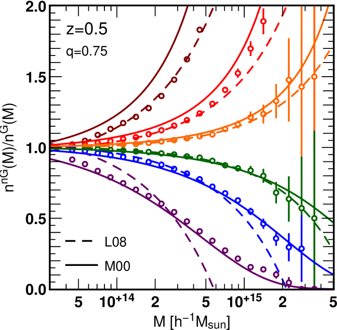
Figure 1: The ratio of the halo mass functions for non-Gaussian and Gaussian initial conditions at $z=0.5$. The symbols show the measurements from our simulations, while the lines are equations (16) and (17). The values of $f_{\rm NL}$ are $1000$, $300$, $100$, $0$, $-100$, $-300$, and $-1000$ from top to bottom.

3.2 Measurements of the power spectrum and bispectrum

Here, we briefly mention how to measure the power spectrum and bispectrum in our simulations.

We assign particles (or haloes) to $1024^{3}$ grid points using the Cloud-in-Cells (CIC) algorithm [35]. We then Fourier transform the density field, and divide each mode by the Fourier transform of the CIC kernel to correct for the effect of assignment. We made sure that the results are well converged at the scale of our interest by changing the number of grid points. We logarithmically divide the measured power spectrum and bispectrum into wave number bins starting from $k_{\rm min}=0.003h$Mpc^-1 and with $10$ bins per decade. We select “isosceles” triangles, whose two longer sides, $k_{1}$ and $k_{2}$, fall into the same bin for the bispectrum analysis. In this sense our isosceles triangles are not strictly isosceles, but we adopt this convention to reduce the statistical errors on the measured bispectrum caused by small number of triangles in $k$-space. In plotting results, we assign each data point to the logarithmic-central value of wave number in that bin.

4 Results of Power Spectrum

In this section, we present the power spectrum measured from $N$-body simulations We first compare the measured matter power spectrum with the perturbation theory prediction. We then present the halo power spectrum, and compare it with the analytic models proposed in the literature. These are important sanity checks to justify the results of our simulations in subsequent sections.

4.1 matter power spectrum

We first examine the matter power spectrum, in cases with non-zero $f_{\rm NL}$. Fig. 2 shows the fractional difference of the matter power spectra between Gaussian and non-Gaussian initial conditions measured at $z=0.5$. The symbols represent $f_{\rm NL}=300,100,0,-100$ and $-300$ from top to bottom at $k\lower 2.15277pt\hbox{$\;\buildrel>\over{\sim}\;$}0.02h$Mpc^-1. Since we use the same set of random seeds for the seven $f_{\rm NL}$ parameters, the cosmic variance is effectively canceled out by taking the ratios, $P_{\rm m}^{\rm nG}(k;z)/P_{\rm m}^{\rm G}(k;z)$. Overall, the deviations from Gaussian results themselves are very small (less than $1\%$ when $|f_{\rm NL}|=100$ in the plotted range).

In Fig. 2, we also plot the predictions based on perturbation theory of [13], depicted as continuous lines. Note that recently, Ref. [36] developed another analytical model based on the Time-RG approach, which would be more accurate in the weakly nonlinear regime. However, the standard perturbation theory prediction of [13] is accurate enough at the scale of our interest (i.e., $k\lower 2.15277pt\hbox{$\;\buildrel<\over{\sim}\;$}0.05h$Mpc^-1), as was shown by comparisons with $N$-body simulations in Refs. [15, 16].

Fig. 2 shows that the results of our $N$-body simulations are in reasonably good agreement with the model of [13], except for the case of a large non-Gaussianity with $f_{\rm NL}=300$. The discrepancy between $N$-body and analytic results seen in the $f_{\rm NL}=300$ case might be partially ascribed to the term coming from the primordial trispectrum in equation (8), which is neglected in the perturbation theory calculations. Nevertheless, the discrepancy remains at the sub-percent level, and thus does not seriously affect the later analysis of the matter/halo bispectrum.

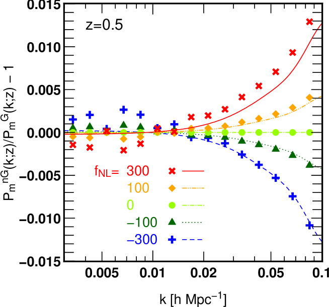
Figure 2: Fractional differences of the matter power spectra starting from non-Gaussian and Gaussian initial conditions. Symbols show the results of $N$-body simulations, while lines are perturbation theory predictions of equation (8) ($f_{\rm NL}=300,100,0,-100,-300$ from top to bottom at $k\lower 2.15277pt\hbox{$\;\buildrel>\over{\sim}\;$}0.02h$Mpc^-1).

4.2 halo power spectrum

We next consider the halo power spectrum for various values of $f_{\rm NL}$, shown in Fig. 3. We set the minimum mass of haloes to $4.6\times 10^{13}h^{-1}M_{\odot}$, which corresponds to $10$ $N$-body particles. We also show the analytical prediction of equation (10) with the bias parameter $b_{1}$ fitted to reproduce the results of Gaussian simulations, adopting the relation between bias parameters in equation (11). We plot the model with $q=1$ and $q=0.75$ by dotted and solid lines, which corresponds to the original peak bias prediction and the fit by [18], respectively.

Overall, the scale dependence of the halo power spectrum discussed in the literature can be clearly seen in our simulations with very small statistical errors, owing to the large total volumes. The agreement between $N$-body simulations and the analytic models becomes better when we choose $q=0.75$, consistent with [18].

Note, however, that the choice of $q=0.75$ does not necessarily imply the best-fit results: $q=0.85$ gives a better fit to this particular case, and the best-fit value of $q$ changes with redshift and minimum halo mass. This might indicate that there exists some systematic effects on the halo clustering properties in our simulations. One possibility is the difference in the halo finding algorithms: while we adopt the FOF finder, [18] use a SO finder. See also [15], where they use a FOF finder and proposed a fit corresponding to $q=0.8$.

We may further improve the agreement between $N$-body simulations and theoretical predictions by including some corrections to the theory. Ref. [16] showed that the inclusion of two corrections coming from the changes in halo mass function and the matter power spectrum actually improves their results. These systematics will definitely be important for the application to the upcoming surveys, however, we do not pursue this issue in the present paper, since our primary focus is on the halo bispectrum.

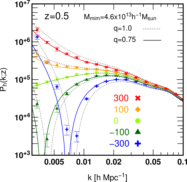
Figure 3: The power spectrum of haloes more massive than $4.6\times 10^{13}h^{-1}M_{\odot}$ at $z=0.5$. Symbols are results of $N$-body simulations, while lines are theoretical prediction of equation (10) with (11) where we adopt $q=1.0$ for dotted lines and $q=0.75$ for solid lines ($f_{\rm NL}=300,100,0,-100,-300$ from top to bottom).

5 Results of Bispectrum

In this section, we present the bispectrum measured from $N$-body simulations. Throughout the analysis, we consider the isosceles triangles for the configuration of bispectrum, which are characterized by the two parameters $k$ and $\alpha$, defined by $k\equiv k_{1}=k_{2}\equiv\alpha k_{3}$. We pay special attention to the squeezed triangles, $\alpha\gg 1$. We first present the results of the matter bispectrum (Sec. 5.1), and then discuss how the halo bispectrum differs from the matter bispectrum (Sec. 5.2). While we mainly analyze the default halo catalog with minimum mass $M_{\rm min}=4.6\times 10^{13}h^{-1}M_{\odot}$ and output redshift $z=0.5$, we briefly discuss how the results are changed when we vary the minimum halo mass and redshift (Sec. 5.2.3).

5.1 matter bispectrum

Let us present the results of the measured matter bispectrum. In Fig. 4, the symbols in each panel show the amplitude of the bispectrum measured from simulations for various $f_{\rm NL}$ at a fixed triangle specified by $k$ and $\alpha$ indicated in the panel. We also show the perturbation theory prediction of equation (9) by solid lines. Note that the value of $\alpha$ increases from right to left, while $k$ increases from top to bottom.

Although we have very large total volume, the statistical uncertainty due to finiteness of the simulated volume still affects the measurements. We thus take account of this effect in the perturbation theory predictions: we compute the matter bispectrum using the second-order perturbation theory starting from linear density field realized in finite-volume boxes which were used to generate the initial conditions of the simulations, and take average over realizations. Namely, we compute

$${\rm Re}\Bigl{[}\delta_{\rm m}^{(1)}(\mbox{\boldmath$k$}_{1})\delta_{\rm m}^{(1)}(\mbox{\boldmath$k$}_{2})\delta_{\rm m}^{(1)}(\mbox{\boldmath$k$}_{3})$$

$$+\delta_{\rm m}^{(2)}(\mbox{\boldmath$k$}_{1})\delta_{\rm m}^{(1)}(\mbox{\boldmath$k$}_{2})\delta_{\rm m}^{(1)}(\mbox{\boldmath$k$}_{3})+\delta_{\rm m}^{(1)}(\mbox{\boldmath$k$}_{1})\delta_{\rm m}^{(2)}(\mbox{\boldmath$k$}_{2})\delta_{\rm m}^{(1)}(\mbox{\boldmath$k$}_{3})+\delta_{\rm m}^{(1)}(\mbox{\boldmath$k$}_{1})\delta_{\rm m}^{(1)}(\mbox{\boldmath$k$}_{2})\delta_{\rm m}^{(2)}(\mbox{\boldmath$k$}_{3})\Bigr{]},$$ (18)

and take the average over the realizations and triangles in the bin for the perturbation theory prediction. As a result, the analytical predictions are in good agreements with measurements from simulations.

The matter bispectrum from both simulations and perturbation theory clearly exhibits a linear dependence on $f_{\rm NL}$ for all the configurations plotted in Fig. 4. Based on this results, we will discuss how the dependence on $f_{\rm NL}$ is modified for the halo bispectrum.

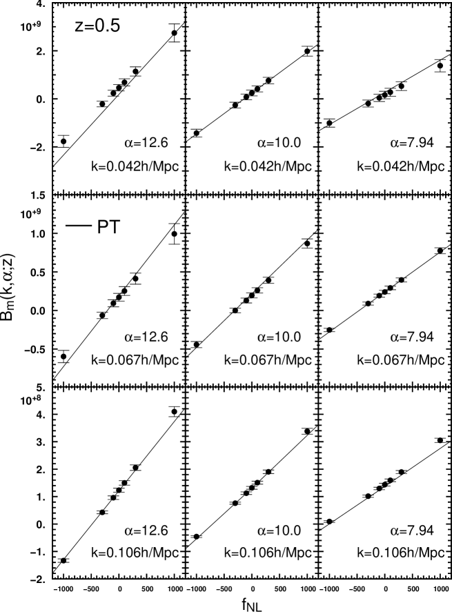
Figure 4: The matter bispectrum. Each panel shows the results for an isosceles configuration specified by $\alpha\equiv k_{1}/k_{3}$ and $k\equiv k_{1}=k_{2}$. Symbols are measurements from $N$-body simulations (the average and the standard error among different realizations) and solid lines are the perturbation theory predictions of equation (9).

5.2 halo bispectrum

We are now in a position to show the halo bispectrum. Since this is the first numerical study on the halo bispectrum in the presence of local type non-Gaussianity, it is important to understand the $N$-body results in a model-independent manner. In this subsection, we first show the $f_{\rm NL}$ dependence of the halo bispectrum. We then consider the scale dependence and compare the simulation results with the theoretical prediction of [23]. The dependence on the minimum halo mass and redshift is also investigated in section 5.2.3.

5.2.1 $f_{\rm NL}$ dependence

In order to quantitatively study the $f_{\rm NL}$ dependence of the halo bispectrum, we use all the halo catalogs with various values of $f_{\rm NL}$, and fit the measured bispectrum to the polynomial form:

$$B_{\rm h}(k,\alpha;z|f_{\rm NL})=\sum_{i=0}^{4}f_{\rm NL}^{i}B_{\rm h}^{(i)}(k,\alpha;z),$$ (19)

using the standard $\chi^{2}$ fitting with the variance of the data points measured from $N$-body simulations. For specific configurations of $(k,\alpha)$, we determine the parameters $B_{\rm h}^{(i)}$ using the halo catalogs with different values of $f_{\rm NL}$. We confirmed that the results are almost unchanged when we add higher-order polynomials with $i\geq 5$.

In Fig. 5, we show the measured bispectrum as function of $f_{\rm NL}$ for the same set of triangular configurations as plotted in Fig. 4. Note again that the value of $\alpha$ increases from right to left panels, while $k$ increases from top to bottom panels. The fitted results of Eq. (19) truncating at the first order ($i=0,1$), second order ($i=0\sim 2$) and fourth order ($i=0\sim 4$) are shown respectively as dotted, dashed and solid lines. Although we do not show the points at $f_{\rm NL}=\pm 1000$ in order to focus on more realistic values of $f_{\rm NL}$, we take account of these results when we fit the $N$-body data to Eq. (19).

The second-order term ($B_{\rm h}^{(2)}$) becomes more significant in moving from bottom to top and from right to left, and in the end, the top-left panel ($k=0.042h$Mpc^-1, $\alpha=12.6$) shows strong evidence of $B_{\rm h}^{(2)}$. Higher order terms ($B_{\rm h}^{(3)}$ and $B_{\rm h}^{(4)}$) seem to have almost no effect on the total bispectrum when $|f_{\rm NL}|\lower 2.15277pt\hbox{$\;\buildrel<\over{\sim}\;$}100$, although they may play some roles at $f_{\rm NL}=\pm 300$ (and also $\pm 1000$). This second order term, $B_{\rm h}^{(2)}$, is not seen in the matter bispectrum (Fig. 4) and we for the first time confirme that this really exists in the halo clustering in $N$-body simulations.

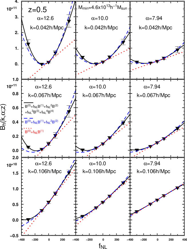
Figure 5: The halo bispectrum for some triangular configurations. Each panel shows the result for an isosceles configuration specified by $\alpha\equiv k_{1}/k_{3}$ and $k\equiv k_{1}=k_{2}$. Error bars are measurements from our simulations (the average and the standard error among different realizations) and solid lines are their $4$-th order polynomial fits, while we keep the terms up to second and linear order for dashed and dotted lines. We use the outputs at $z=0.5$ and consider the haloes more massive than $4.6\times 10^{13}h^{-1}M_{\odot}$.

5.2.2 shape and scale dependence

We next investigate the scale dependence of $B_{\rm h}^{(i)}(k,\alpha;z)$. We show them in Fig. 6 for $f_{\rm NL}=100$. The left panel shows the $\alpha$ dependence when the wave number $k$ is fixed to $0.042h$Mpc^-1, while the right panel displays the $k$ dependence when $\alpha=12.6$. The analytic prediction based on local bias (see §2 and A) predicts $B_{\rm h}^{(0)}\propto k^{2}\alpha^{0}$, $B_{\rm h}^{(1)}\propto k^{0}\alpha^{1}$ and $B_{\rm h}^{(2)}\propto k^{-2}\alpha^{3}$ in the squeezed limit at large scales ($k\to 0$, $\alpha\gg 1$), and we show these asymptotic scalings by short straight lines (normalizations are arbitrary).

The $\alpha$ dependence in the left panel is quite consistent with the theoretical predictions, and the results strongly indicate that the theoretical model captures the nature of the shape dependence. On the other hand, the $k$ dependence measured from $N$-body simulations seems different from that predicted by the theoretical model. This implies that the wave numbers shown in the figure are not sufficiently small, and the approximation used in deriving the theoretical predictions is not valid. We expect that the asymptotic scaling appears only at the scales larger than the turn over of the power spectrum (i.e., $T(k)\simeq 1$). In fact, the value of the matter transfer function at $k=0.042h$Mpc^-1, corresponding to the wavenumber at the left-most bin in the panel, is $T(k)=0.293$, and thus the approximation of $\mathcal{M}(k)\simeq\mathcal{M}_{k\to 0}\;k^{2}$ used in equation (12) cannot be applied. One can find a similar feature in Fig. 7 of Ref. [21] where the authors compute the galaxy bispectrum using one-loop perturbation theory adopting the local bias model. Although it illustrates the galaxy bispectrum for equilateral triangles, the asymptotic power law feature appears only at very large scale (i.e., $k\lower 2.15277pt\hbox{$\;\buildrel<\over{\sim}\;$}0.03h$Mpc^-1).

Nevertheless, both simulations and theory suggest that $B_{\rm h}^{(2)}>B_{\rm h}^{(1)}>B_{\rm h}^{(0)}$ at the limit of small $k$. The $B_{\rm h}^{(2)}$ term will play an important role in constraining $f_{\rm NL}$ from future surveys where we can investigate such large scales.

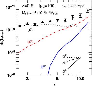
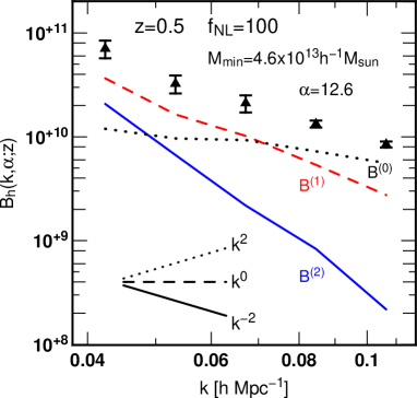
Figure 6: Shape and scale dependence of the halo bispectrum. left: $\alpha$ dependence when $k$ is fixed, right: $k$ dependence when $\alpha$ is fixed. We plot the results at $z=0.5$ for haloes more massive than $4.6\times 10^{13}h^{-1}M_{\odot}$ when $f_{\rm NL}=100$. Error bars are measurements from our simulations, while dotted, dashed and solid lines are terms which scale as $f_{\rm NL}^{0}$, $f_{\rm NL}^{1}$, and $f_{\rm NL}^{2}$, respectively. Short straight lines are corresponding analytical prediction in the squeezed limit.

5.2.3 dependence on halo mass and redshift

So far, we have concentrated on the haloes with $M_{\rm halo}\geq 4.6\times 10^{13}h^{-1}M_{\odot}$ at $z=0.5$. In this subsection, we extend our analysis to the haloes with higher mass thresholds and at different redshifts to see the dependence of the halo bispectrum on these quantities. For this purpose, we specifically consider the squeezed triangle with $k=0.042h$Mpc^-1 and $\alpha=12.6$, corresponding to the configuration shown in the top-left panel of Fig. 5, and plot in Fig. 7 the amplitude of the bispectrum against $f_{\rm NL}$ for different mass thresholds (left) and redshifts (right).

In the left hand panel, each symbol and a line respectively correspond to the measurements and the polynomial fit based on equation (19) for a fixed minimum mass of haloes given by $M_{\rm min}=4.6\times 10^{13}h^{-1}M_{\odot}$ (square/solid), $9.2\times 10^{13}h^{-1}M_{\odot}$ (triangle/dashed) and $1.4\times 10^{14}h^{-1}M_{\odot}$ (circle/dotted). Similar to Fig. 5, we can see a clear quadratic dependence on $f_{\rm NL}$, but the role of the quadratic term $B_{\rm h}^{(2)}$ seems more significant for haloes with larger minimum masses.

In the right hand panel, each symbol and line respectively show the measurements and a fit at the specific redshifts $z=0.5$ (square/solid), $1$ (triangle/dashed) and $2$ (circle/dotted). Here, we fix the minimum halo mass to $M_{\rm min}=4.6\times 10^{13}h^{-1}M_{\odot}$. Again, one can see the quadratic dependence on $f_{\rm NL}$, which become more important for higher redshifts.

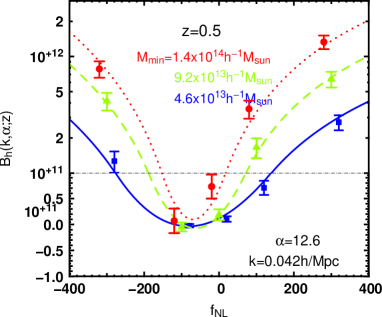
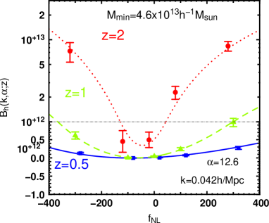
Figure 7: left: Mass dependence of the halo bispectrum at $z=0.5$. Symbols and lines are similar to Fig. 5, but we fix the triangular configuration to be the same as the top-left panel, while changing the minimum halo mass: $4.6\times 10^{13}$, $9.2\times 10^{13}$ and $1.4\times 10^{14}h^{-1}M_{\odot}$ for squares, triangles, and circles, respectively. Note that although we do not show the results for $f_{\rm NL}=\pm 1000$, we take them into account for the polynomial fitting. Note also that the vertical axis is logarithmic above the dot-dashed horizontal line, while it is linear below it. right: same as left panel but the redshift dependence for a fixed minimum halo mass ($4.6\times 10^{13}h^{-1}M_{\odot}$). Squares, triangles, and circles correspond to $z=0.5$, $1$, and $2$, respectively.

Although we do not try to find the best halo catalog or optimal weighting scheme to detect the signal of $f_{\rm NL}$ here, the balance between having denser samplings and getting higher signals for $f_{\rm NL}$ by selecting massive haloes is clearly very important. We will investigate these issues elsewhere.

6 Prospects for future survey

In this section, we discuss future prospects to detect $f_{\rm NL}$ through the measurements of the bispectrum. We especially pay attention to the importance of the higher order term, $B_{\rm g}^{(2)}$ in equation (20), which is defined in analogous to $B_{\rm h}^{(2)}$ in equation (19) that scales as $f_{\rm NL}^{2}$.

We consider three representative surveys: (i) idealistic survey with a huge volume and a deep sampling ($V=100h^{-3}$Gpc³, $n_{\rm g}=1\times 10^{-3}h^{3}$Mpc^-3, $z=1$), (ii) realistic survey with a large volume accessible in near future ($V=10h^{-3}$Gpc³, $n_{\rm g}=5\times 10^{-4}h^{3}$Mpc^-3, $z=1$), and (iii) deep survey ($V=3h^{-3}$Gpc³, $n_{\rm g}=3\times 10^{-4}h^{3}$Mpc^-3, $z=2$). Parameters of these three surveys roughly correspond to EUCLID [37], SuMIRe [38] and HETDEX [39], respectively, except for the slightly smaller value of redshift in the deep survey. Although the mass resolution of the current simulations are not sufficient to reproduce the same number density of galaxies in those surveys, it is worth giving a rough estimate of the detectability.

Under the assumption of the one-to-one correspondence between haloes and galaxies, we first estimate the minimum halo mass $M_{\rm min}$ that reproduces the mean galaxy number density, $n_{\rm g}$, for each survey. We use the mass function of [40] to derive the minimum value, $M_{\rm min}$. We then compute the linear bias parameter, $b_{1}$, using the Sheth & Tormen fit [41]. The resultant minimum masses and bias parameters are summarized in Tab. 1.

Table 1: The survey parameters used for the forecasts. We assume the one-to-one correspondence between haloes and galaxies to compute the minimum halo mass and the bias parameter from the number density.

survey	$z$	$V\,[h^{-3}$Gpc${}^{3}]$	$n_{\rm g}\,[h^{3}$Mpc${}^{-3}]$	$M_{\rm min}\,[h^{-1}M_{\odot}]$	$b_{1}$
IDEAL	$1.0$	$100$	$1\times 10^{-3}$	$2.8\times 10^{12}$	$1.9$
REALISTIC	$1.0$	$10$	$5\times 10^{-4}$	$5.0\times 10^{12}$	$2.2$
DEEP	$2.0$	$3$	$3\times 10^{-4}$	$3.4\times 10^{12}$	$3.3$

Based on our numerical experiments, we focus on the isosceles triangles with $k=0.042h$Mpc^-1 (see the left panel of Fig. 6), and model the galaxy bispectrum similar to the halo bispectrum (19) as

$${B_{\rm g}}(\alpha;z,M_{\rm min}) = B^{(0)}(z,M_{\rm min})\Bigl{[}1+f_{\rm NL}\alpha C^{(1)}(z,M_{\rm min})+f_{\rm NL}^{2}\alpha^{3}C^{(2)}(z,M_{\rm min})\Bigr{]}.$$ (20)

We estimate the coefficients, $B^{(0)}$, $C^{(1)}$ and $C^{(2)}$ from the three halo catalogs using the fitting procedure described in the previous section. We then scale them to the minimum halo masses for the three surveys as follows: for the coefficient $B^{(0)}$, we scale as $\propto b_{1}^{4}$. This is based on the fact that the term in equation (13), which scales as $b_{1}^{2}b_{2}$, is the dominant contribution at large scales, and $b_{2}\propto b_{1}^{2}$ at the high-peak limit (see B). On the other hand, we assume that $C^{(1)}$ and $C^{(2)}$ do not sensitively depend on $M_{\rm min}$ and $z$, and treat them as constants.

The left hand panel of Fig. 8 illustrates the scaling of $B^{(0)}$ measured from the $N$-body simulations. The triangles, circles and diamonds respectively correspond to the measurements from $N$-body simulations at $z=0.5$, $1$ and $2$, respectively. We also show the $\propto b_{1}^{4}$ scaling by three solid lines. The scaling seems to be a reasonable fit to the simulations. In the right hand panel, we plot $C^{(1)}$ and $C^{(2)}$ as a function of the minimum halo mass at the three redshifts (upper: $C^{(1)}$, lower: $C^{(2)}$). Since we did not detect any significant change in these coefficients for different mass and redshift, we simply derive the values of $C^{(1)}$ and $C^{(2)}$ from $\chi^{2}$ fits to the $N$-body data. We extrapolate the three coefficients to the halo masses corresponding to the three surveys. The accuracy of these scalings can only be tested using higher resolution simulations, and so leave this for future work.

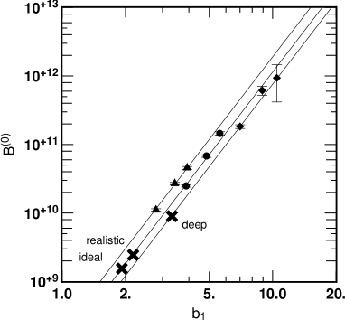
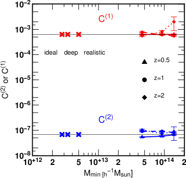
Figure 8: Scalings of the coefficients in equation (20). We assume that $B^{(0)}\propto b_{1}^{4}$, while $C^{(1)}$ and $C^{(2)}$ are treated as constants. We extrapolate these coefficients to the three surveys depicted by crosses. The triangles, circles and diamonds correspond to the measurements from $N$-body simulations at $z=0.5$, $1$ and $2$, respectively. left: $B^{(0)}$ as a function of the linear bias. right: $C^{(1)}$ and $C^{(2)}$ as a function of the minimum halo mass.

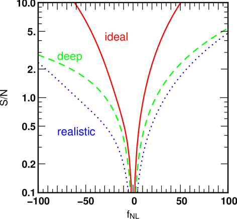
Figure 9: Signal to noise ratios from the three future surveys defined in equation (22). Notice this is estimated from only very limited configurations of Fourier space triangles: isosceles with two longer sides being $k_{1}=k_{2}=0.042h$Mpc^-1.

For statistical errors of these three surveys, we consider the Gaussian contribution as a simple estimate, and neglect the non-Gaussian error. We have [42]:

$$\left[\Delta B_{\rm g}(k_{1},k_{2},k_{3})\right]^{2}=\frac{V}{N_{\rm triangle}}\left[P_{g}(k_{1})+n_{\rm g}^{-1}\right]\left[P_{g}(k_{2})+n_{\rm g}^{-1}\right]\left[P_{g}(k_{3})+n_{\rm g}^{-1}\right],$$ (21)

where $N_{\rm triangle}$ denotes the number of independent triangular configurations in that bin, which roughly scales as $V^{2}$. We count the number of triangles for each bin, $N_{\rm triangle}$, in equation (21), assuming cubic-shaped survey with the quoted volumes. See C, where we test this formula by comparison with $N$-body simulations and show that it works reasonably well. We use the linear power spectrum for $P_{\rm g}$ assuming the bias parameters listed in Tab. 1.

Now we are in a position to discuss about the future possibility to detect the signature of the local-type primordial non-Gaussianity. In order to quantify the detectability from the $\alpha$-dependence of the bispectrum, we define the signal-to-noise ratio:

$$\left(\frac{\rm S}{\rm N}\right)^{2}\equiv\sum_{i}\frac{\left[B(k,\alpha_{i};f_{\rm NL})-B(k,\alpha_{i};f_{\rm NL}=0)\right]^{2}}{\Delta B(k,\alpha_{i};f_{\rm NL}=0)^{2}}.$$ (22)

In evaluating Eq. (22), only the isosceles triangles with $k=0.042h$Mpc^-1 are used, and the results are shown in the right hand panel of Fig. 9. It is remarkable that even with the very limited number of configurations for the bispectrum, detection of primordial non-Gaussianity is possible in all three surveys if $f_{\rm NL}$ is several dozen. This can be compared with the analysis neglecting the $B^{(2)}_{\rm g}$ term. According to [10], using the full configurations of the bispectrum leads to the constraint on $f_{\rm NL}$, $\Delta f_{\rm NL}\simeq 5-30$. Thus, we naively expected that using the full configurations taking proper account of the scale dependence of bispectrum greatly enhances the detectability of primordial non-Gaussianity, and the constraints on $f_{\rm NL}$ would be much tighter.

Finally, it is interesting to note that the $S/N$ for the deep survey depends steeply on $f_{\rm NL}$, and it exceeds that of the realistic survey of relatively large volume. This is primarily due to the $B^{(2)}_{\rm g}$ term, which scales as $f_{\rm NL}^{2}$, being more significant at higher redshift, and thus helps to detect a small non-Gaussianity. In this respect, the on-going mission BOSS [43], aiming at precisely measuring the scale of baryon acoustic oscillations from the clustering of the LRGs at $z<0.7$ and QSO absorption systems at $z\sim 2.5$, may be the promising probe for constraining or detecting primordial non-Gaussianity of local type.

7 Conclusions and Discussion

In this paper, we have studied the clustering properties of dark matter haloes from cosmological $N$-body simulations in the presence of local-type primordial non-Gaussianity. We found that the halo bispectrum measured from $N$-body simulations exhibits a strong $f_{\rm NL}$ dependence which becomes most prominent for squeezed configurations at large scales. In particular, for realistic values of $|f_{\rm NL}|\lower 2.15277pt\hbox{$\;\buildrel<\over{\sim}\;$}100$, the dependence of the halo bispectrum on $f_{\rm NL}$ is well characterized by the polynomial expansions of $f_{\rm NL}$ up to second order. Since the quadratic dependence on $f_{\rm NL}$ does not appear in the matter bispectrum at the lowest order in perturbation theory, this would be a clear indicator for the existence of primordial non-Gaussianity of the local type.

We have investigated the shape and scale dependence of the halo bispectrum arising from the $f_{\rm NL}^{2}$ term, and the simulation results are compared with theoretical predictions based on the local bias model. For the isosceles triangles characterized by $\alpha\equiv k_{1}/k_{3}$ and $k\equiv k_{1}=k_{2}$, the dependence of the halo bispectrum on $\alpha$ measured from $N$-body simulations is found to be consistent with theoretical predictions by [23]. We also examined the dependence of the halo bispectrum on minimum halo mass and redshift, and showed that the amplitude of the halo bispectrum is more significant for more massive haloes at higher redshifts.

Thus, the strong dependence of the halo/galaxy bispectrum on $\alpha$ makes the detection of primordial non-Gaussianity much more promising in future surveys. As a preliminary investigation, we have evaluated the signal-to-noise ratio for the scale dependence of the bispectrum in three representative surveys, and found that even with the very limited number of configurations of bispectrum it is possible to detect primordial non-Gaussianity if $f_{\rm NL}$ is several dozen. Thus, the detectability of primordial non-Gaussianity is expected to be greatly improved if we use all configurations of the bispectrum.

We leave the following tasks as a future work: (i) Study the effects of redshift-space distortions. Since we focus on very large scales, we expect that these effects are accurately described by linear theory, i.e., they just enhance the amplitude of the bispectrum in a scale independent way. (ii) Construct more elaborate theoretical models that are applicable to a wider range of triangular configurations and compare them with $N$-body simulations (iii) Run higher resolution simulations where we can populate haloes with galaxies and measure the galaxy bispectrum directly from simulations. These tasks are clearly very important to exploit future surveys.

Appendix A Power spectrum and bispectrum in the local bias model

In this appendix, we compute the power spectrum and bispectrum of biased tracers adopting the local bias model.

The local biasing scheme is a simple prescription to relate the galaxy/halo density field, $\delta_{\rm g}$, to matter fluctuation, $\delta_{\rm m}$, on large scales. In this treatment, the density fluctuation of galaxies/haloes smoothed over the radius $R$, $\delta_{\rm g}$, is given by a non-linear function of $\delta_{\rm m}$. On large scales, it can be expanded as

$$\delta_{\rm g}(\mbox{\boldmath$x$};R)=b_{1}\,\delta_{\rm m}(\mbox{\boldmath$x$};R)+\frac{b_{2}}{2}\,\{\delta_{\rm m}^{2}(\mbox{\boldmath$x$};R)-\sigma_{\rm R}^{2}\}+\cdots$$ (23)

with $\sigma_{\rm R}$ being $\langle\delta_{\rm m}^{2}\rangle^{1/2}$. For simplicity, we omit the dependence on redshifts throughout the appendices. Equation (23) can be rewritten in Fourier space as

$$\delta_{\rm g}(\mbox{\boldmath$k$};R) = b_{1}\delta_{\rm m}(\mbox{\boldmath$k$};R)$$ (24)

$$+\frac{1}{2}b_{2}\int\frac{d^{3}\mbox{\boldmath$q$}}{(2\pi)^{3}}\left[\delta_{\rm m}(\mbox{\boldmath$q$};R)\delta_{\rm m}(\mbox{\boldmath$k$}-\mbox{\boldmath$q$};R)-\langle\delta_{\rm m}(\mbox{\boldmath$q$};R)\delta_{\rm m}(\mbox{\boldmath$k$}-\mbox{\boldmath$q$};R)\rangle\right].$$

Using this relation, let us consider the galaxy-matter cross spectrum. With the help of perturbative expansion, a straightforward calculation yields

$$P_{\rm gm}(k;R)=b_{1}P_{\rm m}(k;R)+\frac{1}{2}b_{2}\int\frac{d^{3}\mbox{\boldmath$q$}}{(2\pi)^{3}}B_{\rm m}(q,k,|\mbox{\boldmath$k$}-\mbox{\boldmath$q$}|;R),$$ (25)

which is valid up to third order in $\delta_{\rm m}$, and the bispectrum $B_{\rm m}$ is given by the first term of equation (9). For the scales of our interest, the integration at the right-hand side of this equation can be separately done taking the large-scale limit. We then obtain [13]

$$P_{\rm gm}(k;R) = b(k,f_{\rm NL};R)P_{\rm m}(k;R)\,;$$ (26)

$$b(k,f_{\rm NL};R) = b_{1}\left\{1+2f_{\rm NL}\frac{b_{2}}{b_{1}}\frac{\sigma_{\rm R}^{2}}{\mathcal{M}_{R}(k)}\right\}.$$ (27)

Here, we define

$$\mathcal{M}_{R}(k)\equiv\mathcal{M}(k)\tilde{W}_{R}(k),$$ (28)

with $\tilde{W}_{R}$ being the Fourier transform of the window function.

The above procedure can also be applied when we calculate the galaxy auto power spectrum, $P_{\rm g}$. However, the derivation is rather simplified if we recall that the deterministic bias relation holds on large scales. Then, the auto and cross power spectra are tightly related with each other as $\{P_{\rm gm}(k;R)\}^{2}=P_{\rm g}(k;R)\,P_{\rm m}(k;R)$, which leads to

$$P_{\rm g}(k;R) = \Bigl{\{}b(k,f_{\rm NL};R)\Bigr{\}}^{2}\,P_{\rm m}(k;R)$$ (29)

$$= b_{1}^{2}\left\{1+2f_{\rm NL}\frac{b_{2}}{b_{1}}\frac{\sigma_{\rm R}^{2}}{\mathcal{M}_{R}(k)}\right\}^{2}P_{\rm m}(k;R).$$

On large scales, the effect of window functions is irrelevant, and we simply drop the subscript $R$. Introducing the bias parameter $\tilde{b}_{2}\equiv b_{2}\sigma_{\rm R}^{2}$, we finally obtain the galaxy power spectrum without smoothing:

$$P_{\rm g}(k)=b_{1}^{2}\left\{1+2f_{\rm NL}\frac{\tilde{b}_{2}}{b_{1}}\mathcal{M}^{-1}(k)\right\}^{2}P_{\rm m}(k),$$ (30)

which reproduces equation (10). In the local bias prescription, the bias parameters $b_{1}$ and $\tilde{b}_{2}$ are given just as the fitting parameters. On the other hand, in the halo and peak bias formalisms, these parameters have a specific functional form, and are related with each other. We will discuss this issue in B, and derive an explicit relation between $b_{1}$ and $\tilde{b}_{2}$ [Eq. (47)].

Next consider the galaxy bispectrum. Again, starting from equation (24), a straightforward calculation yields [23]

$$B_{\rm g}(k_{1},k_{2},k_{3};R) = b_{1}^{3}\left[B_{\rm m}(k_{1},k_{2},k_{3};R)+\frac{b_{2}}{b_{1}}\left\{P_{\rm m}(k_{1};R)P_{\rm m}(k_{2};R)+\mbox{(cyc.)}\right\}\right.$$ (31)

$$\left.+\frac{\tilde{b}_{2}}{b_{1}}B_{\rm corr}(k_{1},k_{2},k_{3};R)\right],$$

which is valid up to fourth order in $\delta_{\rm m}$. In the above, the quantities $P_{\rm m}$ and $B_{\rm m}$ are the matter power spectrum and bispectrum, whose perturbative expressions are given in equations (8) and (9). On the other hand, the term $B_{\rm corr}$ represents a new contribution arising from the matter trispectrum, $T_{\rm m}$, and it is expressed as

$$B_{\rm corr}(k_{1},k_{2},k_{3};R) \equiv \frac{1}{2\sigma_{\rm R}^{2}}\int\frac{d^{3}\mbox{\boldmath$q$}}{(2\pi)^{3}}\left[T_{\rm m}(\mbox{\boldmath$q$},\mbox{\boldmath$k$}_{1}-\mbox{\boldmath$q$},\mbox{\boldmath$k$}_{2},\mbox{\boldmath$k$}_{3};R)+\mbox{(cyc.)}\right].$$ (32)

According to the perturbative calculation by [23], the above equation can be further decomposed into several pieces as:

$$B_{\rm corr}(k_{1},k_{2},k_{3};R) = f_{\rm NL}^{2}\,B_{f_{\rm NL}^{2}}^{\rm nG}(k_{1},k_{2},k_{3};R)$$ (33)

$$+f_{\rm NL}\,\left[B_{\rm m}^{\rm nG}(k_{1},k_{2},k_{3};R)+B_{f_{\rm NL}}^{\rm nG1}(k_{1},k_{2},k_{3};R)\right.$$

$$\left.+4B_{f_{\rm NL}}^{\rm nG0}(k_{1},k_{2},k_{3};R)\sum_{i=1}^{3}\mathcal{G}_{\rm R}(k_{i})\right],$$

Here, the term $B_{f_{\rm NL}^{2}}^{\rm nG}$ comes from the leading-order trispectrum. For $k\lower 2.15277pt\hbox{$\;\buildrel<\over{\sim}\;$}0.1h$ Mpc^-1, it is approximated as

$$B_{f_{\rm NL}^{2}}^{\rm nG}(k_{1},k_{2},k_{3};R) \approx \frac{1}{2\sigma_{\rm R}^{2}}\biggl{[}8\mathcal{M}_{R}(k_{2})\mathcal{M}_{R}(k_{3})P_{\phi}(k_{1})\left[P_{\phi}(k_{2})+P_{\phi}(k_{3})\right]$$ (34)

$$\times\int\frac{d^{3}\mbox{\boldmath$q$}}{(2\pi)^{3}}\mathcal{M}_{R}(q)\mathcal{M}_{R}(|\mbox{\boldmath$k$}_{1}-\mbox{\boldmath$q$}|)P_{\phi}(q)+({\rm cyc.})$$

$$+4\mathcal{M}_{R}(k_{2})\mathcal{M}_{R}(k_{3})P_{\phi}(k_{2})P_{\phi}(k_{3})$$

$$\int\frac{d^{3}\mbox{\boldmath$q$}}{(2\pi)^{3}}\mathcal{M}_{R}(q)\mathcal{M}_{R}(|\mbox{\boldmath$k$}_{1}-\mbox{\boldmath$q$}|)$$

$$\times\left[P_{\phi}(|\mbox{\boldmath$k$}_{2}+\mbox{\boldmath$q$}|)+P_{\phi}(|\mbox{\boldmath$k$}_{3}+\mbox{\boldmath$q$}|)\right]+({\rm cyc.})\biggr{]}$$

with $P_{\phi}$ being the power spectrum of $\Phi_{\rm G}$. The explicit expressions for the other remaining terms are obtained by integrating the next-to-leading order contributions to the trispectrum. The resultant expressions become

$$B_{\rm m}^{\rm nG}(k_{1},k_{2},k_{3};R) = 4\tilde{W}_{R}(k_{1})\tilde{W}_{R}(k_{2})\tilde{W}_{R}(k_{3})\left[\frac{\mathcal{F}_{R}(k_{1})}{\mathcal{M}_{R}(k_{1})}+\frac{\mathcal{F}_{R}(k_{2})}{\mathcal{M}_{R}(k_{2})}\right]$$ (35)

$$\times P_{\rm m}(k_{1})P_{\rm m}(k_{2})F_{2}^{\rm(s)}(\mbox{\boldmath$k$}_{1},\mbox{\boldmath$k$}_{2})+({\rm cyc.}),$$

$$B_{f_{\rm NL}}^{\rm nG1}(k_{1},k_{2},k_{3};R) \approx \frac{1}{2\sigma_{\rm R}^{2}}\biggl{[}8\tilde{W}_{R}(k_{2})\tilde{W}_{R}(k_{3})P_{m}(k_{2})\mathcal{M}(k_{3})P_{\phi}(k_{3})$$ (36)

$$\times\int\frac{d^{3}q}{(2\pi)^{3}}\tilde{W}_{R}(|\mbox{\boldmath$k$}_{1}-\mbox{\boldmath$q$}|)\tilde{W}_{R}(q)\mathcal{M}(|\mbox{\boldmath$k$}_{1}-\mbox{\boldmath$q$}|)\mathcal{M}(|\mbox{\boldmath$k$}_{2}+\mbox{\boldmath$q$}|)$$

$$\times\left[P_{\phi}(|\mbox{\boldmath$k$}_{2}+\mbox{\boldmath$q$}|)+P_{\phi}(|\mbox{\boldmath$k$}_{1}-\mbox{\boldmath$q$}|)\right]F_{2}^{(s)}(-\mbox{\boldmath$k$}_{2},\mbox{\boldmath$k$}_{2}+\mbox{\boldmath$q$})$$

$$+(5~{}\mathrm{permutation})\bigg{]}.$$

The term $B^{\rm nG0}_{f_{\rm NL}}$ coincides with the first term of the matter bispectrum in equation (9). The functions ${\cal F}_{\rm R}(k_{i})$ and ${\cal G}_{\rm R}(k_{i})$ weakly depend on the smoothing scale $R$. Note that in deriving the above expressions, we have neglected the irrelevant terms at $k\lower 2.15277pt\hbox{$\;\buildrel<\over{\sim}\;$}0.1h$ Mpc^-1.

In the expression for the galaxy bispectrum, the important findings here are a new term which scales as $f_{\rm NL}^{2}$ and additional contributions which scale as $f_{\rm NL}$ to the matter bispectrum. Although [23] further considered the term arising from a cubic correction, $g_{\rm NL}\Phi_{\rm G}^{3}$ to equation (1), we do not discuss about this term in this paper. See also [17, 22, 21] for discussions about the $g_{\rm NL}$ term. Ref. [23] evaluates the asymptotic forms of each term at squeezed limit ($\alpha\gg 1$, where $k_{1}=k_{2}=\alpha k_{3}=k$) for isosceles triangular configurations, and the results are shown in equation (12) in the text. Note that Ref. [21] also compute the matter and galaxy bispectrum up to the one-loop order (i.e., $\mathcal{O}(\delta_{0}^{5})$) assuming local bias model for both local and equilateral type non-Gaussianity.

Alternatively we might be able to investigate the galaxy bispectrum using a similar description to the galaxy power spectrum:

$$B_{\rm g}(\mbox{\boldmath$k$}_{1},\mbox{\boldmath$k$}_{2},\mbox{\boldmath$k$}_{3};R) = b(k_{1},f_{\rm NL};R)\,b(k_{2},f_{\rm NL};R)\,b(k_{3},f_{\rm NL};R)\,B_{\rm m}(\mbox{\boldmath$k$}_{1},\mbox{\boldmath$k$}_{2},\mbox{\boldmath$k$}_{3};R).$$ (37)

We focus on squeezed triangles at large scales, $k\to 0$ and $\alpha\gg 1$ and drop the window function. Then we get the second-order term in $f_{\rm NL}$, which is the same as the term in equation (15) up to the prefactor. However, the coefficient of the term scaling as $f_{\rm NL}$ in this prescription is $4b_{1}^{3}+(26/7)b_{1}^{2}\tilde{b}_{2}$ in this limit, which does not reproduce the contribution that depends on the smoothing scale in equation (LABEL:eq:B1). This prescription also misses the term coming from $b_{1}^{2}b_{2}[P_{\rm m}(k_{1})P_{\rm m}(k_{2})+({\rm cyc.})]$. This implies that although some contributions are not included, this description captures the essence of the galaxy bispectrum at the squeezed limit. In other words, the $f_{\rm NL}^{2}$ term has the same origin as the scale dependent bias in the power spectrum. Although equation (37) seems rather empirical, it is naturally derived in Ref. [22], where the authors calculated the galaxy bispectrum using a multivariate biasing scheme [see their equations (73) - (76)].

Appendix B On the relation between peak biasing and local biasing models

Scale-dependence of halo power spectrum and bispectrum in the presence of primordial non-Gaussianity have been derived in the literature in different ways, based on the local bias prescription and the halo/peak formalism. However, the resultant expressions for peak and halo bias coincide with each other in the high-peak/thresold limit, and there is a clear relationship between peak bias and local bias prescriptions. The relation between the linear and quadratic bias parameter plays important roles in the accurate modelling for the power spectrum and the bispectrum of galaxies as seen in the previous appendix.

In this appendix, in order to elucidate these properties in a self-contained manner, we give an explicit relationship between the local biasing and peak biasing models, and show that the peak density field in the high-peak limit can be described by the local biasing prescription. In the end, we obtain the relation (47), which was used in Sec. 4 when comparing the $N$-body results with model prediction of halo power spectrum. We also use this relation in Sec. 6 to discuss the future detectability of the local-type primordial non-Gaussianity.

We begin by writing down the definition of peak density field. According to [24], it is given by

$$\delta_{\rm g}(\mbox{\boldmath$x$};R)=\frac{\rho_{\nu}(\mbox{\boldmath$x$};R)}{\langle\rho_{\nu}(\mbox{\boldmath$x$};R)\rangle}-1;\quad\rho_{\nu}(\mbox{\boldmath$x$};R)\equiv\Theta\Bigl{[}\delta_{\rm m}(\mbox{\boldmath$x$};R)-\nu\,\sigma_{\rm R}\Bigr{]},$$ (38)

in the Lagrangian space. In the above, $\Theta$ is the Heaviside step function and $\nu\equiv\delta_{\rm c}/\sigma_{\rm R}$ with the critical overdensity, $\delta_{\rm c}\simeq 1.686$. Strictly speaking, the above definition does not imply the local maximum of the density field, however, the local density specified above is expected to roughly correspond to the peak in the high-threshold limit, $\nu\gg 1$.

Starting with the expression (38), we want to derive Taylor series expansion of $\delta_{\rm g}$ in terms of the local density $\delta_{\rm m}$. To do this, let us first expand the peak density in terms of the Hermite polynomials:

$$\rho_{\nu}(\mbox{\boldmath$x$};R)=\sum_{n=0}^{\infty}\frac{R_{n}}{n!}\,H_{n}(\delta_{\rm m}/\sigma_{\rm R}).$$ (39)

The coefficient $R_{n}$ is given by (e.g., [44]):

$$R_{n}=\int_{-\infty}^{+\infty}\frac{dy}{\sqrt{2\pi}}\,e^{-y^{2}/2}H_{n}(y)\,\Theta\bigl{[}(y-\nu)\,\sigma_{\rm R}\bigr{]}=\left\{\begin{array}[]{ccl}{\displaystyle\frac{1}{2}\,\mbox{erfc}\left(\frac{\nu}{\sqrt{2}}\right)}&;&n=0,\\ \\ {\displaystyle\frac{e^{-\nu^{2}/2}}{\sqrt{2\pi}}H_{n-1}(\nu)}&;&n\geq 1.\end{array}\right.$$ (40)

In the high-peak limit $\nu\gg 1$, the coefficient $R_{n}$ asymptotically approaches

$$R_{n}\,\,\longrightarrow\,\,\frac{\nu^{n-1}}{\sqrt{2\pi}}\,e^{-\nu^{2}/2},$$ (41)

for $n\geq 0$. Substituting this back into (39), we obtain

$$\rho_{\nu}(\mbox{\boldmath$x$};R)\simeq\frac{e^{-\nu^{2}/2}}{\nu\sqrt{2\pi}}\,\sum_{n=0}^{\infty}\,\frac{\nu^{n}}{n!}\,H_{n}(\delta_{\rm m}/\sigma_{\rm R})=\frac{1}{\nu\sqrt{2\pi}}\,e^{-\nu^{2}+\nu(\delta_{\rm m}/\sigma_{\rm R})},$$ (42)

where we used the relation $\sum_{n}(x^{n}/n!)H_{n}(t)=e^{-x^{2}/2+t\,x}$ in the last equality. Now, recalling from the cumulant expansion theorem, $\langle e^{it\delta_{\rm m}}\rangle=\exp[\sum_{n}\,(it)^{n}\langle\delta_{\rm m}^{n}\rangle_{c}/n!]$, the averaged peak density $\langle\rho_{\nu}\rangle$ in the high-peak limit becomes

$$\bigl{\langle}\rho_{\nu}(\mbox{\boldmath$x$};R)\bigr{\rangle}\simeq\frac{e^{-\nu^{2}}}{\nu\sqrt{2\pi}}\,\,\bigl{\langle}e^{(\nu/\sigma_{\rm R})\,\delta_{\rm m}}\bigr{\rangle}=\frac{e^{-\nu^{2}}}{\nu\sqrt{2\pi}}\,\,\exp\left[\sum_{n=0}^{\infty}\,\frac{(\nu/\sigma_{\rm R})^{n}}{n!}\,\Bigl{\langle}\{\delta_{\rm m}(\mbox{\boldmath$x$};R)\}^{n}\Bigr{\rangle}_{c}\right].$$ (43)

Hence, the peak density field $\delta_{\rm g}$ becomes

$$\delta_{\rm g}(\mbox{\boldmath$x$};R)\simeq\exp\left[\frac{\nu}{\sigma_{\rm R}}\,\delta_{\rm m}(\mbox{\boldmath$x$};R)-\sum_{n=0}^{\infty}\,\frac{(\nu/\sigma_{\rm R})^{n}}{n!}\,\Bigl{\langle}\{\delta_{\rm m}(\mbox{\boldmath$x$};R)\}^{n}\Bigr{\rangle}_{c}\right]-1,$$ (44)

which can be expanded in the form of local biasing expression (23) as

$$\delta_{\rm g}(\mbox{\boldmath$x$};R)=\frac{\nu}{\sigma_{\rm R}}\,\delta_{\rm m}(\mbox{\boldmath$x$};R)+\frac{1}{2}\left(\frac{\nu}{\sigma_{\rm R}}\right)^{2}\{\delta_{\rm m}^{2}(\mbox{\boldmath$x$};R)-\sigma_{\rm R}^{2}\}+\frac{1}{3!}\left(\frac{\nu}{\sigma_{\rm R}}\right)^{3}\{\delta_{\rm m}^{3}(\mbox{\boldmath$x$};R)-\langle\delta_{\rm m}^{3}\rangle_{c}\}+\cdots.$$ (45)

Note that this expansion is done in Lagrangian space. Assuming the usual mapping from Lagrangian to Eulerian space, $b_{\rm E}=1+b_{\rm L}$, where $b_{\rm E}$ and $b_{\rm L}$ are linear bias parameters in Eulerian and Lagrangian space, the biasing parameters in the high-peak limit can be read off by comparing equation (45) with equation (23), and are expressed as

$$b_{1}=1+\frac{\nu^{2}}{\delta_{\rm c}},\quad b_{2}=\frac{\nu^{4}}{\delta_{\rm c}^{2}},\quad b_{3}=\frac{\nu^{6}}{\delta_{\rm c}^{3}},\quad\cdots.$$ (46)

Note that the higher-order biasing parameters should be also modified by the mapping from Lagrangian and Eulerian space but this effect is small in the high peaks limit and we simply ignore it. Then the biasing parameters have a relation

$$\tilde{b}_{2}=\delta_{\rm c}(b_{1}-1),$$ (47)

where $\tilde{b}_{2}=b_{2}\sigma_{\rm R}^{2}$. For a better fit of halo power spectrum (10) to the N-body simulations, a slight modification to the above relation might be necessary [see Eq. (11)].

Appendix C The Sample Variance of the Matter and Halo Bispectrum

It is of importance to investigate the variance of the bispectrum in the presence of primordial non-Gaussianity, although our simulation sets are too small to examine the full covariance of the bispectrum (see e.g., [45]; the authors performed $5000$ realizations of $(1h^{-1}$Gpc$)^{3}$ volume simulations to investigate it for Gaussian initial conditions). Here we show our measurements of the variance (i.e., the diagonal elements of the covariance matrix) for both the matter and halo bispectrum.

Fig. 10 shows the variance of the matter (left) and halo (right) bispectrum for the same configurations as in the left panel of FIg. 6 at $z=0.5$. The symbols correspond to the variance measured from $N$-body simulations, while the lines are obtained from equation (21). In computing equation (21), we substitute the value of the power spectrum measured from $N$-body simulations both for matter and halo. Overall, the analytic predictions are good approximation of the $N$-body simulations, ensuring the use of this formula. For the variance of the matter bispectrum, there is little evidence of $f_{\rm NL}$ dependence. This is natural because the matter power spectrum also depends on $f_{\rm NL}$ only weakly (see Fig. 2). On the other hand, the right panel shows a strong dependence on $f_{\rm NL}$, reflecting a strong $f_{\rm NL}$ dependence of the halo power spectrum. The prediction of equation (21) seems worse at larger $\alpha$ and larger $|f_{\rm NL}|$. Since the leading correction term to this formula have the form of $P(k_{1})T(\mbox{\boldmath$k$}_{2},\mbox{\boldmath$k$}_{3},-\mbox{\boldmath$k$}_{2},-\mbox{\boldmath$k$}_{3})+({\rm cyc.})$, this feature is quite reasonable.

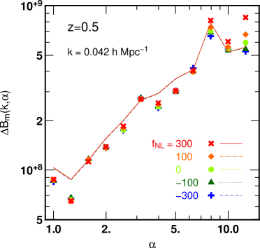
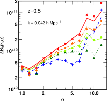
Figure 10: Variance of the matter (left) and halo (right) bispectrum. The symbols are measured from $N$-body simulations, while the lines are computed by equation (21).

References

References

- [1] Komatsu, E. et al, 2008, ApJS, 180, 330
- [2] Tegmark, M. et al. 2006, Phys.Rev.D 69, 123507
- [3] Komatsu, E., & Spergel, D. N., 2001, PRD 63, 063002
- [4] Carbone, C., Verde, L., & Matarrese, S., 2008, ApJ, 684, 1
- [5] Bartolo, N., Komatsu, E., Matarrese, S., & Riotto, A., 2004, Phys. Rep. 402, 103
- [6] [Planck Collaboration], arXiv:astro-ph/0604069
- [7] Scoccimarro, R., 2000, ApJ. 542, 1
- [8] Verde, L., Wang, L., Heavens, A. F., & Kamionkowski, M., 2000, MNRAS, 313, 141
- [9] Scoccimarro, R., Sefusatti, E., & Zaldarriaga, M., 2004, PRD, 69, 103513
- [10] Sefusatti, E., and Komatsu, E., 2007, PRD, 76, 083004
- [11] Dalal, N., Doré, O., Huterer, D., and Shirokov, A., 2008, PRD, 77, 12351
- [12] Afshordi, N., and Tolley, A. J., 2008, PRD, 78, 123507
- [13] Taruya, A., Koyama, K., & Matsubara, T., 2008, PRD, 78, 123534
- [14] Matarrese, S., and Verde, L., 2008, AJ, 677, L77
- [15] Pillepich, A., Porciani, C., and Hahn, O., 2010, MNRAS, 402, 191
- [16] Desjacques, V., Seljak, U., & Iliev, I. T., 2009, MNRAS, 396, 85
- [17] Desjacques, V., & Seljak, U., 2010, PRD, 81, 023006
- [18] Grossi, M., et al, 2009, MNRAS, 398, 321
- [19] Slosar, A., Hirata, C., Seljak, U., Ho, S., and Padmanabhan, N., 2008, JCAP, 08, 031
- [20] McDonald, P., 2008, PRD, 78, 123519
- [21] Sefusatti, E., 2009, PRD, 80, 123002
- [22] Giannantonio, T., & Porciani, C., 2010, PRD, 81, 063530
- [23] Jeong, D, & Komatsu, E., 2009, ApJ, 703, 1230
- [24] Matarrese, S., Lucchin, F., & Bonometto, S. A., 1986, ApJ, 310, 21
- [25] Fry, J. N., and Gaztanaga, E., 1993, ApJ, 413, 447
- [26] Bernardeau, F., Colombi, S., Gaztanãga, E., and Scoccimarro, R., 2002, Phys. Rep., 367, 1
- [27] Lewis, A. et al, 2000, AJ, 538, 473
- [28] Springel, V., 2005, MNRAS, 364, 1105
- [29] Taruya, A., Nishimichi, T., Saito, S., & Hiramatsu, T., 2009, PRD, 80, 123503
- [30] Nishimichi, T. et al, 2009, PASJ, 61, 321
- [31] Crocce, M., Pueblas, S., and Scoccimarro, R., 2006, MNRAS, 373, 369
- [32] LoVerde, M., Miller, A., Shandera, S., and Verde, L., 2008, JCAP, 04, 014
- [33] Matarrese, S., Verde, L., & Jimenez, R., 2000, ApJ, 541, 10
- [34] Warren, M. S., Abazajian, K., Holz, D. E., Teodoro, L., 2006, ApJ, 646, 881
- [35] Hockney, R. W, & Eastwood, J. W., 1981, Computer Simulations Using Particles (New York: McGraw-Hill)
- [36] Bartolo, N., Beltrán Almeida, J. P., Matarrese, S., Pietroni, M., & Riotto, A., 2010 JCAP, 03, 011
- [37] http://www.ias.u-psud.fr/imEuclid/
- [38] Aihara, T., talk at the IPMU international conference on dark energy: lighting up the darkness!
- [39] http://www.as.utexas.edu/hetdex/
- [40] Crocce, M., Fosalba, P., Castander, F. J., & Gaztanãga, E., 2010, MNRAS, 403, 1353
- [41] Sheth, R. K., Tormen, G., 1999, MNRAS, 308, 119
- [42] Scoccimarro, R., Colombi, S., Fry, J. N., Frieman, J. A., Hivon, Eric, & Melott, A, 1998, ApJ, 496, 586
- [43] http://cosmology.lbl.gov/BOSS/
- [44] Matsubara, T., 1995, APJS, 101, 1
- [45] Takahashi. R., et al., 2009, ApJ, 700, 479