Semiclassical dynamics and transport of the Dirac spin

Abstract

Semiclassical theory of spin dynamics and transport is formulated using the Dirac electron model. This is done by constructing a wavepacket from the positive-energy electron band, and studying its structure and center of mass motion. The wavepacket has a minimal size equal to the Compton wavelength, and has self-rotation about the average spin angular momentum, which gives rise to the spin magnetic moment. Geometric gauge structure in the center of mass motion provides a natural explanation of the spin-orbit coupling and various Yafet terms. Applications to the spin-Hall and spin-Nernst effects are discussed.

I Introduction

The electron has been playing a central role in modern science and technology. It has both a fundamental charge and spin. With the rise of spintronics, the spin degree of freedom comes to the fore as it is beginning to be employed for data processing as well as storage.spintronics Much has been learned on how to control the spin by electrical, optical as well as magnetic means. Recently, spin transport driven by thermal gradient has also been demonstrated spincalo ; xiaoxiao .

In this paper, we present a semiclassical theory of spin dynamics and transport, in order to provide an intuitive picture and effective calculation tool for such phenomena. We will focus on the Dirac model, not only because it is fundamental to the electron, but also it arises as effective theory of solid-state systems such as graphene sheetgraphene and surface of topological insulatorstopo . Therefore, this paper can serve a dual purpose: (1) to reveal the fundamental nature of the electron spin, and (2) to provide a simple setting for understanding spin related dynamics and transport phenomena in solid state systems.

The semiclassical theory is obtained by constructing a wavepacket in the positive energy electron band following the general framework of Culcer and Niuculcer . We find that the wavepacket has a minimal size equal to the Compton wavelength, and has self rotation about its average spin, much as people imagined when the spin was discovereduhlenbeck ; lorentz . The self-rotation also gives rise to the spin magnetic moment showing the fundamental orbital nature of the latter. The center of mass motion has a non-abealian geometric gauge structure, which is shown to be responsible for the spin-orbit coupling as well as various Yafet terms. This yields a spin-dependent anomalous velocity under an electric field, leading to the spin Hall effect. It also yields a spin-dependent orbital magnetization that underlies the spin Nernst effect, the spin dependent anomalous Nernst effect.

The paper is organized as follows. First we construct the wavepacket and analyze its structure and current profile. In Sec. III, we discuss the magnetic moment generated by charge circulation within the wavepacket, and study its coupling with a weak magnetic field. In Sec. IV, we derive the dynamics of the center of mass, and discuss the relation between spin-orbit coupling and geometric gauge structure. Finally, we discuss the spin Hall effect and spin Nernst effect in Sec. V based on the non-Abelian Berry curvature calculated from the Dirac theory.

II Dirac electron wavepacket

When the electron spin was first discovered from the evidence of doublets in atomic spectra, Uhlenbeck and Goudsmituhlenbeck thought it as coming from the self-rotation of the electron charge sphere. However, the idea was criticized by Lorentzlorentz , who argued that the surface of the sphere would have to rotate with a tangential speed at 137 times the speed of light to produce the accurate spin angular momentum. Ever since, we were left with no choice but to accept the spin as an abstract concept.

In 1928, Dirac formulated the Schrödinger equation for a relativistic electron.dirac The Dirac equation states

$$(-i\hbar c\mbox{\boldmath$\alpha$}\cdot\mbox{\boldmath$\nabla$}+\beta mc^{2})\Psi({\bf r},t)=i\hbar\frac{\partial}{\partial t}\Psi({\bf r},t),$$ (1)

where ${\mbox{\boldmath$\alpha$}\equiv\left(\begin{array}[]{cc}0&\mbox{\boldmath$\sigma$}\\ \mbox{\boldmath$\sigma$}&0\end{array}\right)}$ and $\beta=\left(\begin{array}[]{cc}\textrm{I}&0\\ 0&-\textrm{I}\end{array}\right)$ are $4\times 4$ matrices defined by $2\times 2$ Pauli matrices $\sigma$ and identity matrix.

The eigenenergy states are 4-component plane waves, with a two-fold degenerate positive energy branch,

$$E(q)=mc^{2}\sqrt{1+\frac{\hbar^{2}q^{2}}{m^{2}c^{2}}}\equiv\epsilon(q)mc^{2},$$ (2)

with $\hbar q=\gamma mv$ being the relativistic momentum and $\epsilon(q)=\gamma(v)=(1-v^{2}/c^{2})^{-1/2}$. There is also a two-fold degenerate branch of negative eigenenergy $-E(q)$. Dirac assumed that these states are filled to form the vacuum. A hole in this negative energy branch is identified as a positron, the antiparticle of the electron.

The 4-component plane-wave eigenstates are called Dirac spinors. They can be chosen as an orthonormal set. The two spinors for the positive energy branch are given by

$$|u_{1}({\bf q})\rangle=\sqrt{\frac{\epsilon+1}{2\epsilon}}\left[\begin{array}[]{c}1\\ 0\\ \frac{\hbar q_{z}}{mc(\epsilon+1)}\\ \frac{\lambda_{c}q_{+}}{\epsilon+1}\end{array}\right],$$ (7)

$$|u_{2}({\bf q})\rangle=\sqrt{\frac{\epsilon+1}{2\epsilon}}\left[\begin{array}[]{c}0\\ 1\\ \frac{\hbar q_{-}}{mc(\epsilon+1)}\\ \frac{-\hbar q_{z}}{mc(\epsilon+1)}\end{array}\right],$$ (12)

with $q_{\pm}=q_{x}\pm iq_{y}$. At ${\bf q}=0$, they correspond to the two spin eigenstates with $\sigma_{z}=\pm 1$.

On the other hand, the two spinors for the negative energy branch are given by

$$|u_{3}({\bf q})\rangle=\sqrt{\frac{\epsilon+1}{2\epsilon}}\left[\begin{array}[]{c}\frac{-\hbar q_{z}}{mc(\epsilon+1)}\\ \frac{-\hbar q_{+}}{mc(\epsilon+1)}\\ 1\\ 0\end{array}\right],$$ (17)

$$|u_{4}({\bf q})\rangle=\sqrt{\frac{\epsilon+1}{2\epsilon}}\left[\begin{array}[]{c}\frac{-\hbar q_{-}}{mc(\epsilon+1)}\\ \frac{\hbar q_{z}}{mc(\epsilon+1)}\\ 0\\ 1\end{array}\right].$$ (22)

In order to have intuitive picture of spin other than abstract operator in Dirac wave equation, we study its semiclassical dynamics by regarding a relativistic electron as a wavepacket, which contains only the positive energy eigenstates of the Dirac equation,

$$|w\rangle=\int d{\bf q}a({\bf q},t)e^{i{\bf q}\cdot{\bf r}}[\eta_{1}({\bf q},t)|u_{1}({\bf q})\rangle+\eta_{2}({\bf q},t)|u_{2}({\bf q})\rangle],$$ (23)

where $a({\bf q},t)=|a|e^{-i\gamma({\bf q})}$ describes the distribution of the wavepacket in momentum space. The wavepacket is sharply peaked at the charge center ${\bf q}_{c}$, and is allowed to have an overall phase $\gamma({\bf q})$. The probability amplitudes $\eta_{1}$ and $\eta_{2}$ describe the composition of the wavepacket in terms of two degenerate positive energy states with spin up and spin down. The normalization condition of the wavepacket $\langle w|w\rangle=1$ is satisfied if $\int d{\bf q}|a({\bf q},t)|^{2}=1,|\eta_{1}|^{2}+|\eta_{2}|^{2}=1.$

Now we will show that using only half of the Hilbert space, the positive energy branch, to construct the wavepacket results in a minimum size of the wavepacket. This minimum size at ${\bf q}=0$ is the Compton wavelength. To start with, we introduce a pair of projection operators, $\hat{\mathcal{P}}=|u_{1}\rangle\langle u_{1}|+|u_{2}\rangle\langle u_{2}|$ and $\hat{\mathcal{Q}}=|u_{3}\rangle\langle u_{3}|+|u_{4}\rangle\langle u_{4}|$. One can see that $\hat{\mathcal{P}}$ projects to positive energy, $\hat{\mathcal{P}}|w\rangle=|w\rangle$, $\hat{\mathcal{Q}}$ projects to negative energy, and $\hat{\mathcal{P}}+\hat{\mathcal{Q}}=1$.

The mean square radius $\Delta_{{\bf r}}$ of the wavepacket in terms of the projection operators $\hat{\mathcal{P}}$ and $\hat{\mathcal{Q}}$ is,

$$\Delta_{{\bf r}}^{2} \equiv \langle w|{\bf r}^{2}|w\rangle-\langle w|{\bf r}|w\rangle^{2}$$ (24)

$$= \langle w|{\bf r}(\hat{\mathcal{P}}+\hat{\mathcal{Q}}){\bf r}|w\rangle-\langle w|{\bf r}|w\rangle^{2}$$ (25)

$$= \langle w|{\bf r}\hat{\mathcal{P}}{\bf r}|w\rangle-\langle w|{\bf r}|w\rangle^{2}+\langle w|{\bf r}\hat{\mathcal{Q}}{\bf r}|w\rangle$$ (26)

$$= \Delta_{\hat{\mathcal{P}}{\bf r}\hat{\mathcal{P}}}^{2}+\langle w|{\bf r}\hat{\mathcal{Q}}{\bf r}|w\rangle.$$ (27)

$\Delta_{\hat{\mathcal{P}}{\bf r}\hat{\mathcal{P}}}$ is the mean square radius of the projected position operator $\hat{\mathcal{P}}{\bf r}\hat{\mathcal{P}}$, and is a positive-definite quantity. The second term is calculated as follows :

$$\langle w|{\bf r}\hat{\mathcal{Q}}{\bf r}|w\rangle$$ (28)

$$= \left(\frac{\lambda_{c}}{2\epsilon(q_{c})}\right)^{2}\left|\bar{\mbox{\boldmath$\sigma$}}-\frac{\lambda_{c}^{2}}{\epsilon(q_{c})[\epsilon(q_{c})+1]}{\bf q}_{c}({\bf q}_{c}\cdot\bar{\mbox{\boldmath$\sigma$}})\right|^{2},$$ (29)

where we have used the relation between the matrix element of position operator and velocity operator. $\bar{\mbox{\boldmath$\sigma$}}\equiv\eta_{{\alpha}}^{\dagger}\mbox{\boldmath$\sigma$}\eta_{{\alpha}}$ is the spinor-averaged spin with $\eta_{{\alpha}}=\left(\begin{array}[]{c}\eta_{1}\\ \eta_{2}\end{array}\right)$, and $\lambda_{c}=\frac{\hbar}{mc}$ is the Compton wavelength.

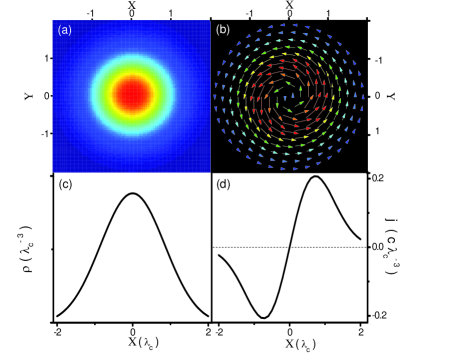
Figure 1: (Color online) Distribution of (a) probability density and (b) probability current density of the wavepacket with a Gaussian distribution $a({\bf q},t)$. The length scale is in units of the Compton wavelength $\lambda_{c}$ and the color bar is from high density (red) to low density (blue). The profiles of (a) and (b) along the $x$-axis are plotted in (c) and (d).

Thus, we obtain the lower bound of the mean square wavepacket radius as $\langle w|{\bf r}\hat{\mathcal{Q}}{\bf r}|w\rangle^{1/2}$. At $q_{c}=0$, it reduces to half of the Compton wavelength. We may regard this as the minimum intrinsic radius of the electron wavepacket. This minimum size is a consequence of using only half of the Hilbert space in constructing an electron wavepacket and it is 137 times larger than the classical electron radius used in Lorentz’s argument.lorentz Therefore, even for the tightest possible electron wavepacket, the electron does not have to rotate faster than the speed of light. To probe the wavepacket at length scales smaller than the Compton wavelength, the negative energy branch has to be involved.

In Fig. 1, we plot the probability density, probability current density of a wavepacket, which are defined as $\rho({\bf r})=w^{\dagger}({\bf r})w({\bf r})$ and ${\bf j}({\bf r})=w^{\dagger}({\bf r})c\mbox{\boldmath$\alpha$}w({\bf r})$. The electron wavepacket is spin up (in the $\hat{z}$ direction) and has a Gaussian distribution $a({\bf q})$ in momentum space with zero mean momentum ($q_{c}=0$). A circulating current around the spin axis is clearly seen in Fig.1b, with maxima at $r=\lambda_{c}$. In Fig. 2, the current density of the wavepacket shows a rotating velocity profile, ${\bf v}({\bf r})={\bf j}({\bf r})/\rho({\bf r})$, much like that of a rigid sphere (goes linearly with the radius), except that beyond the edge it gradually saturates to the speed of light. This implies a rigid core inside the self-rotating wavepacket. A classical analogy of this is a uniformly charged, self-rotating sphere, with a diameter of the Compton wavelength, which is exactly the spinning ball picture of Uhlenbeck and Goudsmit.uhlenbeck

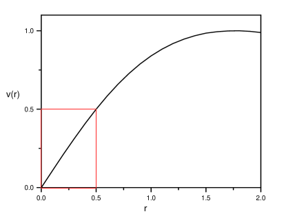
Figure 2: Velocity distribution ${\bf v}({\bf r})$ (in units of c) of a rotating wavepacket. The distance $r$ (in units of the Compton wavelength $\lambda_{c}$) measures from the center of charge. The figure shows the rotating wavepacket has a rigid core with a diameter equals to the Compton wavelength.

III The spin magnetic moment

The current circulating around the spin axis of the wavepacket would generate a magnetic moment ${\bf M}=\frac{-e}{2}\int d{\bf r}({\bf r}-{\bf r}_{c})\times{\bf j}({\bf r})$ where ${\bf r}_{c}=\langle w|{\bf r}|w\rangle$ is the center of the wavepacket. With some algebra, one can show that

$${\bf M} = \frac{-e}{2}\langle w|({\bf r}-{\bf r}_{c})\times{\bf v}|w\rangle$$ (30)

$$= \frac{-e}{2}\sum_{{{\alpha\beta}}}\eta^{*}_{\alpha}(\textbf{q})\mbox{\boldmath${\cal R}$}_{{{\alpha\beta}}}\times{\bf v}_{{{\beta\alpha}}}\eta_{\alpha}(\textbf{q}),$$ (31)

expressed in terms of the matrix element of the velocity operator ${\bf v}_{{\alpha\beta}}=\langle u_{{\alpha}}|c\mbox{\boldmath$\alpha$}|u_{{\beta}}\rangle$, and the so-called Berry connection $\mbox{\boldmath${\cal R}$}_{{\alpha\beta}}=\langle u_{{\alpha}}|i\frac{\partial}{\partial{\bf q}}|u_{{\beta}}\rangle$.

After putting in the velocity operator ${\bf v}=c\mbox{\boldmath$\alpha$}$ in calculation, we obtain

$${\bf M}=\frac{-e\hbar}{2m\epsilon^{2}(q_{c})}\left[\bar{\mbox{\boldmath$\sigma$}}+\lambda_{c}^{2}\frac{{\bf q_{c}\cdot{\bar{\mbox{\boldmath$\sigma$}}}}}{\epsilon(q_{c})+1}{\bf q}_{c}\right],$$ (32)

where $\bar{\mbox{\boldmath$\sigma$}}=\eta_{{\alpha}}^{\dagger}\mbox{\boldmath$\sigma$}\eta_{{\alpha}}$ is the spinor-average spin. At ${\bf q}_{c}=0$, it reproduces the classical result, ${\bf M}=-\frac{e\hbar}{2m}\bar{\mbox{\boldmath$\sigma$}}=-\mu_{B}\bar{\mbox{\boldmath$\sigma$}}$, with the Bohr magneton being $\mu_{B}=\frac{e\hbar}{2m}$.

In the following, we will show that the magnetic moment induced by the charge circulation is characterized not by the canonical angular momentum but by the spin.

The canonical angular momentum operator is defined as ${\bf L}=m{\bf r}\times{\bf p}=m{\bf r}\times\frac{\hbar}{i}\nabla$. Unlike the momentum ${\bf p}$, the canonical angular momentum is not a conserved quantity, $d{\bf L}/dt\neq 0$. It is the total angular momentum ${\bf J}={\bf L}+{\bf S}$ that is conserved. For a self-rotating Dirac wavepacket, the canonical angular momentum is zero (when the momentum operator ${\bf p}$ acts on the wavefunction $|w\rangle$, it gives $\hbar{\bf q}$, and the matrix element ${\bf q}_{\alpha\beta}=0$ implies ${\bf L}=\langle w|({\bf r}-{\bf r}_{c})\times{\bf p}|w\rangle=0$).

In Dirac theory, spin is represented as a $4\times 4$ matrix, ${\mbox{\boldmath$\Sigma$}}=\frac{1}{2}\left(\begin{array}[]{cc}\mbox{\boldmath$\sigma$}&0\\ 0&\mbox{\boldmath$\sigma$}\end{array}\right).$ We can obtain the average spin by calculating the expectation value of the spin operator,

$$\bar{\mbox{\boldmath$\Sigma$}} = \langle w|\mbox{\boldmath$\Sigma$}|w\rangle=\sum_{{{\alpha\beta}}}\eta^{*}_{\alpha}(\textbf{q})\Sigma_{\alpha\beta}\eta_{\beta}(\textbf{q})$$ (33)

$$= \frac{1}{2\epsilon(q_{c})}\left[\bar{\mbox{\boldmath$\sigma$}}+\lambda_{c}^{2}\frac{{\bf q_{c}\cdot{\bar{\mbox{\boldmath$\sigma$}}}}}{\epsilon(q_{c})+1}{\bf q}_{c}\right],$$ (34)

where $\Sigma_{\alpha\beta}=\langle u_{\alpha}|\mbox{\boldmath$\Sigma$}|u_{\beta}\rangle$. It is remarkable that the average spin calculated from the abstract spin operator has the same structure (inside the square bracket of Eq.(32)) as the orbital magnetic moment obtained semiclassically. We can therefore relate these two quantities by

$${\bf M}=-g\frac{e\hbar}{2m\epsilon(q_{c})}\bar{\mbox{\boldmath$\Sigma$}},$$ (35)

where the $g$-factor is 2. Note that the $\epsilon$ in the denominator can be absorbed in the relativistic mass to form the relativistic Bohr magneton $\mu_{B}=e\hbar/2m\epsilon(q_{c})$. With ${\bf q}_{c}=0$, ${\bf M}=-g\mu_{B}\bar{\mbox{\boldmath$\Sigma$}}$.

The spin therefore can be thought of as coming from the charge circulation of the electron wavepacket. In fact, the spin is related to the mechanical angular momentum (the mass circulation current), ${\bf L}_{mech}=m\langle w|({\bf r}-{\bf r}_{c})\times{\bf v}|w\rangle=2\hbar\bar{\mbox{\boldmath$\Sigma$}}$. The g-factor of 2 is then explained by the fact that the mechanical angular momentum calculated from the mass circulating current, which is proportional to the charge circulating current, is twice of the spin expectation value. In a semiconductor, the g-factor can deviate from 2 dramatically.gfactor The origin of the anomalous g-factor can be explained as the same way coming from the self rotation of electron wavepacket.mcreview

In the past, there has been a number of attempts to find an intuitive understanding of the spin magnetic moment within the framework of the Dirac theory. Huang huang suggested that it can be thought of as the current produced by the zitterbewegung zitter . Ohanian ohenian showed that the electron spin magnetic moment originates from a circulating flow of energy of the wave field based on an earlier idea of Belinfante Bel . These ideas are similar in spirits with Uhlenbeck and Goudsmit’s picture of the spin. Here, we see that the rotating charge model can indeed be re-established explicitly and firmly within the wavepacket formulation.

The magnetic moment obtained above exists even in the absence of a magnetic field. We will show that in the existence of an external magnetic field, the magnetic moment, coming from the self-rotation of the wavepacket, causes an energy shift in its total energy, the Zeeman energy.

First we assume the external field is weak and varying on a length scale much larger than that of the wavepacket. This requirement allows us to expand the local Hamiltonian around the position of the charge center ${\bf r}_{c}$ to the first order of the gradient correction, $\hat{H}({\bf r}_{c},{\bf q}_{c},t)=\hat{H}_{0}({\bf r}_{c},{\bf q}_{c},t)+({\bf r}-{\bf r}_{c})\cdot(\partial\hat{H}/\partial{\bf r}_{c}).$ For a uniform magnetic field ${\bf B}=\nabla\times{\bf A}({\bf r}_{c},t)$, with a symmetric vector potential ${\bf A}({\bf r},t)=\frac{1}{2}{\bf B}\times{\bf r}$, we have $\hat{H}_{0}({\bf r}_{c},{\bf k}_{c},t)=c\mbox{\boldmath$\alpha$}\cdot\hbar{\bf k}_{c}+\beta mc^{2}$, where ${\bf k}_{c}={\bf q}_{c}+\frac{e}{\hbar}{\bf A}({\bf r}_{c},t)$ is the kinetic momentum. The energy correction due to the external field is given by

$$\delta E = \left\langle w\left|{({\bf r}-\bf r}_{c})\cdot\partial\hat{H}/\partial{\bf r}_{c}\right|w\right\rangle$$ (36)

$$= \left\langle w|\Sigma_{i,j}(r_{i}-r_{c,i})e\partial A_{j}/\partial r_{i}|w\right\rangle=-{\bf M}\cdot{\bf B},$$ (37)

We therefore observe that the Zeeman energy comes from the energy gradient correction and is associated with the ${\bf M}$ defined in Eq.(31).

When both the electric field $\bf{E}$ and magnetic field $\bf{B}$ are present, the total energy of a wavepacket is

$$E({\bf r}_{c},{\bf k}_{c})=\langle w|\hat{H}|w\rangle=E_{0}({\bf k}_{c})-e\phi({\bf r}_{c})-{\bf M}\cdot{\bf B},$$ (38)

where $E_{0}({\bf k}_{c})$ is given by Eq. (2) with $q_{c}\rightarrow k_{c}$, and $\phi({\bf r}_{c})$ is the scalar potential of the electric field.

IV The dynamics of the wavepacket

Surprisingly, there are no spin-orbit coupling in the wavepacket energy (Eq. (38)), which is expected to appear at the first order of the electric field. One can quantize the semiclassical Dirac electron and show that the spin-orbit coupling is related to the non-canonical wavepacket dynamics.mcreview ; bliokh ; berard ; xiao The effective Lagrangian of a wavepacket is culcer ,

$$\mbox{\boldmath${\cal L}$}=i\hbar\eta^{\dagger}\frac{\partial\eta}{\partial t}+\hbar\dot{\textbf{k}}_{c}\cdot\mbox{\boldmath${\cal R}$}+\hbar\textbf{k}_{c}\cdot{\dot{\textbf{r}}_{c}}-\frac{e}{c}\textbf{A}\cdot{\dot{\textbf{r}}_{c}}-E(\textbf{r}_{c},\textbf{k}_{c}).$$ (39)

For a Dirac electron, the Berry connection is $\mbox{\boldmath${\cal R}$}=\frac{\lambda_{c}^{2}}{2\epsilon(\epsilon+1)}\textbf{ k}_{c}\times{{\mbox{\boldmath$\sigma$}}}.$

From the Lagrangian, one can derive the equations of motion for the centers of charge position and momentum, correct to linear order in fields,

$$\hbar\dot{\textbf{k}}_{c} = -e\textbf{E}-\frac{e}{c}\frac{\hbar\textbf{ k}_{c}}{\epsilon m}\times\textbf{B},$$ (40)

$$\dot{\textbf{r}}_{c} = \frac{\hbar\textbf{k}_{c}}{\epsilon m}+\frac{e}{\hbar}\left(\textbf{E}\times\textbf{F}+\textbf{ B}\cdot\textbf{F}\frac{{\hbar\textbf{k}_{c}}}{\epsilon mc}\right),$$ (41)

where $\textbf{F}=\langle\mbox{\boldmath${\cal F}$}\rangle=\eta_{\alpha}^{\dagger}\mbox{\boldmath${\cal F}$}\eta_{\alpha}$, $\mbox{\boldmath${\cal F}$}=-\frac{\lambda_{c}^{2}}{2\epsilon^{3}}\left(\mbox{\boldmath$\sigma$}+\lambda_{c}^{2}\frac{\textbf{ k}_{c}\cdot\mbox{\boldmath$\sigma$}}{\epsilon+1}\textbf{ k}_{c}\right)$ is called the Berry curvature.

The equation for spin precession is given by

$$\dot{\bar{\mbox{\boldmath$\sigma$}}}=(\lambda_{c}/\epsilon)(e/\hbar)\left[\textbf{B}+(\lambda_{c}/(\epsilon+1))\textbf{E}\times\textbf{k}_{c}\right]\times\bar{\mbox{\boldmath$\sigma$}},$$ (42)

which agrees with the Bargmann-Michel-Telegdi equationbmt .

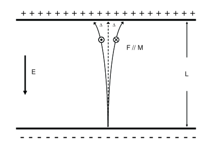
Figure 3: Electrons are accelerated by a static electric field in a parallel plate capacitor. Magnetic moment M points into (out of) the page, giving rise to an anomalous velocity to the right (left). The trajectory shift is $\Delta=\lambda_{c}\sqrt{eV_{0}/2mc^{2}}$ with a potential difference $V_{0}=EL$.

When only the electric field exists ($\textbf{B}=0$ in Eq. (41)), we find that the wavepacket has an anomalous velocity in the direction of ${\bf E}\times{\bf F}$, and since $\mbox{\boldmath${\cal F}$}\propto\mbox{\boldmath$\sigma$}$ at low velocity, spin-up and spin-down electrons would have opposite transverse velocities (see Fig. 3).

Notice that the $\textbf{r}_{c}$ and $\textbf{k}_{c}$ in Eq. (14) are not a canonical pair, due to the presence of the gauge potentials ${\cal R}$ and A. Their connections with canonical variables ${\bf r}$ and ${\bf p}$ are given by (valid in weak fields), mcreview

$$\textbf{r}_{c} = \textbf{r}+\mbox{\boldmath${\cal R}$}(\mbox{\boldmath$\pi$})+\mbox{\boldmath${\cal G}$}(\textbf{k}_{c})(\mbox{\boldmath$\pi$}),$$

$$\hbar\textbf{k}_{c} = \mbox{\boldmath$\pi$}+\frac{e}{c}\textbf{ B}\times\mbox{\boldmath${\cal R}$}(\mbox{\boldmath$\pi$}),$$ (43)

where $\mbox{\boldmath$\pi$}=\textbf{p}+\frac{e}{c}\textbf{A}(\textbf{ r})$, and $\mbox{\boldmath${\cal G}$}_{\alpha}\equiv 1/2(\partial\mbox{\boldmath${\cal R}$}/\partial k^{\alpha})\cdot(\mbox{\boldmath${\cal R}$}\times\textbf{B})$. This is analogous to the Peierls substitution for the momentum.

Now we can re-quantize the semiclassical Dirac energy Eq. (38) and obtain the relativistic Pauli Hamiltonian for all orders of velocitysilenko ,

$${H}(\textbf{r},\textbf{p})=\epsilon({\pi})mc^{2}-e\phi(\textbf{r})+\frac{\mu_{B}}{\epsilon}\mbox{\boldmath$\sigma$}\cdot\left[\frac{\textbf{E}\times\mbox{\boldmath$\pi$}}{(\epsilon+1)mc}+\textbf{B}\right]$$ (44)

This alternative approach is intuitive when compared to formal procedures of block-diagonalization, such as the Foldy-Wouthuysen transformation.foldy

In Eq. (44), the third term is the spin-orbit coupling which emerges from the first-order gradient expansion of the scalar potential, $\partial\phi/\partial\textbf{r}\cdot\mbox{\boldmath${\cal R}$}$. In the literature, $-e\mbox{\boldmath${\cal R}$}$ has often been called an electric dipole which couples to the electric field to give rise to the spin-orbit energymathur . For electrons in narrow gap semiconductors, the spin-orbit coupling is called a Yafet termyafet . This is unfortunately artificial, because its existence depends on the unphysical position r which depends on the choice of the SU(2) gauge, instead of the true position $\textbf{r}_{c}$. The equations of motion based on the Pauli Hamiltonian is consistent with the Dirac theory if and only if one recognizes this fact.

V Spin Hall Effect and Spin Nernst Effect

The presence of the Berry curvature gives the Dirac electron a tiny but nonzero anomalous velocity in the vacuum. Similar to the electron in semiconductor, such a Berry curvature would lead to the spin Hall effect and the spin Nernst effect. The discussion below relies on the formulation developed previously for the Hall effect and the Nernst effect for spinless electrons.xiao But their results are strictly applicable to the present case as long as the electron spin is conserved.

For spinless electrons, the Hall conductivity is given by

$$\sigma_{xy}=-\frac{e^{2}}{\hbar}\int\frac{d^{3}k}{(2\pi)^{3}}f({\bf k})\Omega_{z}({\bf k}),$$ (45)

where $f({\bf k})$ is the Fermi distribution function in equilibrium, $\Omega_{z}({\bf k})$ is the Abelian Berry curvature. The Nernst current perpendicular to the temperature gradient is given by $j_{x}=\alpha_{xy}(-\nabla_{y}T)$, and the Nernst coefficient $\alpha_{xy}$ is related to the Hall conductivity $\sigma_{xy}$ via

$$\alpha_{xy}=\frac{1}{e}\int dE\left(-\frac{\partial f}{\partial E}\right)\sigma_{xy}(E)\frac{E-\mu}{T},$$ (46)

where $\sigma_{xy}(E)$ is the Hall conductivity from all of the states below energy $E$ and $\mu$ is the chemical potential.

For electrons with spins, we need to replace the Abelian Berry curvature $\Omega_{z}$ in Eq. (45) by the non-Abelian one averaged over spin, $\langle{\cal F}_{z}\rangle$. For a Dirac electron, in the limit of $\hbar k<<mc$, we have ${\cal F}_{z}=-(\lambda_{c}^{2}/2)\sigma_{z}$. For a Dirac electron gas that is not spin-polarized, the spin-averaged $\langle{\cal F}_{z}\rangle$ is zero, even though ${\cal F}_{z}$ itself is non-zero. As a result, one expects neither charge Hall effect nor Nernst effect.

If the electron gas is spin polarized, then $\langle{\cal F}_{z}\rangle$ is not zero and one has the anomalous Hall effect (see Eq. (45)). At the mean time, according to Eq. (46), there is an anomalous Nernst effect. Again in the small momentum limit, we have

$$\sigma_{xy}\simeq\frac{e^{2}}{\hbar}\frac{\lambda_{c}^{2}}{2}\frac{n}{2}\langle\sigma_{z}\rangle,$$ (47)

where $n$ is the electron density.

At low temperature (compared to the Fermi temperature), the Nernst coefficient and the Hall coefficient are related by the Mott relation (which can be derived from Eq. (46)),

$$\alpha_{xy}\simeq\frac{\pi^{2}}{3}\frac{k_{B}^{2}T}{e}\frac{d\sigma_{xy}}{d\mu}.$$ (48)

Therefore, $\alpha_{xy}$ is proportional to the density of states at the Fermi level, $dn/d\mu$.

Since the Berry curvature ${\cal F}_{z}\propto\sigma_{z}$ at low velocity, spin-up and spin-down electrons would move to opposite transverse directions. Therefore, even if the electron gas is not spin polarized, there can still be a spin Hall effect (see Fig.3). This is analogous to the emergence of the spin Hall effect in bulk (non-magnetic) semiconductors.murakami

The spin Hall conductivity is given as (valid when electron spin is conserved),

$$\sigma^{z}_{xy}=\frac{e}{2}\int\frac{d^{3}k}{(2\pi)^{3}}f({\bf k})\langle\sigma_{z}{\cal F}_{z}\rangle,$$ (49)

which is approximately equal to $(e/2)(\lambda_{c}^{2}/2)(n/2)$. Similarly, the spin Nernst coefficient is given by

$$\alpha^{z}_{xy}\simeq\frac{\pi^{2}}{3}\frac{k_{B}^{2}T}{e}\frac{d\sigma^{z}_{xy}}{d\mu}.$$ (50)

For Fermi gas at low temperature, we have $\sigma^{z}_{xy}=\frac{ek_{F}^{3}\lambda_{c}^{2}}{24\pi^{2}}$ and $\alpha^{z}_{xy}\simeq\frac{k_{B}^{2}k_{F}^{2}\lambda_{c}^{2}}{24}T$. For electrons in semiconductor, the Berry curvature has the same structure as in vacuum but with different coefficient, i.e. ${\cal F}_{z}=\frac{2V^{2}}{3}[\frac{1}{E_{g}^{2}}-\frac{1}{(E_{g}+\Delta)^{2}}]\sigma_{z}$, therefore the effect can be enlarged by a factor $\frac{4V^{2}}{3\lambda_{c}^{2}}[\frac{1}{E_{g}^{2}}-\frac{1}{(E_{g}+\Delta)^{2}}]$, where $E_{g}$ is the energy gap between conduction band and top valence band, and $\Delta$ is energy separation between the split-off band and top valence band. For example, in GaAs with $E_{g}=1.424$eV, $\Delta=0.34$eV, $E_{p}=2m_{e}V^{2}/\hbar^{2}=22.7$eV, the effect is enlarged by $1.3\times 10^{6}$ times. Similar to the anomalous Nernst effect, such a contribution is ultimately originated from the Berry phase correction to (now spin-dependent) orbital magnetization.xiao

VI Conclusion

We have shown that a self-rotation picture of the wavepacket explains the origin of the electron spin by regarding the non-relativistic electron as a wavepacket at the bottom of the positive energy branch of the Dirac theory. The minimum size of the wavepacket equals to the Compton wavelength. The magnetic moment generated from the circulating charge current gives the Bohr magneton in non-relativistic limit, and is responsible for the Zeeman energy under the external fields. The g-factor of 2 comes from the fact that the mechanical angular momentum from the mass circulating current is twice of the spin expectation value. The spin-orbit coupling emerges from the first-order gradient expansion of the scalar potential and is related to the Berry connection. Finally, the Berry curvature plays an important role in both the spin Hall effect and the spin Nernst effect. Although the predictions of our semiclassical theory can be calculated from the microscopic Dirac theory, it provides not only an intuitive conceptual view but also a quantitatively accurate theoretical framework. The method can be directly transplanted to Bloch electrons in crystals, making predictions on various thermodynamics as well as transport phenomena, such as spin Nernst effect discussed specifically in this paper.

The authors would like to thank E. I. Rashba, M. Stone, L. Balent, D. Culcer, and D. Xiao for many helpful discussions.

References

- (1) G. A. Prinz, Science 282, 1660 (1998); S. A. Wolf et al., Science 294, 1488 (2001).
- (2) M. Hatami, G. E.W. Bauer, Q. Zhang ,and P. J. Kelly, Physical Review Letter 99, 066603-1 (2007)
- (3) D. Xiao, Y. Yao, Z. Fang, and Q. Niu, Phys. Rev. Lett. 97, 026603 (2006).
- (4) C. L. Kane and E. J. Mele, Phys. Rev. Lett. 95, 226801 (2005); Y.W. Son, M. L. Cohen and S. G. Louie, Phys. Rev. Lett 97 216803 (2006); S. Y. Zhou et al, Nature Mater. 6 770 (2007)
- (5) B. A. Bernevig et al, Science 314, 1757 (2006); Y.-Q. Xia et al. Nature Phys. 5, 398 (2009); H. Zhang et al. Nature Phys. 5, 438 (2009).
- (6) D. Culcer, Y. Yao, and Q. Niu, Phys. Rev. B 72, 085110 (2005).
- (7) G. Uhlenbeck and S. Goudsmit Naturwissenschaften 13 953 (1925); G. Uhlenbeck and S. Goudsmit, Nature 117, 264 (1926). Same idea was proposed by R. deL. Kronig one year earlier, see Kronig R. deL. Kronig Nature 117, 550 (1926).
- (8) The discovery of the electron spin, the lecture was deliveried by S. Goudsmit in 1971 at Dutch, and translated by J. H. van der Waals. See also Sin-itiro Tomonaga, The story of the spin, lecture two (The Univ. of Chicago press, 1997)
- (9) P.A.M. Dirac, Proc. Roy. Soc. A 117, 610 (1928); ibid, 118, 351 (1928).
- (10) L. M. Roth, B. Lax, and S. Zwerdling, Phys. Rev. 114, 90 (1959).
- (11) M.C. Chang and Q. Niu, J. Phys.: Condens. Matter 20 (2008) 193202 (17pp).
- (12) K. Huang, Am. J. Phys. 20, 479-484 (1952).
- (13) E. Schrödinger, Sitzber. preuss. Akad. Wiss., Physikmath. Kl. 24, 418 (1930); E. Schrödinger, Ürber die kräftefreie Bewegung in der relativistischen Quantenmechanik (“On the free movement in relativistic quantum mechanics”), Berliner Ber., pp. 418-428 (1930); Zur Quantendynamik des Elektrons, Berliner Ber, pp. 63-72 (1931)
- (14) H. C. Ohanian, Am. J. Phys. 54(6), 500 (1986).
- (15) Belinfante, Physica 6, 887 (1939)
- (16) K. Yu. Bliokh, Europhys. Lett. 72, 7 (2005).
- (17) A. Bérard and H. Mohrbach, Phys. Lett. A 352, 190 (2006)
- (18) D. Xiao, J. Shi, and Q. Niu, Phys. Rev. Lett. 95, 137204 (2005).
- (19) A. J. Silenko, J. Math. Phys. 44, 2952 (2003).
- (20) V. Bargmann, L. Michel, and V.L. Telegdi, Phys. Rev. Lett. 2, 435 (1959).
- (21) L. Foldy and S. Wouthuysen, Phys. Rev. 78, 29 (1950).
- (22) H. Mathur, Phys. Rev. Lett. 67, 3325 (1991); R. Shankar and H. Mathur, Phys. Rev. Lett. 73, 1565 (1994). Also see R.G. Littlejohn and W.G. Flynn, Phys. Rev. A 45, 7697 (1992).
- (23) Y. Yafet, in Solid State Physics, edited by F. Seitz and D. Turnbull (Academic Press, Inc., New York, 1963), Vol. 14.
- (24) S. Murakami, N. Nagaosa, and S.C. Zhang, Science 301, 1348 (2003).