Abstract

A MIMO radar system is proposed for obtaining angle and Doppler information on potential targets. Transmitters and receivers are nodes of a small scale wireless network and are assumed to be randomly scattered on a disk. The transmit nodes transmit uncorrelated waveforms. Each receive node applies compressive sampling to the received signal to obtain a small number of samples, which the node subsequently forwards to a fusion center. Assuming that the targets are sparsely located in the angle-Doppler space, based on the samples forwarded by the receive nodes the fusion center formulates an $\ell_{1}$-optimization problem, the solution of which yields target angle and Doppler information. The proposed approach achieves the superior resolution of MIMO radar with far fewer samples than required by other approaches. This implies power savings during the communication phase between the receive nodes and the fusion center. Performance in the presence of a jammer is analyzed for the case of slowly moving targets. Issues related to forming the basis matrix that spans the angle-Doppler space, and for selecting a grid for that space are discussed. Extensive simulation results are provided to demonstrate the performance of the proposed approach at difference jammer and noise levels.

Keywords: Compressive sampling, MIMO Radar, DOA estimation, Doppler estimation

I Introduction

Multiple-input multiple-output (MIMO) radar systems have received considerable recent attention, e.g., [1]-[3]. Unlike a conventional transmit beamforming radar system that uses highly correlated waveforms, a MIMO radar system transmits multiple independent waveforms via its antennas. A MIMO radar system is advantageous in two different scenarios [4]-[6]. In the first one [4], the transmit antennas are located far apart from each other relative to their distance to the target. This enables the radar to view the target from different directions simultaneously. The MIMO radar system transmits independent probing signals from decorrelated transmitters through different paths, and thus each target return carries independent information about the target. Combining these independent target returns results in a diversity gain, which enables the MIMO radar system to reduce target radar cross section (RCS) scintillations and achieve high target resolution. In the second scenario [5], a MIMO radar is equipped with $M_{t}$ transmit and $N_{r}$ receive antennas that are close to each other relative to the target, so that the RCS does not vary between the different paths. In this scenario, the phase differences induced by transmit and receive antennas can be exploited to form a long virtual array with $M_{t}N_{r}$ elements. This enables the MIMO radar system to achieve superior spatial resolution as compared to a traditional radar system. MIMO radar can achieve a desired beampattern by transmitting correlated waveforms [7]-[9]. This is useful in cases where the radar system wishes to avoid certain directions because they either correspond to eavesdroppers, or are known to be of no interest. In this paper we consider closely spaced transmit and receive antennas and uncorrelated transmit waveforms.

Compressive sampling (CS) [10]-[12] has received considerable attention recently, and has been applied successfully in diverse fields, e.g., image processing [14] and wireless communications [15][16]. The theory of CS states that a $K$-sparse signal $\mathbf{x}$ of length $N$ can be recovered exactly with high probability from $\mathcal{O}(K\log N)$ measurements via $\ell_{1}$-optimization. Let $\Psi$ denote the basis matrix that spans this sparse space, and let $\Phi$ denote a measurement matrix. The convex optimization problem arising from CS is formulated as follows

$$\min\|\mathbf{s}\|_{1},\ \ s.t.\ \text{to}\ {\bf y}=\Phi{\bf x}=\Phi\Psi{\bf s}$$ (1)

where $\mathbf{s}$ is a sparse vector with $K$ principal elements and the remaining elements can be ignored; $\Phi$ is an $M\times N$ matrix with $M\ll N$, that is incoherent with $\Psi$.

The application of compressive sampling to a radar system was recently investigated in [17], [18] and [19]. In [17], in the context of radar imaging, compressive sampling was shown to have the potential to reduce the typically required sampling rate and even render matched filtering unnecessary. In [18], a CS-based data acquisition and imaging algorithm for ground penetrating radar was proposed to exploit the sparsity of targets in the spatial dimension. The approach of [18] was shown to require fewer measurements than standard backprojection methods. In [19], CS was applied in a radar system with a small number of targets, exploiting target sparseness in the time-frequency shift plane. The work of [20] considered direction of arrival (DOA) estimation of signal sources using CS. Although [20] focussed on communication systems, the proposed approach can be straightforwardly extended to radar systems. In [20], the basis matrix $\Psi$ was formed by the discretization of the angle space. The source signals were assumed to be unknown, and an approximate version of the basis matrix was obtained based on the signal received by a reference vector. The signal at the reference sensor would have to be sampled at a very high rate in order to construct a good basis matrix.

In this paper, we consider a small scale network that acts as a MIMO radar system. Each node is equipped with one antenna, and the nodes are distributed at random on a disk of a certain radius. Without any fixed infrastructure, the distributed antennas in this small network render such MIMO radar more flexible than a fixed antenna array since we can choose the nodes freely. For example, the network nodes could be soldiers that carry antennas on their backpacks. We refer to such a MIMO radar system a distributed MIMO radar. The nodes transmit independent waveforms. We extend the idea of [20] to the problem of angle-Doppler estimation for MIMO radar. Since the number of targets is typically smaller than the number of snapshots that can be obtained, angle-Doppler estimation can be formulated as that of recovery of a sparse vector using CS. Unlike the scenario considered in [20], in MIMO radar the transmitted waveforms are known at each receive node. This information, and also information on the location of transmit nodes, if available, enables each receive node to construct the basis matrix locally, without knowledge of the received signal at a reference sensor or any other antenna. In cases in which the receive nodes do not have location information about the transmitters, or they do not have the computational power, or they face significant interference, the received samples are transmitted to a fusion center which has access to location information and also to computational power. Based on the received data, the fusion center formulates an augmented $\ell_{1}$-optimization problem the solution of which provides target angle and Doppler information. The performance of $\ell_{1}$-optimization depends on the noise level. A potential jammer would act as noise, and thus affect performance. We provide analytical expressions for the average signal-to-jammer ratio (SJR) and propose a modified measurement matrix that improves the SJR. For the case of stationary targets, the proposed approach is compared to existing methods, such as the Capon, amplitude and phase estimation (APES), generalized likelihood ratio test (GLRT) [2] and multiple signal classification (MUSIC) methods, while for moving targets, comparison to the matched filter method [21] is conducted.

Preliminary results of our work were published in [22]. Independently derived results for MIMO radar using compressive sampling were also published in the same proceedings [23]. The difference between our work and [23] is that in [23] a uniform linear array was considered as a transmit and receive antenna configuration, while in our work we focus on randomly placed transmit and receive antennas, i.e., an infrastructure-less MIMO radar system. Further we study the effects of a jammer on estimation performance.

The paper is organized as follows. In Section II we provide the signal model of a distributed MIMO radar system. In Section III, the proposed approach for angle-Doppler estimation is presented. In Section IV we derive the average SJR for the proposed approach and also discuss a modification of the random measurement matrix that can further improve the SJR. Simulation results are given in Section V for the cases of stationary targets and moving targets. Finally, we make some concluding remarks in Section VI.

Notation: Lower case and capital letters in bold denote respectively vectors and matrices. The expectation of a random variable is denoted by $E\{\cdot\}$. The superscript $(\cdot)^{H}$ and $\mathrm{Tr}(\cdot)$ denote respectively the Hermitian transpose and trace of a matrix.

II Signal Model for MIMO Radar

We consider a MIMO radar system with $M_{t}$ transmit nodes and $N_{r}$ receive nodes that are uniformly distributed on a disk of a small radius $r$. This particular assumption will be used in Section IV for the analytical evaluation of the proposed approach. For simplicity, we assume that targets and nodes lie on the same plane and we consider a clutter-free environment. Perfect synchronization and localization of nodes is also assumed. The extension to the case in which targets and nodes lie in 3-dimension space is straightforward. Let $(r^{t}_{i},\alpha^{t}_{i})$ and $(r^{r}_{i},\alpha^{r}_{i})$ denote the locations in polar coordinates of the $i$-th transmit and receive antenna, respectively. Then the probability density functions of $r^{t/r}_{i}$ and $\alpha^{t/r}_{i}$ are

$$f_{r_{i}^{t/r}}(r_{i}^{t/r}) = \frac{2r_{i}^{t/r}}{r^{2}},\ 0<r_{i}^{t/r}<r$$

$$\mathrm{and}\ f_{\alpha_{i}^{t/r}}(\alpha_{i}^{t/r}) = \frac{1}{2\pi},\ -\pi\leq\alpha_{i}^{t/r}<\pi.$$ (2)

Let us assume that there are $K$ point targets present. The $k$-th target is at azimuth angle $\theta_{k}$ and moves with constant radial speed $v_{k}$. Its range equals $d_{k}(t)=d_{k}(0)-v_{k}t$, where $d_{k}(0)$ is the distance between this target and the origin at time equal to zero. Under the far-field assumption, i.e., $d_{k}(t)\gg r^{t/r}_{i}$, the distance between the $i$th transmit/receive antenna and the $k$-th target $d^{t}_{ik}$/$d^{r}_{ik}$ can be approximated as

$$d^{t/r}_{ik}(t)\approx d_{k}(t)-\eta_{i}^{t/r}(\theta_{k})=d_{k}(0)-v_{k}t-\eta_{i}^{t/r}(\theta_{k})$$ (3)

where $\eta_{i}^{t/r}(\theta_{k})=r^{t/r}_{i}\cos(\theta_{k}-\alpha^{t/r}_{i})$.

Let $x_{i}(t)e^{j2\pi ft}$ denote the continuous-time waveform transmitted by the $i$-th transmit antenna, where $f$ is the carrier frequency; we assume that all transmit nodes use the same carrier frequency and also that the $x_{i}(t)$ is periodic with period $T$ and narrowband. Besides, we also assume the slowly moving targets, i.e., $\frac{v_{k}}{c}\ll 1$.

The received signal at the $k$-th target equals

$$y_{k}(t) = \beta_{k}\sum_{i=1}^{M_{t}}x_{i}(t-d^{t}_{ik}(t)/c)\exp({j{2\pi}f(t-\frac{d^{t}_{ik}(t)}{c})}),\ k=1,\ldots,K$$ (4)

where $\{\beta_{k},k=1,\ldots,K\}$ are complex amplitudes proportional to the RCS and are assumed to be the same for all the receivers. The latter assumption is consistent with a small network in which the distances between network nodes are much smaller than the distances between the nodes and the targets, i.e., $d_{k}(t)\gg r^{t/r}_{i}$. Thus, since they are closely spaced, all receive nodes see the same aspect of the target.

Due to reflection by the target, the $l$-th antenna element receives

$$z_{l}(t) = \sum_{k=1}^{K}y_{k}(t-\frac{d^{r}_{lk}(t)}{c})+\epsilon_{l}(t)$$ (5)

$$= \sum_{k=1}^{K}\beta_{k}\sum_{i=1}^{M_{t}}x_{i}(t-\frac{d^{t}_{ik}(t)+d^{r}_{lk}(t)}{c})e^{j{2\pi}f(t-\frac{d^{t}_{ik}(t)+d^{r}_{lk}(t)}{c})}+\epsilon_{l}(t),\ l=1,\ldots,M_{r}$$

where $\epsilon_{l}(t)$ represents noise, which is assumed to be independent and identically distributed (i.i.d.) Gaussian with zero mean and variance $\sigma^{2}$.

The narrowband assumption on the transmit waveforms allows us to ignore the delay in $x_{i}(t)$, and consider the delay in the phase term only. Thus, the received baseband signal at the $l$-th antenna can be approximated as

$$z_{l}(t) \approx \sum_{k=1}^{K}\beta_{k}\sum_{i=1}^{M_{t}}x_{i}(t)e^{j{2\pi}f_{k}t}e^{j\frac{2\pi}{\lambda}(-2d^{k}(0)+\eta_{i}^{t}(\theta_{k})+\eta_{l}^{r}(\theta_{k}))}+\epsilon_{l}(t)$$ (6)

$$= \sum_{k=1}^{K}\beta_{k}e^{-j\frac{2\pi}{\lambda}2d_{k}(0)}e^{j\frac{2\pi}{\lambda}\eta_{l}^{r}(\theta_{k})}e^{j{2\pi}f_{k}t}{\bf x}^{T}(t){\bf v}(\theta_{k})+\epsilon_{l}(t)$$

where $\lambda$ is the transmitted signal wavelength, $f_{k}=2v_{k}f/c$ is the Doppler shift caused by the $k$-th target, and

$${\bf v}(\theta_{k}) = [e^{j\frac{2\pi}{\lambda}\eta^{t}_{1}(\theta_{k})},...,e^{j\frac{2\pi}{\lambda}\eta^{t}_{M_{t}}(\theta_{k})}]^{T}$$ (7)

$$\mathrm{and}\ {\bf x}(t) = [x_{1}(t),...,x_{M_{t}}(t)]^{T}.$$ (8)

On letting $L$ denote the number of snapshots and $T_{s}$ the sampling period, the received samples collected during the $m$-th pulse are given by

$${\bf z}_{lm} = \left[\begin{array}[]{c}z_{l}((m-1)T+0T_{s})\\ \vdots\\ z_{l}((m-1)T+(L-1)T_{s})\\ \end{array}\right]=\sum_{k=1}^{K}\gamma_{k}e^{j\frac{2\pi}{\lambda}\eta_{l}^{r}(\theta_{k})}e^{j{2\pi}f_{k}(m-1)T}{\bf D}(f_{k}){\bf X}{\bf v}(\theta_{k})+{\bf e}_{lm}$$ (12)

where

$$\gamma_{k} = \beta_{k}e^{-j\frac{2\pi}{\lambda}2d_{k}(0)},$$

$${\bf D}(f_{k}) = {\rm diag}\{[e^{j{2\pi}f_{k}0T_{s}},\ldots,e^{j{2\pi}f_{k}(L-1)T_{s}}]\},$$

$${\bf e}_{lm} = [\epsilon_{l}((m-1)T+0T_{s}),\ldots,\epsilon_{l}((m-1)T+(L-1)T_{s})]^{T},$$

$$\mathrm{and}\ {\bf X} = [{\bf x}(0T_{s}),\ldots,{\bf x}((L-1)T_{s})]^{T}\quad(L\times M_{t}).$$ (13)

In this paper we assume that the Doppler shift is small, i.e., $f_{k}T_{s}<<1$ for $k=1,...,K$, due to slowly moving targets.

III Compressive Sensing for MIMO Radar

Let us discretize the angle-Doppler plane on a fine grid:

$$\mathbf{a}=[(a_{1},b_{1}),\ldots,(a_{N},b_{N})].$$ (14)

We can rewrite (12) as

$${\bf z}_{lm}=\sum_{n=1}^{N}s_{n}e^{j\frac{2\pi}{\lambda}\eta_{l}^{r}(a_{n})}e^{j{2\pi}b_{n}(m-1)T}{\bf D}(b_{n}){{\bf X}}{\bf v}(a_{n})+{\bf e}_{lm}$$ (15)

where

$$s_{n}=\left\{\begin{array}[]{rl}\gamma_{k},&\text{if the $k$-th target is at}\ (a_{n},b_{n})\\ 0,&\text{otherwise}\end{array}\right.\ .$$ (18)

In matrix form we have

$${\mathbf{z}}_{lm}=\mathbf{\Psi}_{lm}{\mathbf{s}}+{\mathbf{e}}_{lm}$$ (19)

where $\mathbf{s}=[s_{1},\ldots,s_{N}]^{T}$ and

$$\mathbf{\Psi}_{lm}=[e^{j\frac{2\pi}{\lambda}\eta_{l}^{r}(a_{1})}e^{j{2\pi}b_{1}(m-1)T}{\bf D}(b_{1}){{\bf X}}{\bf v}(a_{1}),\ldots,e^{j\frac{2\pi}{\lambda}\eta_{l}^{r}(a_{N})}e^{j{2\pi}b_{N}(m-1)T}{\bf D}(b_{N}){{\bf X}}{\bf v}(a_{N})].$$ (20)

Assuming that there are only a small number of targets, the positions of targets are sparse in the angle-Doppler plane, i.e., $\mathbf{s}$ is a sparse vector. Let us measure linear projections of ${\bf z}_{lm}$ as

$${\bf r}_{lm}=\mathbf{\Phi}_{lm}\mathbf{z}_{lm}={\mathbf{\Phi}_{lm}\mathbf{\Psi}_{lm}}\mathbf{s}+\tilde{\bf e}_{lm},$$ (21)

where $\mathbf{\Phi}_{lm}$ is an $M\times L\ (M<L)$ zero-mean Gaussian random matrix that has small correlation with ${\mathbf{\Psi}}_{lm}$, and $\tilde{\bf e}_{lm}=\mathbf{\Phi}_{lm}{\bf e}_{lm}.$ $M$ must be larger than the number of targets.

If the $l$-th node in the network knows who the transmit nodes are and also knows the transmitters’ coordinates relative to a fixed point in the network, then the node can construct the matrix ${\bf\Psi}_{lm}$ (20) and recover ${\bf s}$ via $l_{1}$-optimization based on the node’s own received data ${\bf r}_{lm}$ (see (21)). Information on other nodes’ locations could be provided by higher network layers. If no such location information is available to the node, or the interference is strong, then the receive node will pass the linear projections ${\bf r}_{lm}$ to a fusion center, which has global and local information. Combining the output of $N_{p}$ pulses at $N_{r}$ receive antennas the fusion center can formulate the equation

$${\bf r}=[{\bf r}^{T}_{11},\ldots,{\bf r}^{T}_{1N_{p}},\ldots,{\bf r}^{T}_{N_{r}1},\ldots,{\bf r}^{T}_{N_{r}N_{p}}]^{T}=\mathbf{\Theta}\mathbf{s}+{\bf E}$$ (22)

where $\mathbf{\Theta}=[({\mathbf{\Phi}_{11}\mathbf{\Psi}_{11}})^{T},\ldots,(\mathbf{\Phi}_{1(N_{p}-1)}\mathbf{\Psi}_{1(N_{p}-1)})^{T},\ldots,({\mathbf{\Phi}_{N_{r}1}\mathbf{\Psi}_{N_{r}1}})^{T},\ldots,(\mathbf{\Phi}_{N_{r}(N_{p}-1)}\mathbf{\Psi}_{N_{r}(N_{p}-1)})^{T}]^{T}$ and ${\bf E}=[\tilde{\bf e}^{T}_{11},\ldots,\tilde{\bf e}^{T}_{1N_{p}},\ldots,\tilde{\bf e}^{T}_{N_{r}1},\ldots,\tilde{\bf e}^{T}_{N_{r}N_{p}}]^{T}$. Thus, the fusion center can recover $\mathbf{s}$ by applying the Dantzig selector to the convex problem of (22) as ([24])

$$\hat{{\bf s}}=\min\|{\bf s}\|_{1}\ \ \ s.t.\ \|{\mathbf{\Theta}}^{H}({\bf r}-\mathbf{\Theta}{\bf s})\|_{\infty}<\mu.$$ (23)

According to [24], the sparse vector ${\bf s}$ can be recovered with very high probability if $\mu=(1+t^{-1})\sqrt{2\log N\tilde{\sigma}^{2}}\sigma_{max}$, where $t$ is a positive scalar, $\sigma_{max}$ is the maximum norm of columns in the sensing matrix $\Theta$ and $\tilde{\sigma^{2}}$ is the variance of the noise in (22). If ${\bf\Phi}{\bf\Phi}^{H}={\bf I}$ then $\tilde{\sigma}^{2}=\sigma^{2}$. Determining the best value of $\mu$ requires some experimentation. A method that requires an exhaustive search was described in [24]. A lower bound is readily available, i.e., $\mu>\sqrt{2\log N\tilde{\sigma}^{2}}\sigma_{max}$. Also, $\mu$ should not be too large because in that case the trivial solution ${\bf s}={\bf 0}$ is obtained. Thus, we may set $\mu<\|\Theta^{H}{\bf r}\|_{\infty}$.

III-A Resolution

The uniform uncertainty principle (UUP) [11][12] indicates that if every set of columns with cardinality less than the sparsity of the signal of interest of the sensing matrix ($\mathbf{\Theta}$ defined in (22)) are approximately orthogonal, then the sparse signal can be exactly recovered with high probability. For a fixed $M$ the correlation of columns of the sensing matrix can be reduced if the number of pulses $N_{p}$ and/or the number of receive nodes $N_{r}$ is increased. Intuitively, the increase in $N_{p}$ and $N_{r}$ increases the dimension of the sensing matrix columns, thereby rendering the columns less similar to each other. A more formal proof is provided in Appendix I. Moreover, increasing the number of transmit nodes, i.e., $M_{t}$, also reduces the correlation of columns; this is also shown in Appendix I.

In general, to achieve high resolution a fine grid is required. However, for fixed $N_{p}$, $N_{r}$ and $M_{t}$, decreasing the distance between the grid points would result in more correlated columns in the sensing matrix. Based on the above discussion, the column correlation can be reduced by increasing $N_{p}$, $N_{r}$ or $M_{t}$. Also, based on the theory of CS, the effects of a higher column correlation can be mitigated by using a larger number of measurements, i.e., by increasing $M$. In particular, it was shown in [11] that $M$ should satisfy $M\geq\frac{K\epsilon^{2}(\log N)^{4}}{C}$, where $\epsilon$ denotes the maximum mutual coherence between the two columns of the sensing matrix and $C$ is a positive constant.

One might tend to think that in order to achieve good resolution one has to involve a lot of measurements, or trasnmit/receive antennas, or pulses, which in turn would involve high complexity. However, extensive simulations suggest that this is not the case. In fact, the proposed approach can match the resolution that can be achieved with conventional methods, while using far fewer received samples, than those used by the conventional methods.

III-B Maximum grid size for the angle-Doppler space

The grid in the angle-Doppler space must be selected so that the targets that do not fall on the chosen grid points can still be captured by the closest grid points. This requires sufficiently high correlation of the signal reflected by each target with the columns of $\mathbf{\Theta}$ corresponding to grid points close to the targets in the angle-Doppler plane. However, this requirement goes against the UUP, which requires that every set of columns with cardinality less than the sparsity of the signal of interest be approximately orthogonal. Thus, there is a tradeoff of the correlation of columns of the sensing matrix and the grid size.

Absent prior information about the targets, we can determine the maximum spacing of adjacent grids in the angle-Doppler space by considering the worst case. Assume that we discretize the angle-Doppler space uniformly with the spacing $(\Delta a,\Delta b)$ as $\mathbf{a}=[(a_{1},b_{1}),\ldots,(a_{N},b_{N})]$. The worst case scenario is that the targets fall in the middle between two adjacent grid points. Therefore, a practical approach of selecting the grid points is to calculate the correlation of columns corresponding to $(a_{i}+\frac{\Delta a}{2},b_{i}+\frac{\Delta b}{2})$ with the columns corresponding to $(a_{i},b_{i}),\ i=1,\ldots,N$. This can be done by computing the correlation at lag zero of columns corresponding to $(a_{i}+\frac{\Delta a}{2},b_{i}+\frac{\Delta b}{2})$ with the columns corresponding to $(a_{i},b_{i}),$ for $i=1,\ldots,N$, and then taking the average. Then, we can vary the step $(\Delta a,\Delta b)$ until the average correlation reaches some threshold. This threshold should be high enough to capture the targets that do not fall on the grid in the angle-Doppler space, and at the same time, it should satisfy the UUP. The adoption of such grid points would ensure that the angle-Doppler estimates of targets would always fall on the grid of the constructed basis matrix.

When the targets are between grid points, the increase in $N_{p}$ or $N_{r}$ will not necessarily improve performance. However, simulations show that we can obtain very good performances with very small $N_{p}$ and $N_{r}$. To achieve a similar performance, the conventional matched filter method will require much greater $N_{p}$ and $N_{r}$.

III-C Range of unambiguous speed

Let us assume that the Doppler shift change over the duration $(T)$ of the pulse is negligible as compared to the change between pulses. This is a reasonable assumption given that we have assumed $f_{k}T_{s}<<1,\ k=1,\ldots,K$. Given two grid points $(a_{i},b_{i})$ and $(a_{i},b_{j})$ in the angle-Doppler space, where $b_{i}\neq b_{j}$, the corresponding columns of ${\bf\Psi}$ are different if $e^{j2\pi b_{i}T}\neq e^{j2\pi b_{j}T}$. Let $v_{i}$ be the speed corresponding to the Doppler frequency $b_{i}$ and $\Delta_{v}^{ij}=v_{j}-v_{i}$. It holds that

$$e^{j2\pi b_{i}T}\neq e^{j2\pi b_{j}T}\ \Rightarrow \ \frac{2\Delta_{v}^{ij}fT}{c}\neq n,n=\pm 1,\pm 2,\ldots$$ (24)

Therefore, the range of the unambiguous relative speed between two targets that appear at the same angle satisfies

$$\frac{2\Delta_{v}^{ij}fT}{c}\leq 1\ \Rightarrow\Delta_{v}^{ij}\leq\frac{c}{2fT}.$$ (25)

The selection of $T$ affects the range of the unambiguous speed; the smaller the $T$ the larger the range of the unambiguous speed is. We also need a relatively small $T$ to satisfy the assumption that the Doppler shift does not change within the duration of the pulse. On the other hand, a larger $T$ is needed to satisfy the narrowband assumption about the transmitted waveforms. Therefore, $T$ needs to be chosen to balance the above requirements.

III-D Complexity

The proposed approach requires solving the convex programming problem of (23). The more targets one would hope to be able to detect the higher the complexity would be. Further, the signals involved are complex. In this case (23) can be recast as a second-order cone program (SOCP) [13], which requires polynomial time in the dimension of the unknown vector.

The requirement of a fine grid further increases the computational complexity. This problem can be mitigated by first performing an initial angle-Doppler estimation using a coarse grid, and then refining the grid points around the initial estimate. Restricting the candidate angle-Doppler space reduces the samples in the angle-Doppler space that are required for constructing the basis matrix, thus reducing the complexity of the $\ell_{1}$-optimization step.

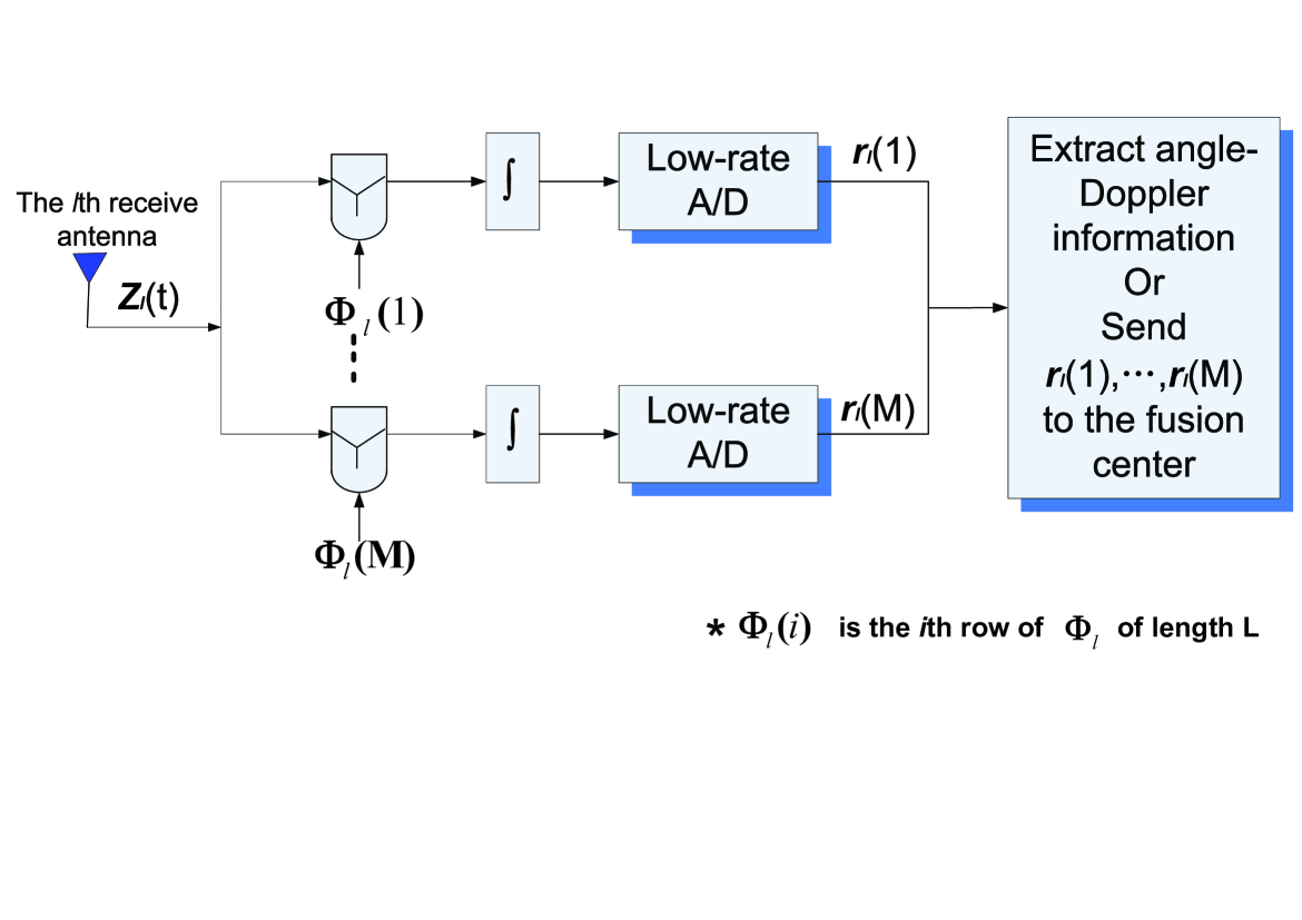
Figure 1: Schematic diagram of the receiver. $\Phi_{l}$ denotes the measurement matrix for the $l$th receive node.

In addition to the computation complexity, the receiver for obtaining the required samples is also more complex. The schematic diagram of the receiver is shown in Fig. 1 (see also [18]).

IV Performance Analysis in the presence of a jammer signal

In [24], Candes and Tao showed that if the basis matrix obeys the UUP and the signal of interest $\bf s$ is sufficiently sparse, then the square estimation error of the Dantzig selector satisfies with very high probability

$$\parallel\hat{\bf s}-{\bf s}\parallel_{\ell_{2}}^{2}\leq C^{2}2logN\times({\sigma}^{2}+\sum_{i}^{N}\min(s^{2}(i),{{\sigma}}^{2}))$$ (26)

where C is a constant, $N$ denotes the length of $\bf s$ and $\sigma^{2}$ is the variance of the noise. It can be easily seen from (26) that an increase in the interference power degrades the performance of the Dantzig selector. Thus, in the presence of a jammer that transmits a waveform uncorrelated with the radar transmit waveforms, the performance of the proposed CS method will deteriorate. Next, we provide analytical expressions for the signal-to-jammer ratio at the receive nodes, and propose a modified measurement matrix to suppress the jammer.

IV-A Analysis of Signal-to-Jammer Ratio

Suppose that each transmitter transmits $N_{p}$ pulses. In the presence of a jammer at location $(d,\theta)$ the signal received at the $l$-th receive antenna can be expressed as

$${\bf r}_{l}=\left[\begin{array}[]{c}{\bf r}_{l1}\\ \vdots\\ {\bf r}_{lN_{p}}\\ \end{array}\right] = \underbrace{\sum_{k=1}^{K}\gamma_{k}e^{j\frac{2\pi}{\lambda}\eta_{l}^{r}(\theta_{k})}\left[\begin{array}[]{c}\mathbf{\Phi}_{l1}e^{j2\pi f_{k}0T}\\ \vdots\\ \mathbf{\Phi}_{lN_{p}}e^{j2\pi f_{k}(N_{p}-1)T}\\ \end{array}\right]{\bf D}(f_{k}){\bf X}{\bf v}(\theta_{k})}_{{\bf r}_{ls}}$$ (40)

$$+\underbrace{e^{-j\frac{2\pi}{\lambda}(d-\eta^{r}_{l}(\theta))}\beta\left[\begin{array}[]{c}\mathbf{\Phi}_{l1}\tilde{{\bf x}}_{1}\\ \vdots\\ \mathbf{\Phi}_{lN_{p}}\tilde{{\bf x}}_{N_{p}}\\ \end{array}\right]}_{{\bf r}_{lj}}+\underbrace{\left[\begin{array}[]{c}\mathbf{\Phi}_{l1}{\bf e}_{l1}\\ \vdots\\ \mathbf{\Phi}_{lN_{p}}{\bf e}_{lN_{p}}\\ \end{array}\right]}_{{\bf r}_{ln}}$$

where $\ \tilde{{\bf x}}_{m}=[\tilde{{x}}_{m}(0T_{s}),\ldots,\tilde{{x}}_{m}((L-1)T_{s})]^{T}$ contains the samples of the signal transmitted by the jammer during the $m$-th pulse, and $\beta$ denotes the square root of the power of the jammer over the duration of one signal pulse.

We assume that for all $m$, $E\{\tilde{x}_{m}^{*}(i)\tilde{x}_{m}(j)\}=1/L$ for $i=j$, and $0$ otherwise. Thus, $E\{\tilde{{\bf x}}^{H}_{m}\tilde{{\bf x}}_{m}\}=1$. Also, we assume that $\tilde{{\bf x}}_{m},\ m=0,\ldots,N_{p}$ are uncorrelated with the main period of the transmitted waveforms. Thus, the effect of the jammer signal is similar to that of additive noise. In the following analysis we assume that the jammer contribution is much stronger than that of additive noise, and therefore we ignore the third term ${\bf r}_{ln}$ on the right hand side of (40). Later, in our simulations we will consider additive noise in addition to a jammer signal.

We assume that all receive nodes use the same random measurement matrix over $N_{p}$ pulses, i.e., $\mathbf{\Phi}_{l}=\mathbf{\Phi}_{l1}=\mathbf{\Phi}_{l2}=\ldots=\mathbf{\Phi}_{lN_{p}}$. Let ${\bf A}_{l}^{k,k^{\prime}}={\bf X}^{H}{\bf D}^{H}(f_{k})\mathbf{\Phi}_{l}^{H}\mathbf{\Phi}_{l}{\bf D}(f_{k^{\prime}}){\bf X}$ and $q^{k,k^{\prime}}_{i,j}$ denote the $(i,j)$-th element of ${\bf A}^{kk^{\prime}}_{l}$. Thus, the average power of the desirable signal conditioned on the transmitted waveform can be represented by

$$P_{s}(l) = E\{{\bf r}^{H}_{ls}{\bf r}_{ls}|{\bf X}\}=E\{\sum_{k,k^{\prime}=1}^{K}\underbrace{\gamma_{k}^{*}\gamma_{k^{\prime}}e^{-j\frac{2\pi}{\lambda}(\eta^{r}_{l}(\theta_{k})-\eta^{r}_{l}(\theta_{k^{\prime}}))}}_{\rho_{l}(k,{k^{\prime}})}\underbrace{(\sum_{m=0}^{N_{p}-1}e^{-j2\pi(f_{k}-f_{k^{\prime}})mT})}_{\mu_{kk^{\prime}}}\underbrace{{\bf v}^{H}(\theta_{k}){\bf A}^{kk^{\prime}}_{l}{\bf v}(\theta_{k^{\prime}})}_{Q_{kk^{\prime}}}\}$$ (41)

$$= N_{p}{E\{\sum_{k=1}^{K}|\beta_{k}|^{2}Q_{kk}\}}+E\{\sum_{k\neq k^{\prime}}\rho_{l}(k,{k^{\prime}})\mu_{kk^{\prime}}Q_{kk^{\prime}}\}$$

where $\rho_{l}(k,{k^{\prime}})$ and $Q_{kk^{\prime}}$ can be further written as

$$\rho_{l}(k,{k^{\prime}}) = e^{j\frac{2\pi}{\lambda}[2(d_{k}(0)-d_{k^{\prime}}(0))-(\eta^{r}_{l}(\theta_{k})-\eta^{r}_{l}(\theta_{k^{\prime}}))}\beta_{k}^{*}\beta_{k^{\prime}}$$ (42)

$$\mathrm{and}\ Q_{kk^{\prime}} = \sum_{i,j}q^{k,k^{\prime}}_{i,j}e^{j\frac{2\pi}{\lambda}(\eta_{j}^{t}(\theta_{k^{\prime}})-\eta_{i}^{t}(\theta_{k}))}\ .$$ (43)

As defined in Section II, the position of the $i$th transmit or receive (TX/RX) node is denoted by $(r_{i}^{t/r},\alpha_{i}^{t/r})$ in polar coordinates. Thus it holds that

$$a_{ji}^{k^{\prime}k}={\eta_{j}^{t/r}(\theta_{k^{\prime}})-\eta_{i}^{t/r}(\theta_{k})}=\left\{\begin{array}[]{rl}2r^{t/r}_{i}\sin(\frac{\theta_{k^{\prime}}-\theta_{k}}{2})\sin(\alpha_{i}-\frac{\theta_{k^{\prime}}+\theta_{k}}{2})&i=j\\ r^{t/r}_{j}\cos(\theta_{k^{\prime}}-\alpha_{j})-r^{t/r}_{i}\cos(\theta_{k}-\alpha_{i})&i\neq j\end{array}\right.$$ (46)

Let $\psi_{0}$ be deterministic. Based on the assumed statistics of $r_{i}$ and $\alpha_{i}$ (see (2)), the distribution of $h=\frac{r_{i}^{t/r}}{r}\sin(\alpha_{i}^{t/r}-\psi_{0})$ is given by ([26])

$$f_{h}(h)=\frac{2}{\pi}\sqrt{1-h^{2}},-1<h<1$$ (47)

and

$$E\left\{e^{j\alpha h}\right\}=2\frac{J_{1}(\alpha)}{\alpha}$$ (48)

where $J_{1}(\cdot)$ is the first-order Bessel function of the first kind. Thus, based on (48) we can obtain

$$E\left\{e^{j\frac{2\pi}{\lambda}{a_{ji}^{k^{\prime}k}}}\right\}=E\left\{e^{j\frac{2\pi r}{\lambda}\frac{a_{ji}^{k^{\prime}k}}{r}}\right\}=\left\{\begin{array}[]{rl}1&i=j\ \text{and}\ k=k^{\prime}\\ \varsigma(4\sin(\frac{\theta_{k^{\prime}}-\theta_{k}}{2}))&i=j\ \text{and}\ k\neq k^{\prime}\\ \varsigma^{2}(2)&i\neq j\end{array}\right.$$ (52)

where $\varsigma(x)=2\frac{J_{1}(x\frac{\pi r}{\lambda})}{x\frac{\pi r}{\lambda}}$.

Therefore, the average power of the desirable signal $P_{s}(l)$ taken over the positions of TX/RX nodes can be found to be

$$P_{s}(l) = N_{p}{E\left\{\sum_{k=1}^{K}|\beta_{k}|^{2}Q_{kk}\right\}}+E\left\{\sum_{k\neq k^{\prime}}\rho_{l}(k,{k^{\prime}})\mu_{kk^{\prime}}Q_{kk^{\prime}}\right\}$$

$$= N_{p}\sum_{k=1}^{K}|\beta_{k}|^{2}E\left\{Q_{kk}\right\}+\sum_{k\neq k^{\prime}}E\left\{\rho_{l}(k,{k^{\prime}})\right\}\mu_{kk^{\prime}}E\left\{Q_{kk^{\prime}}\right\}$$

$$= N_{p}\sum_{k=1}^{K}|\beta_{k}|^{2}\sum_{i,j}q^{k,k}_{i,j}E\{e^{j\frac{2\pi}{\lambda}a_{ji}^{kk}}\}+\sum_{k\neq k^{\prime}}\beta_{k}^{*}\beta_{k^{\prime}}e^{j\frac{4\pi}{\lambda}(d_{k}(0)-d_{k^{\prime}}(0))}E\{e^{j\frac{2\pi}{\lambda}a_{ll}^{k^{\prime}k}}\}\mu_{kk^{\prime}}\sum_{i,j}q^{k,k^{\prime}}_{i,j}E\{e^{j\frac{2\pi}{\lambda}a_{ji}^{k^{\prime}k}}\}$$

$$= N_{p}\sum_{k=1}^{K}|\beta_{k}|^{2}[\sum_{i}q^{k,k}_{i,i}+\sum_{i\neq j}q^{k,k}_{i,j}\varsigma^{2}(2)]$$

$$+\sum_{k\neq k^{\prime}}\beta_{k}^{*}\beta_{k^{\prime}}e^{j\frac{4\pi}{\lambda}(d_{k}(0)-d_{k^{\prime}}(0))}{\varsigma_{kk^{\prime}}}\mu_{kk^{\prime}}[\varsigma_{kk^{\prime}}\sum_{i}q^{k,k^{\prime}}_{i,i}+\sum_{i\neq j}q^{k,k^{\prime}}_{i,j}\varsigma^{2}(2)]$$

where $\varsigma_{kk^{\prime}}=\varsigma(4\sin(\frac{\theta_{k^{\prime}}-\theta_{k}}{2}))$.

For many practical radar systems with wavelength $\lambda$ less than $0.1\mathrm{m}$, (e.g., most military multimode airborne radars), $2\pi r/\lambda$ is a large number if $r>5m$. Since the function $\varsigma(x)$ decreases rapidly as $x$ increases, the terms multiplied by $\varsigma^{2}(2)$ are small enough to be neglected in the above equation. Therefore, (IV-A) can be approximated by

$$P_{s}(l) \approx N_{p}\sum_{k=1}^{K}|\beta_{k}|^{2}\sum_{i}q^{k,k}_{i,i}+\sum_{k\neq k^{\prime}}\beta_{k}^{*}\beta_{k^{\prime}}e^{j\frac{4\pi}{\lambda}(d_{k}(0)-d_{k^{\prime}}(0))}{\varsigma_{kk^{\prime}}}^{2}\mu_{kk^{\prime}}\sum_{i}q^{k,k^{\prime}}_{i,i}\ .$$ (54)

Similarly, the average power of the jammer signal over TR/TX locations is given by

$$P_{j}(l) = E\{{\bf r}_{lj}^{H}{\bf r}_{lj}\}=(e^{-j\frac{2\pi}{\lambda}(d-\eta^{r}_{l}(\theta))}\beta)(e^{-j\frac{2\pi}{\lambda}(d-\eta^{r}_{l}(\theta))}\beta)^{*}\sum_{m=1}^{N_{p}}\tilde{{\bf x}}_{m}^{H}{\mathbf{\Phi}}^{H}_{l}{\mathbf{\Phi}}_{l}\tilde{{\bf x}}_{m}$$ (55)

$$= |\beta|^{2}\sum_{m=1}^{N_{p}}\tilde{{\bf x}}_{m}^{H}{\mathbf{\Phi}}^{H}_{l}{\mathbf{\Phi}}_{l}\tilde{{\bf x}}_{m}.$$

The SJR given the node locations is the ratio of the power of the signal to the power of the jammer. Since the denominator does not depend on node locations, the average SJR equals SJR$=P_{s}(l)/P_{j}(l)$.

Some insight into the above obtained expression will be given in the following for some special cases.

IV-B SJR based on a modified measurement matrix

Since the jammer signal is uncorrelated with the transmitted signal, the SJR can be improved by correlating the jammer signal with the transmitted signal. Therefore, we propose a measurement matrix of the form

$$\tilde{\mathbf{\Phi}}_{l}=\mathbf{\Phi}^{\prime}_{l}{\bf X}^{H}\ (M\times L)$$ (56)

where $\mathbf{\Phi}^{\prime}_{l}$ is an $M\times M_{t}$ Gaussian random matrix. Note that $\tilde{\mathbf{\Phi}}_{l}$ is also Gaussian. As stated in [12], a random measurement matrix with i.i.d. entries, e.g., Gaussian or $\pm 1$ random variables, is nearly incoherent with any fixed basis matrix. Therefore, the proposed measurement matrix exhibits low coherence with $\Psi_{l}$, thus guaranteeing a stable solution to (23). Based on (56), the average power of the desirable signal $P_{s}(l)$ is given by (IV-A), except that $Q_{kk^{\prime}}$ is based on ${\bf A}_{l}^{k,k^{\prime}}={\bf X}^{H}{\bf D}^{H}(f_{k}){\bf X}(\mathbf{\Phi}^{\prime}_{l})^{H}\mathbf{\Phi}^{\prime}_{l}{\bf X}^{H}{\bf D}(f_{k^{\prime}}){\bf X}$. The average power of the jammer signal is given by (55) where ${\bf\Phi}_{l}$ is replaced by $\tilde{{\bf\Phi}}_{l}$.

Let us assume that the $M_{T}$ transmit nodes emit periodic pulses containing independent quadrature phase shift keying (QPSK) symbols, and that ${\bf X}^{H}{\bf X}={\bf I}_{M_{t}}$. Also, we assume that ${\mathbf{\Phi}}_{l}{\mathbf{\Phi}}_{l}^{H}={\mathbf{\Phi}}^{\prime}_{l}({\mathbf{\Phi}}^{\prime}_{l})^{H}={\bf I}_{M}$.

Let $\tilde{x}_{i}(n)$ be expressed as $\vartheta_{in}/\sqrt{L}$, where $\vartheta_{in}$ is a random variable with mean zero and variance one. Then the average power of the jammer signal $P_{j}(l)$ can be rewritten as follows:

$$P_{j}(l) = |\beta|^{2}\sum_{m=1}^{N_{p}}\tilde{{\bf x}}_{m}^{H}{\mathbf{\Phi}}^{H}_{l}{\mathbf{\Phi}}_{l}\tilde{{\bf x}}_{m}$$ (57)

$$= |\beta|^{2}\sum_{m=1}^{N_{p}}\sum_{i=j=0}^{L-1}\tilde{{x}}^{*}_{m}(i)\tilde{{x}}_{m}(i)c_{ii}+|\beta|^{2}\sum_{m=1}^{N_{p}}\sum_{i\neq j=0}^{L-1}\tilde{{x}}^{*}_{m}(i)\tilde{{x}}_{m}(j)c_{ij}$$

$$= \frac{1}{L}|\beta|^{2}\sum_{m=1}^{N_{p}}\sum_{i=0}^{L-1}\vartheta^{*}_{mi}\vartheta_{mi}c_{ii}+\frac{1}{L}|\beta|^{2}\sum_{m=1}^{N_{p}}\sum_{i\neq j=0}^{L-1}\vartheta^{*}_{mi}\vartheta_{mj}c_{ij}$$

where $c_{ij}$ is the $(i,j)$-th entry of ${\mathbf{\Phi}}^{H}_{l}{\mathbf{\Phi}}_{l}$. Since the entries of ${\mathbf{\Phi}}_{l}$ are i.i.d Gaussian variables with zero means and variances $\frac{1}{L}$, $c_{ii},i=1,\ldots,L$ are i.i.d chi-square random variables with means $\frac{M}{L}$ and variances $\frac{2M}{L}$; $c_{ij},i\neq j$ are of mean zero and variance $M/L^{2}$. Let us express $c_{ij},i\neq j$ as $\varrho_{ij}\sqrt{M}/L$, where $\varrho_{ij}$ has zero mean and unit variance. It holds that

$$P_{j}(l) = |\beta|^{2}\sum_{m=1}^{N_{p}}E\{\vartheta^{*}_{mi}\vartheta_{mi}c_{ii}\}+\frac{\sqrt{M}}{L^{2}}|\beta|^{2}\sum_{m=1}^{N_{p}}\sum_{i\neq j=0}^{L-1}\vartheta^{*}_{mi}\vartheta_{mj}\varrho_{ij}$$ (58)

$$= |\beta|^{2}N_{p}\frac{M}{L}+\frac{|\beta|^{2}\sqrt{M}(L-1)}{L}\sum_{m=1}^{N_{p}}\frac{1}{L(L-1)}\sum_{i\neq j=0}^{L-1}\vartheta^{*}_{mi}\vartheta_{mj}\varrho_{ij}$$

$$= N_{p}|\beta|^{2}\frac{M}{L}+\frac{|\beta|^{2}\sqrt{M}(L-1)}{L}\sum_{m=1}^{N_{p}}E\{\vartheta^{*}_{i,m}\vartheta_{j,m}\varrho_{ij}\}$$

$$\approx N_{p}|\beta|^{2}\frac{M}{L}$$

where we have used the fact that for large $L$,

$$\frac{1}{L}\sum_{i=0}^{L-1}\vartheta^{*}_{mi}\vartheta_{mi}c_{ii} \rightarrow E\{\vartheta^{*}_{mi}\vartheta_{mi}c_{ii}\}=\frac{M}{L}$$ (59)

$$\mathrm{and}\ \frac{1}{L(L-1)}\sum_{i\neq j=0}^{L-1}\vartheta^{*}_{mi}\vartheta_{mj}\varrho_{ij} \rightarrow E\{\vartheta^{*}_{mi}\vartheta_{mj}\varrho_{ij}\}=0\ .$$ (60)

Using the measurement matrix $\tilde{\mathbf{\Phi}}_{l}$ in (56) will not affect the average $P_{j}(l)$ over the jammer signal due to the fact that $\sum_{i}c_{ii}=\mathrm{Tr}\{{\bf X}(\mathbf{\Phi}^{\prime}_{l})^{H}\mathbf{\Phi}^{\prime}_{l}{\bf X}^{H}\}=\mathrm{Tr}\{{\bf X}^{H}{\bf X}(\mathbf{\Phi}^{\prime}_{l})^{H}\mathbf{\Phi}^{\prime}_{l}\}=\mathrm{Tr}\{\mathbf{\Phi}^{\prime}_{l}(\mathbf{\Phi}^{\prime}_{l})^{H}\}=\mathrm{Tr}\{{\bf I}_{M}\}=M$.

In the following, we will look into the SJR improvement using $\tilde{\mathbf{\Phi}}_{l}$ as opposed to ${\mathbf{\Phi}}_{l}$, for two different cases, i.e., stationary targets and moving targets.

IV-B1 Stationary Targets

First, let us consider the SJR using the random measurement matrix $\mathbf{\Phi}_{l}$.

When the targets are stationary, the Doppler shift is zero and so ${\bf A}_{l}^{k,k^{\prime}}={\bf A}_{l}={\bf X}^{H}\mathbf{\Phi}_{l}^{H}\mathbf{\Phi}_{l}{\bf X}$. Therefore, the average power of the desired signal can be approximated as

$$P_{s}(l) \approx N_{p}\sum_{k=1}^{K}|\beta_{k}|^{2}\sum_{i}q_{i,i}+N_{p}\sum_{k\neq k^{\prime}}\beta_{k}^{*}\beta_{k^{\prime}}e^{j\frac{4\pi}{\lambda}(d_{k}(0)-d_{k^{\prime}}(0))}\varsigma_{kk^{\prime}}^{2}\sum_{i}q_{i,i}$$ (61)

where $q_{i,j}$ is the $(i,j)$-th entry of ${\bf A}_{l}$.

Letting ${\bf x}_{i}$ denote the $i$-th column of ${\bf X}$, $\sum_{i}q_{i,i}$ can be expressed as

$$\sum_{i}q_{i,i} = \mathrm{Tr}\{{\bf A}_{l}\}=\sum_{i=1}^{M_{t}}{\bf x}^{H}_{i}\mathbf{\Phi}_{l}^{H}\mathbf{\Phi}_{l}{\bf x}_{i}=\sum_{i=1}^{M_{t}}\sum_{m,n=1}^{L}x^{*}_{i}(m)c_{mn}x_{i}(n)$$ (62)

$$= \sum_{i=1}^{M_{t}}\sum_{m=1}^{L}x^{*}_{i}(m)x_{i}(m)c_{mm}+\sum_{i=1}^{M_{t}}\sum_{m\neq n}^{L}x^{*}_{i}(m)x_{i}(n)c_{mn}.$$

The entries of ${\bf X}$ have zero means and mutually independent; therefore, for sufficiently long $L$ and $M_{t}$ it holds that

$$\sum_{i}q_{i,i} = \frac{M_{t}}{L}\sum_{m=1}^{L}c_{mm}=\frac{MM_{t}}{L}.$$ (63)

Based on (63), a concise form of $P_{s}(l)$ is given by

$$P_{s}(l) \approx \frac{N_{p}MM_{t}\sum_{k=1}^{K}|\beta_{k}|^{2}}{L}+\frac{N_{p}MM_{t}}{L}\varphi$$ (64)

where $\varphi=\sum_{k,k^{\prime},k\neq k^{\prime}}\beta_{k}^{*}\beta_{k^{\prime}}e^{j\frac{4\pi}{\lambda}(d_{k}(0)-d_{k^{\prime}}(0))}\varsigma_{kk^{\prime}}^{2}$.

Thus, the SJR corresponding to the random measurement matrix $\mathbf{\Phi}_{l}$ is

$$SJR_{l}=\frac{P_{s}(l)}{P_{j}(l)}\approx\frac{M_{t}(\sum_{k=1}^{K}|\beta_{k}|^{2}+\varphi)}{|\beta|^{2}}\ .$$ (65)

When using the measurement matrix $\tilde{\mathbf{\Phi}}_{l}=\mathbf{\Phi}^{\prime}_{l}{\bf X}^{H}$, the quantity corresponding to ${\mathbf{A}}_{l}^{k,k^{\prime}}$ is

$$\tilde{{\bf A}}_{l}^{k,k^{\prime}}=\tilde{{\bf A}}_{l}={\bf X}^{H}{\bf X}(\mathbf{\Phi}^{\prime}_{l})^{H}\mathbf{\Phi}^{\prime}_{l}{\bf X}^{H}{\bf X}=(\mathbf{\Phi}^{\prime}_{l})^{H}\mathbf{\Phi}^{\prime}_{l}\ .$$ (66)

It holds that $\sum_{i}q_{i,i}=\mathrm{Tr}\{(\mathbf{\Phi}^{\prime}_{l})^{H}\mathbf{\Phi}^{\prime}_{l}\}=\mathrm{Tr}\{\mathbf{\Phi}^{\prime}_{l}(\mathbf{\Phi}^{\prime}_{l})^{H}\}=M$. Similarly, the average power of the desired signal can be approximated as

$$P_{s}(l) \approx N_{p}M(\sum_{k=1}^{K}|\beta_{k}|^{2}+\varphi).$$ (67)

Therefore, the SJR corresponding to the random measurement matrix $\tilde{\mathbf{\Phi}}_{l}$ is

$$SJR_{l}=\frac{P_{s}(l)}{P_{j}(l)}\approx\frac{L(\sum_{k=1}^{K}|\beta_{k}|^{2}+\varphi)}{|\beta|^{2}}\ .$$ (68)

From (65) and (68), it can be seen that the use of $\tilde{\mathbf{\Phi}}_{l}$ instead of ${\mathbf{\Phi}}_{l}$ can improve SJR by a factor of $L/M_{t}$ when $L\gg M_{t}$. The SJR can be improved by an increase in $L$. However, increasing $L$ will require a higher sampling rate when the pulse duration is fixed. It is interesting to note that the SJR of (68) does not depend on the the number of measurements, $M$.

IV-B2 Slowly Moving Targets

For simplicity, we consider only the scenarios in which $f_{k}T<<1$.

Based on the measurement matrix $\mathbf{\Phi}_{l}$, and considering the Doppler shift, we have ${\bf A}_{l}^{k,k^{\prime}}={\bf X}^{H}{\bf D}^{H}(f_{k})\mathbf{\Phi}_{l}^{H}\mathbf{\Phi}_{l}{\bf D}(f_{k^{\prime}}){\bf X}$. When the normalized Doppler frequency $f_{k}T_{s}\leq 1$, we have

$$\sum_{i}q^{k,k^{\prime}}_{i,i}=\mathrm{Tr}\{{\bf A}_{l}^{k,k^{\prime}}\}=\mathrm{Tr}\{{\bf X}^{H}{\bf D}^{H}(f_{k})\mathbf{\Phi}_{l}^{H}\mathbf{\Phi}_{l}{\bf D}(f_{k^{\prime}}){\bf X}\}\approx\frac{MM_{t}}{L}.$$ (69)

Thus, $P_{s}(l)$ for the moving targets with $f_{s}T<<1$ is approximately the same as that of stationary targets.

Let us now consider the measurement matrix $\tilde{\mathbf{\Phi}}_{l}$. Let $c_{ij}^{k}$ denote the $(i,j)$-th entry of ${\bf X}^{H}{\bf D}^{H}(f_{k}){\bf X}$ and note that $c_{ij}^{k}$ is given by $c_{ij}^{k}=\sum_{n=0}^{L-1}x_{i}^{*}(n)x_{j}(n)*e^{j2\pi f_{k}nT_{s}}$. In scenarios in which $f_{k}T_{s}<<1$ and $L$ is relatively large, the following approximations are readily derived:

$$c_{ij}^{k}\left\{\begin{array}[]{cccc}&=&\frac{1}{L}\frac{1-e^{j2\pi f_{k}LT_{s}}}{1-e^{j2\pi f_{k}T_{s}}}&i=j\\ &\approx&0&i\neq j\end{array}\right.\ .$$ (72)

Since the off-diagonal elements are small compared with the diagonal elements, they can be ignored.

Then, we obtain the following approximation

$${\bf A}_{l}^{k,k}={\bf X}^{H}{\bf D}^{H}(f_{k}){\bf X}(\mathbf{\Phi}^{\prime}_{l})^{H}\mathbf{\Phi}^{\prime}_{l}{\bf X}^{H}{\bf D}(f_{k}){\bf X}\approx(\mathbf{\Phi}^{\prime}_{l})^{H}\mathbf{\Phi}^{\prime}_{l}.$$ (73)

Therefore, the SJR of moving targets with $f_{s}T<<1$ is approximately equal to that of stationary targets for both random measurement matrices.

V Simulation Results

The goal of this section is to demonstrate the ability of the proposed MIMO radar approach, denoted in the figures as CS, to pick up targets in the presence of noise and/or a jammer, and also show the effect on the various parameters involved. In each case the performance is compared against other methods that have been proposed in the context of MIMO radar (here referred to as “conventional”) in order to quantify weaknesses and advantages. For the case of stationary targets, the conventional methods tested here are the methods of Capon, APES, GLRT [2] and MUSIC [27], while for moving targets, comparison to the matched filter method [21] is conducted.

In our simulations we consider a MIMO radar system with the transmit/receive antennas uniformly distributed on a disk of radius $10$m. The carrier frequency is $f=5GHz$ and the sampling rate $f_{s}=\frac{1}{T_{s}}=20MHz$. The pulse repetition interval is $T=1/4000s$. Each transmit node uses uncorrelated QPSK waveforms. The received signal is corrupted by zero mean Gaussian noise. We also consider a jammer that transmits waveforms uncorrelated to the signal waveforms. For simulation purposes we take the jamming waveforms to be white Gaussian [28]. The SNR is defined as the ratio of power of transmit waveform to that of thermal noise at a receive node.

V-A Stationary Targets

The presence of a target can be seen in the plot of the magnitude of $\hat{{\bf s}}$ obtained by (23). We will refer to this vector as target information vector. The location and magnitude of a peak in that plot provides target location and RCS magnitude, respectively. The proposed approach results in a clean plot away from the target locations, and well distinguished peaks corresponding to the targets. This is a desirable behavior for target detection, as it would result in small probability of false alarm. To demonstrate the appearance of the graph we define the peak-to-ripple ratio (PRR) metric as follows. For the $k$-th target, PRR_k is the ratio of the square amplitude of the DOA estimate at the target azimuth angle to the sum of the square amplitude of DOA estimates at other angles except at the jammer location, i.e., $PRR_{k}=\frac{|s_{k}|^{2}}{{\bf s}^{H}{\bf s}-\sum_{i=1}^{K}|s_{k}|^{2}-|s_{j}|^{2}}$, where ${\bf s}$ is the defined in (18), $s_{k}$ and $s_{j}$ denote the elements of $\bf s$ corresponding to the location of the $k$-th target and the jammer, respectively. A clean plot would yield a high PPR, while a plot with a lot of ripples would yield a low PRR.

A metric that shows the degree to which a jammer is suppressed, namely the peak-to-jammer ratio (PJR), is also used here. PJR is defined as the ratio of the average square amplitude of the DOA estimates at the target angles to the square amplitude of DOA estimates at the jammer, i.e., $PJR=\frac{\frac{1}{K}\sum_{i=1}^{K}|s_{k}|^{2}}{|s_{j}|^{2}}$. Unlike PRR, PJR is averaged over all targets. In this way, the jammer is considered to be suppressed only if the peak amplitude at the jammer location is much smaller than the peak amplitude at any target location.

The results that we show represent $1,000$ Monte Carlo simulations over independent waveforms and noise realizations. To better show the statistical behavior of the methods we plot the cumulative density function (CDF) of PPR and PJR, i.e., $Probability(PPR<x)$ and $Probability(PJR<x)$, where $PPR$ is the union of $PRR_{k},k=1,\ldots,\ K$.

V-A1 Targets falling on the grid

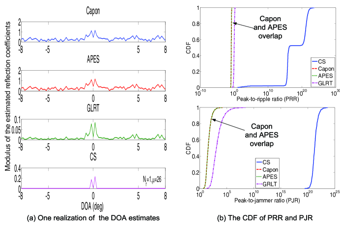
Figure 2: One realization of the DOA estimates (left column) and CDF of PPR and PJR (right column). $N_{r}=1$, $M_{t}=M=30$, $\beta^{2}=400$, SNR$=0$ dB and $\mu=26$.

We consider the following scenario. Two targets are located at angles $\theta_{1}=0.2\textordmasculine$ and $\theta_{2}=-0.2\textordmasculine$. The corresponding reflection coefficients are $\beta_{1}=\beta_{2}=1$. A jammer is located at angle $7\textordmasculine$ and transmits an unknown zero-mean Gaussian random waveform with variance $\beta^{2}=400$. Additive white Gaussian noise is added at the receive nodes. The ratio of the power of transmitted waveforms at each transmit node to the variance of the additive Gaussian noise is set to $0$ dB. The number of transmit antennas is fixed at $M_{t}=30$. For the purpose of reducing computation time, the angle space is taken to be $[-8\textordmasculine,8\textordmasculine]$, and is sampled with increments of $0.2\textordmasculine$ from $-8\textordmasculine$ to $8\textordmasculine$, i.e., ${\bf a}=[-8\textordmasculine,-7.8\textordmasculine,\ldots,7.8\textordmasculine,8\textordmasculine]$. The received signal in a single pulse is sampled, and $M=30$ random measurements of one pulse are used to feed the Dantzig selector. Since the MUSIC method requires the number of receive antennas to be greater than the number of targets, when only one receive antenna is used we compare the proposed CS method with only the Capon, APES and GLRT methods. The comparison methods are using $L=512$ samples to obtain their estimates, while the proposed approach uses $M=30$ samples. The result of one realization for the case of one receive node is shown in Fig. 2. One can observe the cleaner appearance of the graph corresponding to the proposed approach, where the two targets appear correctly except with a small error in the magnitude of the target RCS. The CDF of the corresponding PRR and PJR are also shown in the same figure. One can clearly see that with one receive antenna the comparison methods yield PRR close to $1$, which is indicative of severe ripples.

In general, an increase in the number of transmit snapshots $L$ leads to improved PRR and PJR for all methods. In the following results we fix $L$ to $512$. For the comparison methods, $L$ represents that number of samples needed to obtain target information. For CS, the number of samples used to extract target information is $M$.

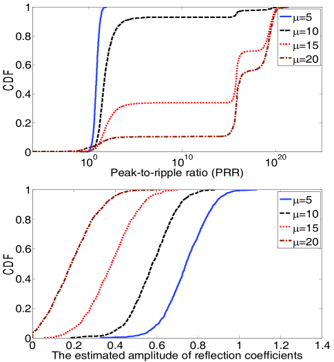
Figure 3: CDF of PRR (top) and amplitude estimate of RCS (bottom).

For the scenario of Fig. 2, the effect of the threshold $\mu$ is evaluated in terms of the empirical CDF of the PRR and the amplitude estimate of RCS, and the results are shown in Fig. 3. One can can see that the increase in $\mu$ can lead to fewer ripples but at the same time it degrades the amplitude estimate of RCS. In the following, the values of $\mu$ used in each case will be shown on the figures.

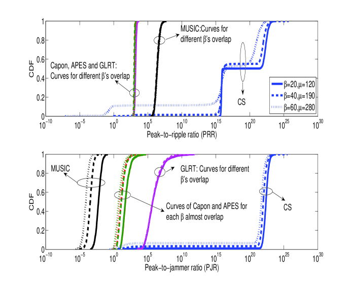
Figure 4: CDF of PRR and SJR for $\beta=20,40,60$ with $N_{r}=10,M_{t}=M=30$ and SNR$=0$ dB. The corresponding thresholds are $\mu=120,190$ and $280$.

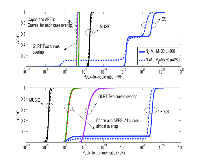
Figure 5: CDF of PRR and SJR for $\beta^{2}=3600$ and SNR=$0$ dB. Two cases are shown, $(N_{r}=10,M_{t}=30,M=30)$ and $(N_{r}=30,M_{t}=30,M=30)$. The corresponding thresholds are $\mu=280$ and $800$.

For the same target and jammer configuration as above, we now examine the effect of different levels of jammer strength. We consider the scenario where $N_{r}=10$ receive nodes participate in the estimation. For the case of CS, each node sends to the fusion center $M=30$ received samples, while for the comparison methods, each node sends to the fusion center $L=512$ received samples. In Fig. 4 we show the CDF of PPR and PJR corresponding to jammer variance $\beta^{2}=400,1600$ and $3600$ and SNR equal to $0$ dB. One can see that for CS, the probability of low PRR and PJR increases when the jammer becomes stronger. In particular, there is some non-zero probability that the PRR will be close to $10^{-7}$. Such cases are rare and occur when one of the two targets is missed. The increase in the threshold $\mu$ can improve the DOA estimates at the target locations and reduce the probability of missing one of the targets. The cost, however, would be an increase in ripples. The performance of the proposed approach can be improved, i.e., the rare low PPR values can be completely avoided by increasing $N_{r}$, or $M$. This is demonstrated in Fig. 5, where the strong jammer case of Fig. 4 is considered, i.e., $\beta^{2}=3600$, and $N_{r}$ is increased to $30$. We should note here that it does not help to increase $M$ beyond $M_{t}$ as the maximal rank of $\Phi^{\prime}_{l}$ is $M_{t}$.

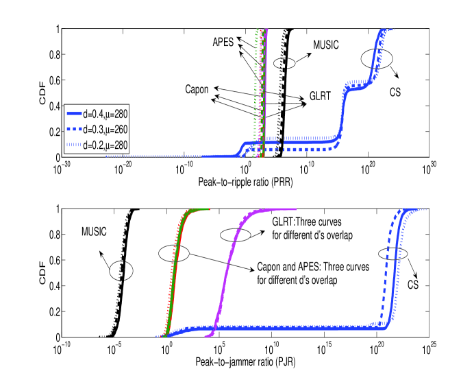
Figure 6: DOA estimates of two targets with spacing $d=0.4\textordmasculine,0.3\textordmasculine$ and $0.2\textordmasculine$. $N_{r}=10,M_{t}=M=30$, SNR=$0$ dB and $\beta^{2}=3600$. The corresponding thresholds are $\mu=280,260$ and $280$.

Next, we consider the same scenario as above but let the two targets be at variable distance $d$ in the angle domain. Figure 6 demonstrates performances for the cases $d=0.2\textordmasculine,0.3\textordmasculine,0.4\textordmasculine$ in the presence of a strong jammer with variance $\beta^{2}=3600$. The SNR is $0$ dB, $N_{r}=10$ and $M=30$. One can see that the comparison methods produce good level PRR. Regarding the PJR, as expected, MUSIC fails, Capon and APES results is PRR$\approx 1$ most of the time, while GLRT performs well all the time. The proposed CS approach performs well with a few exceptions in which a PRR or PJR less than $1$ is obtained with very small probability. Again, the CS method performance can be improved by increasing $N_{r}$ and/or $M$.

Based on the above results, the performance of the proposed approach for the jammer dominated scenario can be made at least comparable to that of the conventional methods while using about $5.8\%\ (=30/512)$ of the number of samples required by the conventional methods.

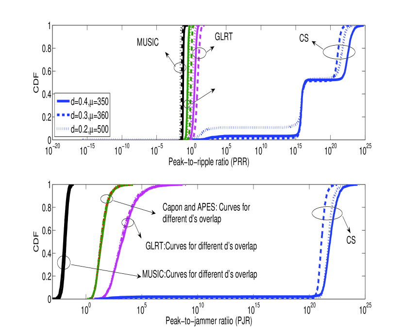
Figure 8: CDF of PRR and PJR for two targets with the spacing $d=0.4\textordmasculine,0.3\textordmasculine$ and $0.2\textordmasculine$. $N_{r}=20,M_{t}=M=30$, SNR=$-40$ dB and $\beta=20$.

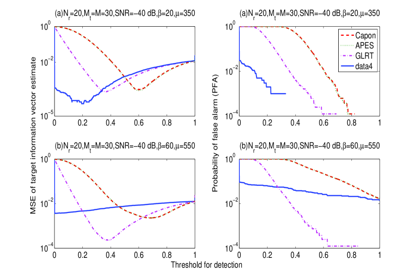
Figure 9: MSE of target information vector and probability of false alarm (PFA) for two targets with spacing $d=0.4\textordmasculine$ for $N_{r}=20,M_{t}=M=30$ and SNR$=-40$ dB.

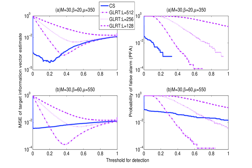
Figure 10: MSE of target information vector and probability of false alarm (PFA) for two targets with spacing $d=0.4\textordmasculine$ for $N_{r}=20,M_{t}=M=30$ and SNR$=-40$ dB. The number of transmit waveforms and receive samples per pulse for CS is 512 and 30, respectively.

Next, we study a thermal noise dominated case, i.e., SNR=$-40$dB. Figure 7 shows PRR and PJR performance for different values of jammer variance, i.e., $\beta^{2}=400,1600$ and $3600$. In all cases it was taken $N_{r}=10$, $M_{t}=M=30$ and the targets were separated by $d=0.4\textordmasculine$. CS yields good performance even in the presence of both a strong jammer and thermal noise. The PRR performance of other methods appear to deteriorate at this noise level. The performances for targets with spacing $d=0.2\textordmasculine,0.3\textordmasculine$ and $0.4\textordmasculine$ are given in Fig. 8 for $N_{r}=20$, $M_{t}=M=30$ and $\beta^{2}=400$. Like in the case of a strong jammer, the decrease in the spacing $d$ does not affect the performance significantly. In this thermal noise dominated case, CS appears to perform very well in terms of PRR, and PJR, while the comparison methods appear to be very noisy. To further examine this case, we consider two additional performance measures, i.e., mean squared error (MSE) and probability of false alarm (PFA), which are computed based on the obtained estimate $\hat{\bf s}$ as follows. A new vector, $\hat{\bf s}^{t}$ is formed; if $\hat{s}_{i}$ is greater than some threshold then $\hat{s}^{t}_{i}=1$, otherwise, $\hat{s}^{t}_{i}=0$. The MSE is calculated as $MSE=\|\hat{{\bf s}}_{t}-{\bf s}_{t}\|^{2}_{2}/N$, where ${\bf s}_{t}$ is an $N\times 1$ vector which contains zeros everywhere except at angles corresponding to target locations, where it is $1$. The PFA measures the probability of $1$ occurring in $\hat{{\bf s}}$ at non-target locations. Figure 9 shows the MSE based on $8,000$ Monte Carlo simulations. Note that the performance of MUSIC is not shown here since MUSIC always yields a peak at the jammer location. One can see that the simple thresholding described above helps the comparison methods, and if the threshold is picked appropriately all methods can produce a low angle MSE and PFA. However, the MSE corresponding to the CS method is less sensitive to the particular threshold than other methods. For the milder jammer case ($\beta=20$), the CS approach exhibits slightly better “best MSE performance” than the comparison methods, while in the stronger jammer case ($\beta=60$) GLRT outperforms CS for most thresholds. For the strong jammer case, the MSE and PFA of CS are compared to those of GLRT for different number of samples, $L$ in Fig. 10. One can see that for the strong jammer case ($\beta=60$) CS performs comparably to GLRT with $L=256$. Thus, in the strong jammer case, CS still achieves good performance with fewer samples than GLRT, except that the savings in terms of number of samples is smaller. For CS, the trend of an increasing MSE as the threshold increases can be explained by the fact that one of the two targets can be missed as the threshold increases. GLRT relies on the Gaussian assumption for the noise and jammer signals, which is totally valid in our simulations. Thus, unlike the other methods, GLRT can suppress the jammer completely. We should note that the specific values of MSE and PFA depend on the kind of thresholding performed. For example, applying thresholding on a nonlinear transformation of the estimated vector can give different MSE and PFA, and the best results for each method are not necessarily obtained based on the same non-linear transformation. Determining the best thresholding method is outside the scope of this paper.

V-A2 Targets falling off the grid points

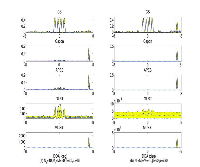
Figure 11: Modulus of DOA estimates for four targets that do not fall on grid points. The dotted line is the mean of DOA estimates. The yellow region is the area bounded by the curves mean $\pm$ std.

In this section, we consider scenarios in which targets do not fall on the grid points. This is a case of practical interest, as the target locations are unknown, thus the best grid in not known in advance. We first select the proper step to discretize the angle space following the procedures described in Section III-B. The angle space is sampled by increments of $0.2\textordmasculine$ from $-8\textordmasculine$ to $8\textordmasculine$, i.e., ${\bf a}=[-8\textordmasculine,-7.8\textordmasculine,\ldots,7.8\textordmasculine,8\textordmasculine]$. Assume that four targets of interest are located at $\theta_{k}=\{-1.1\textordmasculine,-0.3\textordmasculine,0.3\textordmasculine,1.1\textordmasculine\}$. Their reflection coefficients are $\{\beta_{k}=1,k=1,2,3,4\}$. A jammer is still located at $7\textordmasculine$. Since the targets are located between the grid points, we cannot plot PRR and PJR as in the case of targets onto the grid points. Therefore, we show the mean plus and minus one standard deviation (std) for the amplitude of DOA estimate at each grid point. The results are shown in Fig. 11. The power of the jammer was $400$ (left column of Fig. 11) and $3600$ (right column). Based on Fig. 11, it can be seen that with the proper grid points, the proposed method can capture well the targets that do not fall on grid points. The next best method is the GLRT which captures the targets but exhibits high variance as indicated by the shaded region around the mean.

V-B Moving Targets

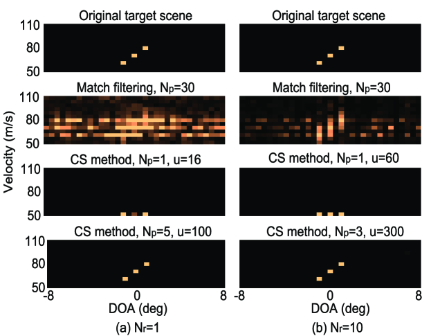
Figure 12: Angle-Doppler estimates for three targets on the grid points. The three targets are located at {-1º, 0º, 1º}. $M_{t}=M=30$, SNR$=0$ dB and $\beta^{2}=400$.

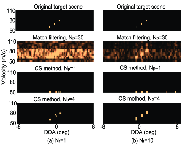
Figure 13: Angle-Doppler estimates for three targets that do not fall on the grid points. The three targets are located at {-1.1º, 0.1º, 1.1º}. $M_{t}=M=30$, $\beta^{2}=400$ and SNR$=0$ dB.

We continue to consider orthogonal QPSK waveforms and a jammer located at $7\textordmasculine$ with the power $400$. The SNR is still set to be $0$ dB and each receive node collects $M=30$ measurements. Figures 12 and 13 show the target scene of the proposed CS method and the matched filter approach [21] for targets on the grid points and off the grid points, respectively. The matched filter correlates the receive signal with the transmit signal distorted by different Doppler shifts and steering vectors.

V-B1 Targets falling onto the grid points

We assume the presence of three targets located at $\{\theta_{k}=-1\textordmasculine,\ 0\textordmasculine,\ 1\textordmasculine\}$ that are moving at the speed of $\{v_{k}=60m/s,\ 70m/s,\ 80m/s\}$, respectively. We sample the angle-Doppler space by the increment $(0.5\textordmasculine,5m)$ as

$${\bf a}=[(-8\textordmasculine,50m/s),(-7.5\textordmasculine,50m/s),\ldots,(8\textordmasculine,50m/s),(-8\textordmasculine,55m/s)\ldots,(8\textordmasculine,55m/s),\ldots,\ldots,(8\textordmasculine,110m/s)]$$ (74)

Figure 12 shows the target scene for one realization corresponding to $N_{1}=1$ receive nodes (left column of the figure), and also $N_{r}=10$ (right column of the figure). We can see that the performance of the match filtering method is inferior to that of the CS approach even when using the data of $30$ pulses. The proposed CS approach can yield the desired performances even with a single receive node and as low as $5$ pulses. Comparing the left column and right column of Fig. 12, one can see the effect of the number of receive antennas $N_{r}$. The increase in $N_{r}$ can reduce the number of pulses required to produce good performance.

V-B2 Targets falling off the grid points

In this section, we consider the scenarios in which targets that do not fall on grid points. From simulations (the corresponding figure is not given here because of space limitations), we found that the column correlation is more sensitive to the angle step than the speed step, since $fT_{s}<<1$. This indicates that in the initial estimation, the grid points should be closely spaced in the angle axis and relatively sparser in the speed axis. Then the resolution of target detection can be improved by taking denser samples of the angle-Doppler space around the initial angle-Doppler estimate.

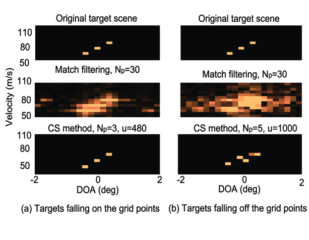
Figure 14: Angle-Doppler estimates for three targets on and off grid points. $N_{r}=10$, $M_{t}=M=30$, SNR$=0$ dB, $\beta^{2}=400$ and $d=0.4\textordmasculine$.

Like the scenarios with the stationary targets, the angle dimension is sampled by increments of $0.2\textordmasculine$ and the step of the speed dimension is set to $5m/s$. Three targets are moving at the speed of $\{v_{k}=62.5m/s,\ 72.5m/s,\ 82.5m/s\}$ in the direction of $\{\theta_{k}=-1.1\textordmasculine,\ 0.1\textordmasculine,\ 1.1\textordmasculine\}$. Fig.13 demonstrates that the proposed method can capture the targets which fall out of the grid points in both angle and speed dimensions and it can outperform the conventional matched filter method. Moreover, we can see that the increase in $N_{p}$ or $N_{r}$ will not necessarily improve performance for the targets between grid points. This is because an increase in the dimension of the basis vectors will decrease the correlation of columns in the basis matrix, which contradicts the requirement for capturing the targets out of the grid points III-B. The performance in the case of closer spaced targets, i.e., $d=0.4\textordmasculine$ is shown in Fig. 14.

VI Conclusions

We have proposed a MIMO radar system that can be implemented by a small-sized wireless network. Network nodes serve as transmitters or receivers. Transmit nodes transmit uncorrelated waveforms. Each receive node applies compressive sampling to the received signal to obtain a small number of samples, which the node subsequently forwards to a fusion center. Assuming that the targets are sparsely located in the angle-Doppler space, the fusion center formulates an $\ell_{1}$-optimization problem, the solution of which yields target angle and Doppler information. For the stationary case, the performance of the proposed approach was compared to that of conventional approaches that have been proposed in the context of MIMO radar. The comparison scenario assumed that each receive node forwards the received signal to a fusion center, where Capon, APES, GLRT or MUSIC is implemented to obtain target information. The proposed approach can extract target information based on a small number of measurements from one of more receive nodes. In particular, for a mild jammer, the proposed method has been shown to be at least as good as the Capon, APES, GLRT and MUSIC techniques while using a significantly smaller number of samples. In the case of strong thermal noise and strong jammer, the proposed method performs slightly worse than the GLRT method. In that case, its performance is still acceptable, especially if one takes into account the fact that it uses significantly fewer samples than GLRT. For the case of moving targets, the proposed approach was compared to conventional matched filtering, and was shown to perform better in both single and multiple receive nodes cases. An important feature of the proposed approach is energy savings. If the fusion center implemented the proposed CS approach, it would require nodes to forward $M$ samples each, as opposed to $L$ samples that would be needed if the fusion center implemented the conventional methods. In order to meet a certain performance, $M$ is typically significantly smaller than $L$, i.e., fewer samples would be needed for the CS implementation as compared to the implementation of conventional methods. This translates to energy savings during the transmission of the samples from the receive nodes to the fusion center. The obtained savings would be significant in prolonging the life of the wireless network. Future work includes extension to extracting range information, and also studying scenarios of widely separated antennas and wideband radar signals. The proposed approach assumes that nodes are synchronized and the fusion center has perfect node location information. The effects of localization and synchronization errors and ways to mitigate them need to be further studied.

Acknowledgment

The authors would like to thank Dr. Rabinder Madan of the Office of Naval Research for sharing his ideas on the use of compressive sampling in the context of MIMO radar, and also the Associate Editor and the anonymous reviewers for their helpful comments.

Yao Yu received the B.S. degree in the Telecommunication Engineering from Xidian University, Xian, China, in 2005, and the Mphil. degree from City University of Hong Kong, Hong Kong, in 2007. She is currently a Ph.D. candidate in the Electronic Engineering at Drexel University, Philadelphia. Her research interests currently include wireless communication and digital signal processing.

Athina P. Petropulu received the Diploma in Electrical Engineering from the National Technical University of Athens, Greece in 1986, the M.Sc. degree in Electrical and Computer Engineering in 1988 and the Ph.D. degree in Electrical and Computer Engineering in 1991, both from Northeastern University, Boston, MA. In 1992, she joined the Department of Electrical and Computer Engineering at Drexel University where she is now a Professor. During the academic year 1999/2000 she was an Associate Professor at Universit$\acute{\mathrm{e}}$ Paris Sud, $\dot{\mathrm{E}}$cole Sup$\acute{\mathrm{e}}$rieure d’Electr$\acute{\mathrm{i}}$cit$\acute{\mathrm{e}}$ in France. Dr. Petropulu’s research interests span the area of statistical signal processing, wireless communications and networking and ultrasound imaging. She is the recipient of the 1995 Presidential Faculty Fellow Award in Electrical Engineering given by NSF and the White House. She is the co-author (with C.L. Nikias) of the textbook entitled, ”Higher-Order Spectra Analysis: A Nonlinear Signal Processing Framework,” (Englewood Cliffs, NJ: Prentice-Hall, Inc., 1993). She has served as an Associate Editor for the IEEE Transactions on Signal Processing and the IEEE Signal Processing Letters, and is a member of the editorial board of the IEEE Signal Processing Magazine and the EURASIP Journal on Wireless Communications and Networking. She is IEEE SPS Vice President-Conferences, member of the IEEE Signal Processing Board of Governors, member of the IEEE Signal Processing Society Conference Board and the Technical Committee on Signal Processing Theory and Methods. She was the General Chair of the 2005 International Conference on Acoustics Speech and Signal Processing (ICASSP-05), Philadelphia PA.

H. Vincent Poor (S’72, M’77, SM’82, F’87) received the Ph.D. degree in EECS from Princeton University in 1977. From 1977 until 1990, he was on the faculty of the University of Illinois at Urbana-Champaign. Since 1990 he has been on the faculty at Princeton, where he is the Michael Henry Strater University Professor of Electrical Engineering and Dean of the School of Engineering and Applied Science. Dr. Poor’s research interests are in the areas of stochastic analysis, statistical signal processing and their applications in wireless networks and related fields. Among his publications in these areas are the recent books MIMO Wireless Communications (Cambridge University Press, 2007) and Quickest Detection (Cambridge University Press, 2009). Dr. Poor is a member of the National Academy of Engineering, a Fellow of the American Academy of Arts and Sciences, and an International Fellow of the Royal Academy of Engineering (U.K.). He is also a Fellow of the Institute of Mathematical Statistics, the Optical Society of America, and other organizations. In 1990, he served as President of the IEEE Information Theory Society, and in 2004-07 he served as the Editor-in-Chief of the IEEE Transactions on Information Theory. He was the recipient of the 2005 IEEE Education Medal. Recent recognition of his work includes the 2007 IEEE Marconi Prize Paper Award, the 2007 Technical Achievement Award of the IEEE Signal Processing Society, and the 2008 Aaron D. Wyner Award of the IEEE Information Theory Society.

Appendix A The effects of $N_{r},N_{p},M_{t}$ on the correlation of columns in the sensing matrix

A-A The effect of the number of pulses on the column correlation in the sensing matrix

The sensing matrix for the $l$-th receive antenna $\mathbf{\Theta}_{l}$ is given by

$$\mathbf{\Theta}_{l}=\left[\begin{array}[]{c}\mathbf{\Phi}_{l}\mathbf{\Psi}_{l1}\\ \vdots\\ \mathbf{\Phi}_{l}\mathbf{\Psi}_{l(N_{p}-1)}\\ \end{array}\right]$$ (78)

where $\mathbf{\Psi}_{lm},m=0,\ldots,N_{p}-1$, is defined in (20).

On letting ${\bf g}_{k}$ denote the $i$-th column of $\mathbf{\Theta}_{l}$, the correlation of columns ${\bf g}_{k}$ and ${\bf g}_{k^{\prime}}$ equals

$$p_{kk^{\prime}} = |<{\bf g}_{k},{\bf g}_{k^{\prime}}>|=\left\{\begin{array}[]{rl}N_{p}|{\bf v}^{H}(a_{k}){\bf B}^{kk}_{l}{\bf v}(a_{k})|&k=k^{\prime}\\ |\frac{sin(\pi(b_{k}-b_{k^{\prime}})N_{p}T)}{\sin(\pi(b_{k}-b_{k^{\prime}})T)}||{\bf v}^{H}(a_{k}){\bf B}^{kk^{\prime}}_{l}{\bf v}(a_{k^{\prime}})|&k\neq k^{\prime}\end{array}\right.\ .$$ (81)

where ${\bf B}^{kk^{\prime}}_{l}={\bf X}^{H}{\bf D}^{H}(b_{k})\Phi_{l}^{H}\Phi_{l}{\bf D}(b_{k^{\prime}}){\bf X}$.

For a given pair $(k,k^{\prime}),k\neq k^{\prime}$, the ratio of $|<{\bf g}_{k},{\bf g}_{k}>|$ to $|<{\bf g}_{k},{\bf g}_{k^{\prime}}>|$, i.e., $h_{kk^{\prime}}$, reveals the effect of $N_{p}$ on the correlation of the two columns. It holds that

$$h_{kk^{\prime}}\propto\frac{N_{p}}{|\sin(\pi(b_{k}-b_{k^{\prime}})N_{p}T)|}\ .$$ (82)

Let assume that $T$ has been fixed. As long as $(b_{k}-b_{k^{\prime}})N_{p}T\leq 1$, $h_{kk^{\prime}}$ increases with $N_{p}$, and attains the maximum value when $(b_{k}-b_{k^{\prime}})N_{p}T=1$, because the cross correlation of ${\bf g}_{k}$ and ${\bf g}_{k^{\prime}}$ becomes zero. Therefore, the increase in $N_{p}$ can improve the performance of CS estimation of (23) as long as $(b_{k}-b_{k^{\prime}})N_{p}T\leq 1$. This indicates that if $(b_{k}-b_{k^{\prime}})N_{p}T\leq 1$ for each pair of $(k,k^{\prime}),k\neq k^{\prime}$, the increase in $N_{p}$ can always improve the performances of CS estimation. For a conventional radar, the number of pulses can also improve the resolution of Doppler estimates since the Doppler shift creates greater change between pulses.

A-B The effect of the number of receive antennas on the column correlation in the sensing matrix

Next, we investigate the effect of the number of receive antennas $N_{r}$ on the correlation of columns in the sensing matrix. For simplicity, we assume only the received data collected during the $n$-th pulse is considered and the random measurement matrix $\Phi$ is constant over receive antennas. Then the sensing matrix $\Theta$ can be represented as

$$\Theta=\left[\begin{array}[]{c}\mathbf{\Phi}\mathbf{\Psi}_{1n}\\ \vdots\\ \mathbf{\Phi}\mathbf{\Psi}_{N_{r}n}\\ \end{array}\right].$$ (86)

Thus, the correlation of columns ${\bf g}_{i}$ and ${\bf g}_{j}$ equals

$$p_{ij} = |<{\bf g}_{i},{\bf g}_{j}>|=\left|\sum_{l=1}^{N_{r}}e^{j\frac{2\pi}{\lambda}(\eta_{l}^{r}(a_{j})-\eta_{l}^{r}(a_{i}))}\right|\left|e^{j2\pi(n-1)T(b_{j}-b_{i})}{\bf v}^{H}(a_{i}){\bf X}^{H}{\bf D}^{H}(b_{i})\Phi^{H}\Phi{\bf D}(b_{j}){\bf X}{\bf v}(a_{j})\right|$$ (89)

$$= \left\{\begin{array}[]{rl}N_{r}|{\bf v}^{H}(a_{i}){\bf B}^{i,j}{\bf v}(a_{j})|&i=j\\ |\sum_{l=1}^{N_{r}}e^{j\frac{2\pi}{\lambda}(\eta_{l}^{r}(a_{j})-\eta_{l}^{r}(a_{i}))}||{\bf v}^{H}(a_{i}){\bf B}^{i,j}{\bf v}(a_{j})|&i\neq j\end{array}\right.\$$

where ${\bf B}^{i,j}={\bf X}^{H}{\bf D}^{H}(b_{i})\Phi^{H}\Phi{\bf D}(b_{j}){\bf X}$.

Then the ratio of $|<{\bf g}_{i},{\bf g}_{j}>|$ to $|<{\bf g}_{i},{\bf g}_{i}>|$ is

$$h_{ij}\propto\frac{1}{N_{r}}\left|\sum_{l=1}^{N_{r}}e^{j\frac{2\pi}{\lambda}(\eta_{l}^{r}(a_{j})-\eta_{l}^{r}(a_{i}))}\right|.$$ (90)

Since the receive nodes are randomly and independently distributed, $\frac{1}{N_{r}}|\sum_{l=1}^{N_{r}}e^{j\frac{2\pi}{\lambda}(\eta_{l}^{r}(a_{j})-\eta_{l}^{r}(a_{i}))}|$ approaches $0$ as $N_{r}$ becomes large. Therefore, the correlation of two columns in the sensing matrix can be reduced when the number of receive antennas is increased.

A-C The effect of the number of transmit antennas on the column correlation in the sensing matrix

Finally, let us see the effect of the number of transmit nodes on the correlation of columns. For simplicity, we assume $N_{r}=N_{p}=1$. Then ${\bf v}^{H}(a_{i}){\bf B}^{i,j}{\bf v}(a_{j})$ can be rewritten as

$${\bf v}^{H}(a_{i}){\bf B}^{i,j}{\bf v}(a_{j}) = \sum_{k,p}v_{k}(a_{j})v^{*}_{k}(a_{i})B^{i,j}_{p,p}/L+\underbrace{\sum_{k}\sum_{p\neq q}v_{k}(a_{j})v^{*}_{k}(a_{i})x_{k}(q)x^{*}_{k}(p)B^{i,j}_{p,q}}_{\sigma_{1}^{ij}}$$ (91)

$$+\underbrace{\sum_{k\neq k^{\prime}}\sum_{p,q}v_{k}(a_{j})v^{*}_{k^{\prime}}(a_{i})x_{k}(q)x^{*}_{k^{\prime}}(p)B^{i,j}_{p,q}}_{\sigma_{2}^{ij}}$$

$$\approx\left\{\begin{array}[]{rl}\frac{MM_{t}}{L}+\sigma_{1}^{ii}+\sigma_{2}^{ii}&i=j\\ \frac{M\sum_{k}v_{k}(a_{j})v^{*}_{k}(a_{i})}{L}+\sigma_{1}^{ij}+\sigma_{2}^{ij}&i\neq j\end{array}\right.\$$ (94)

where $v_{k}$ and $X_{p,q}$ denote the $k$-th entry of $\bf v$ and the $(p,q)$-th entry of $\bf X$, respectively.

Thus, the ratio of $|<{\bf g}_{i},{\bf g}_{j}>|$ to $|<{\bf g}_{i},{\bf g}_{i}>|$ is

$$h_{ij}=\left|\frac{\frac{M\sum_{k}v_{k}(a_{j})v^{*}_{k}(a_{i})}{L}+\sigma_{1}^{ij}+\sigma_{2}^{ij}}{\frac{MM_{t}}{L}+\sigma_{1}^{ii}+\sigma_{2}^{ii}}\right|=\left|\frac{\frac{M\sum_{k}v_{k}(a_{j})v^{*}_{k}(a_{i})}{M_{t}L}+\frac{\sigma_{1}^{ij}}{M_{t}}+\frac{\sigma_{2}^{ij}}{M_{t}}}{\frac{M}{L}+\frac{\sigma_{1}^{ii}}{M_{t}}+\frac{\sigma_{2}^{ii}}{M_{t}}}\right|.$$ (95)

It can easily be seen that the numerator approaches 0 as $M_{t}$ approaches infinity. Therefore, the correlation of two columns of the sensing matrix can be reduced by employing a large number of transmit nodes $M_{t}$.

Figure 7: CDF of PRR and PJR for $\beta=20,40$ and $60$ with $N_{r}=20,M_{t}=M=30$ and SNR=$-40$ dB. The corresponding thresholds are $\mu=350,440$ and $550$.

References

- [1] E. Fishler, A. Haimovich, R. Blum, D. Chizhik, L. Cimini and R. Valenzuela, “ MIMO radar: An idea whose time has come,” in Proc. IEEE Radar Conf., Philadelphia, PA, pp. 71-78, Apr. 2004.
- [2] L. Xu, J. Li and P. Stoica, “ Radar imaging via adaptive MIMO techniques,” in Proc. European Signal Process. Conf., Florence, Italy, Sep. 2006.
- [3] J. Li, P. Stoica, L. Xu and W. Roberts, “On parameter identifiability of MIMO radar,” IEEE Signal Process. Lett., vol. 14, no. 12, pp. 968 - 971, Dec. 2007.
- [4] A. M. Haimovich, R.S. Blum and L.J. Cimini, “MIMO radar with widely separated antennas,” IEEE Signal Processing Magazine, vol. 25, issue 1, pp. 116 - 129, 2008.
- [5] P. Stoica and J. Li , “MIMO radar with colocated antennas,” IEEE Signal Processing Magazine, vol. 24, pp. 106 - 114, issue 5, 2007.
- [6] C. Chen and P. P. Vaidyanathan, “MIMO radar space-time adaptive processing using prolate spheroidal wave functions,” IEEE Trans. Signal Process., vol. 56, no. 2, pp. 623 - 635, Feb. 2008.
- [7] P. Stoica, J. Li and Y. Xie, “On probing signal design for MIMO radar,” IEEE Trans. Signal Process., vol. 55, pp. 4151-4161, Aug. 2007.
- [8] T. Aittomaki and V. Koivunen, “Signal covariance matrix optimization for transmit beamforming in MIMO radars,” in Proc. 38th Asilomar Conf. Signals, Syst. Comput., pp. 182-186, Pacific Grove, CA, Nov. 2007
- [9] D. R. Fuhrmann and G. San Antonio, “Transmit beamforming for MIMO radar systems using signal cross-correlation,” IEEE Trans. Aerospace and Electronic Systems, vol. 44, pp. 171 - 186, January 2008.
- [10] D. V. Donoho, “Compressed sensing,” IEEE Trans. Information Theory, vol. 52, pp. 1289-1306, no. 4, April 2006.
- [11] E. J. Candes, “Compressive sampling,” Proceedings of the International Congress of Mathematicians, Madrid, Spain, 2006.
- [12] E. J. Candes and M. B. Wakin, “An introduction to compressive sampling [A sensing/sampling paradigm that goes against the common knowledge in data acquisition],” IEEE Signal Processing Magazine, vol. 25, pp. 21 - 30 , March 2008.
- [13] E. J. Candes and J. Romberg, “-MAGIC: Recovery of sparse signals via convex programing,” http://www.acm.caltech.edu/l1magic/, October 2008.
- [14] J. Romberg, “Imaging via compressive sampling [Introduction to compressive sampling and recovery via convex programming],” IEEE Signal Process. Mag., vol. 25, no. 2, pp. 14 - 20, Mar. 2008.
- [15] W. Bajwa, J. Haupt, A. Sayeed and R. Nowak, “Compressive wireless sensing,” in Proc. IEEE Inform. Process. in Sensor Networks, Nashville, TN, pp. 134 - 142, Apr. 2006.
- [16] J. L.Paredes, G. R. Arce, Z. Wang, “Ultra-wideband compressed sensing: Channel estimation,” IEEE Journal of Selected Topics in Signal Processing, vol.1, pp. 383 - 395, Oct. 2007.
- [17] R. Baraniuk and P. Steeghs, “Compressive Radar Imaging,” Proc. Radar Conference, pp. 128 - 133, April, 2007.
- [18] A. C. Gurbuz, J. H. McClellan and W.R. Scott, “Compressive sensing for GPR imaging,” Proc. 41th Asilomar Conf. Signals, Syst. Comput, pp. 2223-2227, Pacific Grove, CA, Nov. 2007.
- [19] M. Herman and T. Strohmer, “Compressed rensing radar,” in Proc. IEEE Int’l Conf. Acoust. Speech Signal Process, Las Vegas, NV, pp. 2617 - 2620, Mar. - Apr. 2008.
- [20] A. C. Gurbuz, J. H. McClellan, V. Cevher, “A compressive beamforming method,” in Proc. IEEE Int’l Conf. Acoust. Speech Signal Process, Las Vegas, NV, pp. 2617 - 2620, Mar. - Apr. 2008.
- [21] Nadav Levanon and Eli Mozeson, Radar Signals, Hoboken, NJ: J. Wiley, 2004.
- [22] A. P. Petropulu, Y. Yu and H. V. Poor, “Distributed MIMO radar using compressive sampling,” Proc. 42nd Asilomar Conf. Signals, Syst. Comput, Pacific Grove, CA, Nov. 2008.
- [23] C. Y. Chen and P. P. Vaidyanathan, “Compressed sensing in MIMO radar,” Proc. 42nd Asilomar Conf. Signals, Syst. Comput, Pacific Grove, CA, Nov. 2008.
- [24] E. Candes and T. Tao, “The Dantzig selector: Statistical estimation when is much larger than ,” Ann. Statist., vol. 35, pp. 2313-2351, 2007.
- [25] M. A. Herman and T. Strohmer, “High-resolution radar via compressed sensing,” to appear in IEEE Trans. Signal Process..
- [26] H. Ochiai, P. Mitran, H. V. Poor and V. Tarokh, “Collaborative beamforming for distributed wireless ad hoc sensor networks,” IEEE Trans. Signal Process., vol. 53, no. 11, pp. 4110 - 4124, Nov. 2005.
- [27] H. Krim and M. Viberg, “Two decades of array signal processing research: The parametric approach,” IEEE Signal Processing Magazine, vol. 13, pp. 67 - 94, July 1996.
- [28] G. R. Curry, Radar system performance modeling, Boston: Artech House, 2005.