Super-resolution and reconstruction of far-field ghost imaging via sparsity constraints

Abstract

For ghost imaging, the speckle’s transverse size on the object plane limits the system’s imaging resolution and enhancing the resolution beyond this limit is generally called super-resolution. By combining the sparsity constraints of imaging target with ghost imaging method, we demonstrated experimentally that super-resolution imaging can be nonlocally achieved in the far field applying a new sparse reconstruction method called compressive sensing. Some factors influencing the quality of super-resolution ghost imaging via sparsity constraints are also discussed.

Super-resolution is always an important topic in imaging science Chaudhuri ; Kolobov . In practical applications, the imaging resolution is limited by the noise and the bandwidth of the system. Exploiting the evanescent components containing fine detail of the electromagnetic field distribution at the object’s immediate proximity, super-resolution can be achieved, but this method is only applied in the near-field range Ash ; Ramakrishna ; Pendry . While beyond the near-field range (namely in Fresnel and Fraunhofer regions) Goodman , the diffraction effect of the transmitting/receiving system limits the imaging resolution, such as scanning imaging, fluorescence imaging, telescope and so on Kolobov ; Goodman ; Suarez . Using additional a priori information of optical system, the imaging resolution beyond Rayleigh diffraction limit can be obtained. However, the improvement degree is limited in practice because of the influence of detection noise Kolobov ; Goodman ; Harris ; Mallat ; Hunt . Ghost imaging (GI), which is based on the quantum or classical correlation of fluctuating light fields, has demonstrated theoretically and experimentally that one can nonlocally image an object Cheng ; Gatti ; Bennink ; Gong ; Zhang ; Ferri ; Valencia ; Angelo ; Gong1 ; Ferri1 ; Liu ; Bache ; Basano . Although differential ghost imaging Gong1 ; Ferri1 and the spatial averaging technique Liu ; Bache can improve the visibility of pseudo-thermal GI and speed up the convergence, the imaging resolution is limited by the speckle’s transverse size on the object plane Gong ; Zhang ; Ferri . When signals satisfied a certain sparsity constraints, Donoho had demonstrated mathematically that super-resolution restoration was possible Donoho and lots of sparse reconstruction methods had been used to reconstruct the superresolved images Hunt ; Park ; DeGraaf ; Donoho . However, the above sparse reconstruction methods were limited by their special conditions. Recently, a new sparse reconstruction method called compressive sensing (CS), which also relies on sparsity constraints of images, has proved that images can be stably extracted by random measurement when the sensing matrix satisfies the restricted isometry property (RIP), and this method has been widely applied in lots of fields to improve the signal-to-noise ratio of images because it is robust to noise and universal, such as data compression, magnetic resonance imaging, even ghost imaging Katz ; Candes1 ; Candes ; Figueiredo . For GI, the fluctuating light field obeying Gaussian statistical distribution essentially satisfies RIP and the measurement is also random. Therefore, super-resolution GI is possible applying CS method because all images are sparse in a proper representation basis Candes .

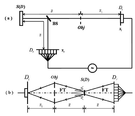
Figure 1: (a). Standard schematic of lensless far-field GI with pseudo-thermal light; (b). the physical explanation of far-field GI, the thermal source $S$ shown in the scheme (a) acts as a phase conjugated mirror and a spatial low-pass filter because of its finite transverse size.

For compressive ghost imaging demonstrated in Ref. Katz , the speckle’s transverse size is small enough to resolve the object and the test detector is positioned at the near field of the object, thus the test detector should be a bucket detector, which can collect the global information transmitted through the object. Fig. 1(a) presents the experimental schematic for lensless far-field ghost imaging. Different from the case mentioned in Ref. Katz , the speckle’s transverse size is too large to resolve the object and the test detector is fixed in the far field of the object, thus a single pointlike detector is enough to record the global information from the object. In the experiment, the pseudo-thermal source $S$, which is obtained by passing a focused laser beam (with the wavelength $\lambda$=650nm and the source’s transverse size $D$) through a slowly rotating ground glass disk Gong , is divided by a beam splitter (BS) into a test and a reference paths. In the test path, the light goes through a double-slit (slit width $a$=100$\mu$m, slit height $h$=500$\mu$m and center-to-center separation $d$=200$\mu$m) and then to a detector $D_{t}$ fixed in the far field of the object (namely $z_{1}>\frac{2d^{2}}{\lambda}$). In the reference path, the light propagates directly to a camera $D_{r}$. Both the object and the camera $D_{r}$ are located in the far field of the source (namely $z>\frac{2D^{2}}{\lambda}$).

The intensity distribution on the detection plane at time $s$ can be expressed as Goodman

$$I_{s}(x,y) = \int{dx_{1}}{dy_{1}}{dx_{2}}{dy_{2}}E_{s}(x_{1},y_{1})E_{s}^{*}(x_{2},y_{2})$$ (1)

$$\times h^{*}(x,y;x_{2},y_{2})h(x,y;x_{1},y_{1}).$$

where $E_{s}(x_{1},y_{1})$ denotes the light field on the source plane at time $s$, $h(x,y;x_{1},y_{1})$ and $h^{*}(x,y;x_{2},y_{2})$ are the impulse function of optical system and its phase conjugate, respectively.

By Ref. Cheng ; Gatti ; Gong , the correlation function for far-field GI shown in Fig. 1(a) can be represented as

$$G^{(2,2)}(x_{r},y_{r};x_{t},y_{t})\propto\left|\right.\int{dx^{\prime}}{dy^{\prime}}T(x^{\prime},y^{\prime})$$

$$\times\sin c[\frac{D}{{\lambda z}}(x_{r}-x^{\prime})]\sin c[\frac{D}{{\lambda z}}(y_{r}-y^{\prime})]$$

$$\times\exp\{\frac{{j\pi}}{{\lambda z_{1}}}[(x_{t}-x^{\prime})^{2}+(y_{t}-y^{\prime})^{2}]\}$$

$$\times\exp\{\frac{{j\pi}}{{\lambda z}}({x^{\prime}}^{2}-{x_{r}}^{2}+{y^{\prime}}^{2}-{y_{r}}^{2})\}\left.\right|^{2}.$$ (2)

where $T(x,y)$ is the object’s transmission function and $\sin c(x)=\frac{\sin(\pi x)}{\pi x}$. From Eq. (2), by the intensity correlation measurements, the best resolution of far-field GI with thermal light is determined by the speckle’s transverse size on the object plane ($\Delta x_{s}\approx\frac{{\lambda z}}{D}$), which is the same as GI in the near field or Fresnel region Zhang ; Ferri .

For far-field GI scheme shown in Fig. 1(a), a single pointlike detector far from the object is enough to record the complete information of the object and its image in real-space can be reconstructed by measuring the intensity correlation function between the two detectors Gong . According to Klyshko’s “advance optics” picture Klyshko , as shown in Fig. 1(b), the object can be considered as being illuminated by a light source emitting the light from the test detector $D_{t}$. After inverse propagating in free space, the Fourier-transform (FT) diffraction pattern of the object will appear in the far field of it (namely the source plane $S$). Because the thermal source $S$ acts as a phase conjugated mirror Valencia and a spatial low-pass filter when the source’s transverse size is finite, only the low space frequency part of the diffraction pattern will be reflected into the reference path. After propagating along the reference path to the far field of the source $S$, the reflected diffraction pattern will be inverse Fourier-transformed and a low resolution real-space image will finally be recorded by the camera $D_{r}$. However, for the case shown in Fig. 1(b), Ref. Donoho has proved theoretically that super-resolution imaging can be obtained by exploiting the images’ sparsity constraints, and CS also utilizes the sparsity constraints of the images in the recovery process while the image extraction process of GI satisfies RIP of CS. Thus, combining GI with CS, superresolved images can be reconstructed by ghost imaging via sparsity constraints (GISC) described next in detail.

To GISC, we formulate it in the CS framework. For the GI system shown in Fig. 1(a), each of the speckle intensity distributions on the detection plane $D_{r}$ at time $s$ is described by $I_{s}(x,y)$ ($n\times m$ pixels) and is reshaped as a row vector ($1\times N$, $N=n\times m$). After $K$ measurements, the random sensing matrix A ($K\times N$) is reconstructed and at the same time, the intensities ($B_{s}$) recorded by the test detector $D_{t}$ are arranged as a column vector Y ($K\times 1$). If we denote the unknown object image as a $N$-dimensional column vector X ($N\times 1$) and X can be represented as ${\rm{\textbf{X}}}={\rm{\Psi}}{\rm{\ }}{\rm{\cdot}}{\rm{\ }}{\rm{\alpha}}$ such that ${\rm{\alpha}}$ is sparse in the representation basis ${\rm{\Psi}}$, then the image can be reconstructed by solving the following convex optimization program Candes ; Figueiredo :

$${\rm{X}}={\Psi\cdot\rm{\alpha}};{\rm{\ }}{\rm{which\ minimizes:}}{\rm{\ }}\frac{{\rm{1}}}{{\rm{2}}}\left\|{{{\rm{\textbf{Y}}}-\rm{\textbf{AX}}}}\right\|_{2}^{2}+\tau\left\|{\rm{\alpha}}\right\|_{1}.$$ (3)

where $\tau$ is a nonnegative parameter, $\left\|V\right\|_{2}$ denotes the Euclidean norm of $V$, and $\left\|V\right\|_{1}=\sum\nolimits_{i}{\left|{\upsilon_{i}}\right|}$ is the $\ell_{1}$ norm of $V$. Therefore, for the image with sparse cartesian representation, the reconstruction process can be clearly written as follows based on Eq. (3):

$$\left|{T_{{\rm{GISC}}}}\right|=\left|{T^{\prime}}\right|;{\rm{\ }}{\rm{which\ minimizes:}}{\rm{\ }}\frac{{\rm{1}}}{{\rm{2}}}\left\|{B_{s}-\int{dx}{dy}}\right.$$

$$\times\left.{I_{s}(x,y)\left|{T^{\prime}(x,y)}\right|^{2}}\right\|_{2}^{2}+\tau\left\|{\left|{T^{\prime}(x,y)}\right|^{2}}\right\|_{1},{\rm{}}\forall_{s}=1\cdots K.$$ (4)

where

$$I_{s}(x,y) \propto \int{dx_{1}}{dy_{1}}{dx_{2}}{dy_{2}}E_{s}(x_{1},y_{1})E_{s}^{*}(x_{2},y_{2})$$ (5)

$$\times \exp\{-\frac{{2j\pi}}{{\lambda z}}[(x_{1}-x_{2})x+(y_{1}-y_{2})y]\}.$$

$$B_{s} \propto \int{dx_{1}}{dy_{1}}{dx_{2}}{dy_{2}}{dx}^{\prime}{dy^{\prime}}{dx}^{\prime\prime}{dy}^{\prime\prime}T(x^{\prime},y^{\prime})T^{*}(x^{\prime\prime},y^{\prime\prime})$$ (6)

$$\times E_{s}(x_{1},y_{1})\exp\{\frac{{j\pi}}{{\lambda z}}({x^{\prime}}^{2}+{y^{\prime}}^{2}-{x^{\prime\prime}}^{2}-{y^{\prime\prime}}^{2})\}$$

$$\times E_{s}^{*}(x_{2},y_{2})\exp\{\frac{{j\pi}}{{\lambda z_{1}}}(x^{\prime 2}+y^{\prime 2}-x^{\prime\prime 2}-y^{\prime\prime 2})\}$$

$$\times \exp\{\frac{{2j\pi}}{{\lambda z}}(x^{\prime\prime}x_{2}+y^{\prime\prime}y_{2}-x^{\prime}x_{1}-y^{\prime}y_{1})\}$$

$$\times \sin c[\frac{{L_{1}}}{{\lambda z_{1}}}(x^{\prime}-x^{\prime\prime})]\sin c[\frac{{L_{1}}}{{\lambda z_{1}}}(y^{\prime}-y^{\prime\prime})].$$

and $\left|{T_{{\rm{GISC}}}}\right|$ is the object’s transmission function recovered by GISC method, $L_{1}$ is the effective receiving aperture of the test detector $D_{t}$.

Figs. 2-3 present experimental results of a double-slit recovered by GI and GISC methods in different receiving areas $L_{1}\times L_{1}$ and different distances $z_{1}$, using the schematic shown in Fig. 1(a). For GISC method, we have utilized the gradient projection for sparse reconstruction algorithm Figueiredo ; Website . As shown in Fig. 2(c-d), the object’s image can not be reconstructed by GI because the transverse size of the speckle on the object plane $\Delta x_{s}$ is much larger than center-to-center separation of the object, which is consistent with the result expressed by Eq. (2) and accords with the physical explanation described in Fig. 1(b). However, the images with the resolution beyond $\frac{1}{6}\Delta x_{s}$ (Fig. 2(e,f)) and Fig. 3(a-d)) can be obtained by GISC. As the receiving areas of the detector $D_{t}$ are increased or the distance between the object and the detector $D_{t}$ is decreased, the quality of GISC will be improved (Fig. 2(e,f) and Fig. 3(a-d)), which can be explained by Eqs. (4-6) because the Euclidean term in Eq. (4) will approach zero such that Eq. (4) becomes the linear $\ell_{1}$-norm problem as the increase of $L_{1}$ or the decrease of $z_{1}$ Candes . Moreover, as shown in Fig. 2(e,f), the resolution of the images reconstructed by GISC also depends on the pixel-resolution of the camera $D_{r}$.

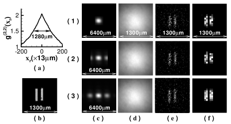
Figure 2: Experimental reconstruction of a double-slit in different receiving areas with $z$=1200mm, $z_{1}$=500mm and $D$=0.6mm (the speckle’s transverse size on the object plane $\Delta x_{s}$=1280mm). (a). The cross-section curve of the speckle on the object plane obtained by measuring the second-order correlation function of light field on the reference detection plane (the curve’s full-width at half-max is the resolution limitation of GI); (b). the object; (c). the object’s diffraction patterns received by the test detector $D_{t}$; (d). GI method (averaged 3000 measurements); (e) and (f) are GISC when the pixel-resolution of the camera $D_{r}$ is 13$\mu$m and 65$\mu$m, respectively (with 3000 and 500 measurements for (e)-(f), respectively). The receiving areas of the detector $D_{t}$ shown in (1-3) are 1.6mm$\times$1.6mm, 3.2mm$\times$3.2mm, and 6.4mm$\times$6.4mm.

Figure 3: Experimental results of the same double-slit in different distances $z_{1}$, and the other conditions are the same as Fig. 2 (using 1000 measurements). (a)-(d) are GISC when the pixel-resolution of the camera $D_{r}$ is 26$\mu$m and $z_{1}$=500mm, 200mm, 100mm and 10mm, respectively. The receiving area of the detector $D_{t}$ is 6.4mm$\times$6.4mm.

To verify the super-resolution ability of GISC for more general images and the effect of the object’s sparse representation on the quality of GISC, as shown in Fig. 4(c) and (e), a transmission aperture (“zhong”ring) with the resolution beyond $\frac{1}{5}\Delta x_{s}$ is reconstructed by GISC in cartesian and DCT representation basis, which suggests that the images with much better quality can be obtained by choosing a proper representation basis. Therefore, for the first time, we demonstrate experimentally that far-field superresolved imaging can be realized by utilizing the images’ sparsity constraints in ghost imaging schemes.

Figure 4: Recovered results of an aperture (“zhong”ring) in different representation basis, with the same conditions of Fig. 3 and $z_{1}$=10mm (using 2000 measurements). (a). The object; (b). GI reconstruction; (c). GISC reconstruction when the object is represented in cartesian basis; (d). the object’s discrete cosine transform (DCT) coefficients; and (e). GISC reconstruction when the object is represented in DCT basis.

In single-photon imaging system, each of the photons only interferes with itself Dirac , it is impossible to obtain the real-space image of a double-slit and its diffraction pattern at the same time because a photon cannot pass both of the slits to generate the double-slit’s diffraction pattern while at the same time pass one of them to give out the double-slit’s image in real-space. For GI, based on the property of spatial correlation between two light fields, it is also impossible to obtain both the image in real-space of the double-slit and its diffraction pattern at the same time in fixed GI schemes Ferri ; Bache ; Basano . However, by taking the image’s sparsity as a priori information, in far-field GISC system shown in Fig. 1(a), when the transverse size of the speckle on the object plane is much larger than center-to-center separation of the double-slit and the test detection plane is located in the far field of the double-slit, the double-slit’s diffraction pattern and its real-space image, as shown in Fig. 2(c) and Fig. 2(e,f), can be obtained at the same time. Moreover, the reconstruction results of GISC don’t only depend on how we measure the object as in a standard quantum measurement frames, but also depend on how sparse the object is in the representation basis (Fig. 3(d) and Fig. 4(c,e)). Actually, for any GI system, we can find a suitable representation basis in which the object is sufficiently sparse, therefore, as shown in Fig. 3(d) and Fig. 4(c,e), super-resolution imaging can be achieved and GISC will be a universal super-resolution imaging method. Understanding what happens at quantum level in GISC seems to be an interesting challenge deserving more investigation.

In conclusion, we have achieved super-resolution far-field GI by combining GI method with the sparsity constraints of images. Both the approaches to realize the linear $\ell_{1}$-norm problem and an optimal representation basis can dramatically enhance the image’s reconstruction quality. We have also shown that Fourier-transform diffraction pattern of the object and its image in real-space can be obtained at the same time. This brand new far-field super-resolution imaging method will be very useful to microscopy in biology, material, medical sciences, and in the filed of remote sensing, etc.

The work was supported by the Hi-Tech Research and Development Program of China under Grant Project No. 2011AA120101 and No. 2011AA120202.

References

- (1) S. Chaudhuri, Super-resolution imaging, (Kluwer Academic Publishers, Norwell, 2001).
- (2) M. I. Kolobov, Quantum Imaging (Springer Science+Business Mediea, LLC, New York, 2007), Chap.6.
- (3) E. A. Ash, and G. Nicholls, Nature, 237, 510-512 (1972).
- (4) S. A. Ramakrishna, Rep. Prog. Phys. 68, 449-521 (2005).
- (5) J. B. Pendry, Phys. Rev. Lett. 85, 3966-3969 (2000).
- (6) J. W. Goodman. Introduction to Fourier Optics. (Mc Graw-Hill, New York, 1968).
- (7) M. Fernandez-Suarez, and A. Y. Ting, Nature Reviews Molecular Cell Biology, 9, 929-943 (2008).
- (8) J. L. Harris, J. Opt. Soc. Am. 54, 931-936 (1964).
- (9) S. G. Mallat, IEEE Trans. Pattern Anal. Machine. Intell. 11, 674-693 (1989).
- (10) B. R. Hunt, International Journal of Imaging Systems and Technology, 6, 297-304 (1995).
- (11) S. R. DeGraaf, IEEE Trans. Imag. Process. 7, 729-761 (1998).
- (12) S. C. Park, M. K. Park, and M. G. Kang, IEEE Signal Process. Mag. 20, 21-36 (2003).
- (13) J. Cheng and S. Han, Phys. Rev. Lett. 92, 093903 (2004).
- (14) A. Gatti, E. Brambilla, M. Bache, and L. A. Lugiato, Phys. Rev. Lett. 93, 093602 (2004).
- (15) R. S. Bennink, S. J. Bentley, R. W. Boyd and J. C. Howell, Phys. Rev. Lett. 92, 033601 (2004).
- (16) W. Gong, P. Zhang, X. Shen, and S. Han, Appl. Phys. Lett. 95, 071110 (2009).
- (17) P. Zhang, W. Gong, X. Shen, and S. Han, Opt. Lett. 34, 1222-1224 (2009).
- (18) F. Ferri D. Magatti, A. Gatti, M. Bache, E. Brambilla, and L. A. Lugiato, Phys. Rev. Lett. 94, 183602 (2005).
- (19) A. Valencia, G. Scarcelli, M. D Angelo, and Y. Shih, Phys. Rev. Lett. 94, 063601 (2005).
- (20) M. D’Angelo, and Y. H. Shih, Laser. Phys. Lett. 2, 567-596 (2005).
- (21) W. Gong, and S. Han, Phys. Lett. A. 374, 1005 (2010).
- (22) F. Ferri, D. Magatti, L. A. Lugiato, and A. Gatti, Phys. Rev. Lett. 104, 253603 (2010).
- (23) H. Liu, J. Cheng, and S. Han, J. Appl. Phys. 102, 103102 (2007).
- (24) M. Bache, E. Brambilla, A. Gatti, and L. A. Lugiato, Opt. Express 12, 6067-6081 (2004).
- (25) L. Basano and P. Ottonello, Opt. Commun. 22, 2741-2745 (2009).
- (26) D. L. Donoho, Siam. J. Math. Anal, 23, 1309-1331 (1992), and references therein.
- (27) O. Katz, Y. Bromberg, and Y. Silberberg, Appl. Phys. Lett. 95, 131110 (2009).
- (28) E. J. Candès, C. R. Acad. Sci. Paris, Ser. I 346, 589-592 (2008).
- (29) E. J. Candès and M. B. Wakin, IEEE Signal Process. Mag. 25, 21 (2008), and references therein.
- (30) M. A. T. Figueiredo, R. D. Nowak, and S. J. Wright, IEEE J. Sel. Top. in Sig. Proc. 1, 586-597 (2007).
- (31) http://www.lx.it.ptmtf/GPSR/.
- (32) D. N. Klyshko, Photons and Nonlinear Optics (Gordon and Breach, New York, 1988).
- (33) P. A. M. Dirac, The Principle of Quantum Mechanics (Oxford, USA, 1930), pp. 9.