A Detailed Far-Ultraviolet Spectral Atlas of Main Sequence B Stars

Abstract

We have constructed a detailed spectral atlas covering the wavelength region 930 Å  to 1225 Å  for 10 sharp-lined B0-B9 stars near the main sequence. Most of the spectra we assembled are from the archives of the FUSE satellite, but for nine stars wavelength coverage above 1188 Å  was taken from high-resolution IUE or echelle HST/STIS spectra. To represent the tenth star at type B0.2 V we used the Copernicus atlas of $\tau$ Sco. We made extensive line identifications in the region 949 Å  to 1225 Å  of all atomic features having published oscillator strengths at types B0, B2, and B8. These are provided as a supplementary data product, - hence the term detailed atlas. Our list of found features totals 2288, 1612, and 2469 lines, respectively. We were able to identify 92%, 98%, and 98% of these features with known atomic transitions with varying degrees of certainty in these spectra. The remaining lines do not have published oscillator strengths. Photospheric lines account for 94%, 87%, and 91%, respectively, of all our identifications, with the remainder being due to interstellar (usually molecular H₂) lines. We also discuss the numbers of lines with respect to the distributions of various ions for these three most studied spectral subtypes. A table is also given of 167 least blended lines that can be used as possible diagnostics of physical conditions in B star atmospheres.

atlases – stars: early-type – ultraviolet: stars –line: identification – atlases

1 Introduction

To understand the physical conditions of O and B stars and their immediate environments there can be no better mode of study than high-dispersion ultraviolet spectroscopy. The spectral energy distributions of hot stars peak in this regime, and it is also here that absorption lines arising from a wide range of excited atomic states appear in high concentration. These lines provide a rich and rather unexplored area for the study of markers of atmospheric temperature, pressure, kinematics, and chemical composition. In addition, atoms undergoing far-UV transitions “see” down to deep layers of the atmosphere because of the local relative transparency. The resulting intense UV radiation field is responsible for creating departures from LTE in these transitions and influencing the calibration of spectral diagnostics. Once atmospheres of single hot stars are understood, this knowledge can be extended to the interpretation of spectra of distant ensembles of hot stars and star formation regions.

At about the turn of this century the era dawned in which specific far-UV spectral lines observed in OB clusters embedded in highly redshifted galaxies can be studied from the ground at optical wavelengths (e.g., de Mello 2000 et al., Pettini et al. 2001, Dawson et al. 2002, Pettini et al. 2002, Mehlert et al. 2002, Croft et al. 2002, Robert et al. 2003, Shapley et al. 2003, de Mello et al. 2004). In the two decades leading up to and including this milestone, enormous progress was made in understanding the atmospheres and origin of OB stars. First came high-resolution spectroscopic observations of the middle-UV during the extended period (1978-1996) of the International Ultraviolet Explorer (IUE) satellite. Next, the 1999 launch of the Far Ultraviolet Spectroscopic Explorer (FUSE), brought access to the far-UV for hundreds of hot stars in the Milky Way and Magellanic Clouds. This era of grand exploration and surveys closed with the decommissioning of FUSE in 2007. The final reprocessing of the FUSE spectra (covering the wavelength region 920 Å  to 1188 Å) now permits the examination of a wealth of homogeneous high-quality material.

For O and B stars one consolidation of these gains was the addition of a fine set of middle-UV and far-UV spectral atlases. Examples of the former are the Copernicus atlas of $\tau$ Sco (Rogerson et al. 1977) and IUE pictorial atlases of O and B stars (Walborn, Nichols-Bohlin, & Panek 1985, Rountree & Sonneborn 1993, Walborn, Parker, & Nichols 1995). Pellerin et al. (2002) inaugurated a second group of digitized atlases with their atlases of O and early-B type stars of all luminosity classes. This work had the goal of exhibiting the general behavior of the strong photospheric lines and the so called UV wind lines with effective temperature T_eff and luminosity class. Valuable supplemental information about the molecular H₂ lines formed in the interstellar medium (ISM) was also provided. From the point of view of stellar researchers, these features contaminate many of the far-UV photospheric lines of most Galactic stars. This atlas was closely followed by a second spectral atlas on OB stars in the two Magellanic Clouds by the same group (Walborn et al. 2002). This work concentrated on the behavior of wind lines with respect to metallicity as well as temperature and luminosity. In addition to these atlases, Blair et al. (2009) have published a compendium of FUSE spectra of hot stars in the Magellanic Clouds. This atlas focused on the identification of far-UV resonance lines arising from the ISM that are sometimes found at multiple velocities. Specialized atlases are now underway for the purposes of displaying the behavior of specific elements in particular types of stars. For example, an atlas depicting lines of heavy metal elements in IUE spectra of late-B and early B stars has recently been published by Adelman et al. (2004).

The first far-UV high-dispersion spectral coverage published for a B star was the Copernicus atlas of $\tau$ Scorpii (B0.2 V; Walborn 1971) by Rogerson & Upson (1977; “RU77”). Rogerson & Ewell (1985; “RE85”) published a detailed tabulation of photospheric and ISM lines identified in this atlas. The RE85 work was undertaken at a time when spectral synthesis tools were not commonly available, and when reliable identifications lay in the hands of a comparative handful of experienced spectroscopists who were also specialists in atomic physics. Even so, in the absence of commonly available spectral syntheses programs at that time, it was difficult to make wholesale line identifications without significant numbers of errors. This situation has changed dramatically in the intervening years with the development of spectral line synthesis tools that make use of extensive atomic line libraries (as well as the organization of the line libraries themselves).

Inspired by the Copernicus atlas, we decided to address the need for the identification of lines in high-dispersion far-UV spectra along the B main sequence. Thus, the first goal of our work is to select and provide far-UV spectral data for main sequence B0 to B9 stars. The atlas spectra should be sharp-lined enough to permit the resolution of a majority of dominant individual atmospheric lines and to provide spectral data products in a common, continuous-spectrum format ranging in wavelength from near the short-wavelength limit of the FUSE regime to the red wing (1225 Å) of Lyman $\alpha$. Such an assemblage requires not only the cojoining of all FUSE spectral detector segments but also (for B0) of second-order scans of Copernicus’s “U1” multiplier, and echelle spectra from IUE or the Hubble Space Telescope Imaging Spectrograph (STIS). This is necessary to extend our coverage from the FUSE long-wavelength limit of 1188 Å  to 1225 Å, as justified below.

Our second goal is to choose three spectra among our atlas sample that capture the low, high, and midpoints of the excitation range of ions in B star atmospheres and to identify all possible absorption lines that make a noticeable contribution to these spectra according to published atomic line libraries. This addition changes the emphasis of the atlas from the classical high-level montage presentation to a “detailed” attribution of the spectral features. Our third goal is to discuss those metallic lines identified from the second goal in the context of diagnostics of effective temperature, luminosity, and heavy element abundances.

This paper is organized as follows. The selection of spectra and the methodology for data conditioning and line identification are set forth in $\S$2. Section $\S$3 displays portions of the atlas and a detailed list of all (several thousand) of our line identifications as well as a list of “clean” lines across much of the B-star domain. We also discuss an example of the important C III 1176 Å  region used as a temperature diagnostic for this spectral type. In $\S$4 we give relevant statistics from our identifications for the B0, B2, and B8 exemplars we call spectral templates. We provide a comparison of our results with an earlier critique of the Rogerson & Ewell (1985) line attributions for the $\tau$ Sco atlas. We finally give commentary on a number of possible spectral markers for physical conditions in these stars’ atmospheres.

2 Preparation of the Atlas

2.1 Spectral coverage

The primary purpose of this atlas is to provide a continuous spectrum from 930 Å  to 1225 Å  of every spectral subtype of a Galactic B-type star near the main sequence. This means that the atlas is based largely but not exclusively on FUSE spectra, a requirement introduces some complications because it necessitates that data from other instruments be used for coverage beyond the long-wavelength limit of FUSE at 1188 Å. This in turn imposes changes at this wavelength in instrumental sampling, resolution, and, most important of all, a shift to a spectrum of a second star that often reflects slightly different physical properties. Our rationale for extending the atlas wavelength coverage is, first, that we wanted to bridge the broad “middle UV” and “far-UV” regimes empirically defined by the coverages of IUE and FUSE ultraviolet explorer missions. One may define this bridge region in practice as the interval between the long-wavelength limit of FUSE coverage and 1225-6 Å,  where the roll-off in sensitivity at short wavelengths commences for the IUE Short Wavelength (SWP) camera. Second, our aim is to include the Lyman $\alpha$ line, which along with higher Lyman members covered by the FUSE detectors, is an important ingredient in determining the radiative and thermal equilibria of a star’s atmosphere and thus its physical structure. Note that the innermost 6-8 Ångstroms in the Lyman $\alpha$ lines are dominated by an ISM component in spectra of B stars located in the Galactic plane (e.g., Bohlin 1975). Thus by extending atlas coverage to 1225 Å  we can ensure coverage of photospheric lines on both sides of the Lyman $\alpha$ line core. Important spectral diagnostics of temperature and ionization are also included in this region, including sometimes strong resonance lines of Si III (1206 Å) and Si II (1193-1194 Å). Finally, the identification of metallic lines in this region may help distinguish spectral lines formed in atmospheres in stars embedded in redshifted galaxies from those of the local hydrogenic Lyman forest.

2.2 Atlas star selection

The selection of atlas stars required that the spectra have high signal-to-noise ratios and exhibit sharp and single lines. Whenever possible, they must also represent normal (solar-like) photospheric abundances and not suffer much ISM absorption (in practice this means E$(B-V)$ $<$ 0.4). To find suitable far-UV spectra we combed through all B-type III-V class material in the MAST/FUSE archive and identified stars with sharp-lined spectra. For coverage above the long-wavelength limit of FUSE spectra, we included spectra from either the IUE or HST/STIS archive. To follow the discussion on specific stars below, the reader is referred to the final list of our selected atlas stars in Table 1.

As a unique case, and being sharp-lined and bright, the star $\tau$ Scorpii is a “ready made” representative of type B0 V. (Note, however, that its wavelength coverage starts at 948.7, and not 930, Ångstroms. We also note that wavelength corrections have been introduced following an Erratum in the original Rogerson & Upson paper.) For other stars we inspected spectral previews of several hundred stars and in some instances the FITS data themselves to make nine additional selections. Spectral types were taken from the Skiff (2007) catalog, which in the case of multiple assignments fortunately showed at most a small range in range of estimated spectral subtypes. Our star selections required a few compromises. Notably, both of our latest type stars, HD 182308 and HD 62714, have peculiar abundances. HD 182308 has been variously classified as B8 V (Floquet 1970) and B9p(Hg)Mn (Cowley 1968). A detailed inspection of its far-UV line strengths confirms that this star’s atmosphere has anomalous abundances consistent with the HgMn class class of peculiar B stars. HD 62714 has been classified as B9/B9.5HeB7Vp: (Houk & Cowley 1975). Because we noticed that some far-UV lines of chromium or manganese appeared anomalous in strength, the classifications of these two stars as chemically peculiar seems appropriate. For purposes of this atlas, we designated HD 182308 as B8 Vp and HD 62714 as B9 Vp. With these exceptions to our stipulated ideal criteria, we list the star selections for this far-UV spectral atlas in Table 1.

The ordering of stars in this table was facilitated by the progression with spectral subtype of the important C III 1176 Å  complex (see discussion in $\S$3.2), strengths of a few Fe-line (principally complexes), as well as the effective temperatures reported by Kilian (1994; for $\tau$ Sco), Glagolevskij (1994), by T_eff values determined by Fitzpatrick & Massa (1999) and Morel & Butler (2006), and by the $uvbyH\beta$ temperature calibration of B stars of Napiwotzki, Schoenbrunner & Wenske (1993). Our selections left an unfilled gap in our spectral subtypes at B7. However, this gap in T_eff is rather small as the temperatures of the HD 182308 and HD 62714 both seem to be slightly high for stars having these spectral subtypes. Reddening (E(B-V)) values, which generally correlate with ISM column density, are taken from several sources in the literature. Values for the bright stars we used for “adjunct” ($>$1188 Å) spectra, are $\leq$ 0.10.

Panchromatic data from the same instrument (Copernicus) were available for only one star, $\tau$ Sco. For the other spectral types we used observations for the same star both below and above 1188 Å  wherever possible. However, as noted in $\S$2.1, we were obliged to provide this extension by using coadded echelle IUE spectra for another star of virtually the same spectral type in the following cases: for type B1 ($\xi^{1}$ CMa), B2 ($\gamma$ Peg), B2-B3 ($\zeta$ Cas), B3-B4 ($\iota$ Her), and B8p-B8 ($\xi$ Oct.) For B5 (HD 94144), B6 V (HD 30122), and (B9p) HD 62714 echelle STIS spectra were utilized. Because the temperature of our B1 star HD 113012 is already nearly as high as $\tau$ Sco (and to exclude it from the atlas would risk instead adopting another spectrum with much broader lines), it was expedient to use Copernicus of $\tau$ Sco a second time to extend the coverage of HD 113012 for the limited range 1188 Å  to 1225 Å. The details of the adjunct spectra are noted as parenthesized, second-line entries in Table 1.

2.3 Data properties and handling

2.3.1 Basic data properties

“Final” data reprocessings of IUE and STIS echelle spectra were completed in 1997 and 2006, respectively. (The recent refurbishment of the HST by the Space Shuttle Atlantis ensure a new generation of STIS data will follow.) The FUSE data were reprocessed with CalFUSE version 3.2 (Dixon et al. 2007) during 2007-8. These spectra were ingested into the MAST archive, and we retrieved them from this facility.

The FUSE spacecraft utlized four independent telescopes and spectrographs. Paraphrasing the FUSE Archival Instrument Handbook (Kaiser & Kruk 2009), each of the telescopes illuminated its own holographic diffraction grating/camera mounted on a Rowland circle spectrograph and fed light to one of two far-UV microchannel plate detectors that illuminated two microchannel plate detectors via LiF and SiC coated mirrors. Each of the detectors recorded spectra from a pair of these optical channels, one each from focused a camera mirror coated with LiF or SiC and therefore optimized for a limited wavelength range. Nearly complete far-UV coverage of the spectrum is provided by two nearly identical “sides” of the instrument, each of which includes two pairs of LiF and SiC detectors. Flux at almost all wavelengths is recorded by at least two segments (the region 1015-1075 Å  is covered in four segments). Table 2 lists in italics the coverages of each of the FUSE detector segments.

Both IUE and HST/STIS data were obtained through large science apertures with an echelle grating optimized for high orders. References for this instrument and data processing are given, respectively, in Garhart et al. (1997) and Kim Quijano et al. (2007).

The spectral resolutions (full width half maxima) of these spectra, as taken from RU77 or the cited data handbooks are as follows: Copernicus 12-15 km s^-1, FUSE 15 km s^-1, STIS 12-15 km s^-1, and IUE 30 km s^-1. Thus, the resolution of these instruments is approximately matched to the rotational broadening criterion we imposed in our star selection.

2.3.2 Conditioning of FUSE spectra

The conditioning steps for FUSE data were comparatively more complex, first, because of the well known nonlinear excursions of the wavelength scale. These effects are largely due to electron repulsion in the detector that can distort the faithful deposition of photoelectrons. Such excursions are typically not robust with time and cannot be modeled reliably. In addition to this, systematic shifts due to the positioning of the star image in a large science aperture are present. A third problem is the presence of optical vignetting (“worms”) across the detector field that caused artificial and uncharacterizable depressions in certain detector segments, particularly the LiF 1B segment (see Chapter 4 of the FUSE Instrument Handbook; Kaiser & Kruk 2009). Because several instrumental idiosyncracies appear in FUSE detector Sides 1 and 2 spectra, most researchers have learned to work with the segments of these two sides separately and compare them in the end as if they were independent observations. We will do the same here, as we describe the steps to our building two cojoined spectra from the 4 detector segment pairs.

In almost all cases multiple exposures had been taken of our target stars. Therefore, for each of the eight detector segments our first conditioning steps were to cross-correlate to the nearest pixel, co-weight, and add the individual spectral exposures. Coweighting was implemented by means of a simple pixel-to-pixel fluctuation metric used to compute signal-to-noise ratios (Stoehr 2007). In this coweighting step we omitted any spectra (e.g., resulting from incorrect pointings) with weights less than ${\frac{1}{3}}$ the of the maximum weighted observation. Visual inspection then verified that all spectra had been shifted to the nearest pixel of the fiducial (first) observation in the series.

Except for linear interpolation over subpixel scales noted below, our only modifications to the fluxes were to substantially remove the flux depression due to the worm in the region from 1130 Å  to 1160 Å  of the LiF 1B segment. This was done by passing a high order filter having the same degree over the 1B and 2A segment fluxes and then interpolating to the original pixel scale. The 1B worm was “removed” by dividing of the 2A spectrum polynomial fit by the 1B fit in the wavelength region affected by the worm and applying the quotient to the original 1B spectrum.

It was necessary to devote considerable attention to our correction of the wavelength scale. The raw wavelengths exhibits frequent departures of 0.03 Å  or larger from linearity over occasionally even a few Ångstroms. This was accomplished by first determining a trial linear wavelength calibration (generally, by a small, and always subpixel, shift of the spectrum) to match computed Lyman and Werner transitions from a single rotational state of the zeroth vibrational level to the ground state of molecular H₂ lines in the interstellar medium (ISM). The parameters of these transitions were provided by an on-line tool created as part of the “H2ools” project (McCandliss 2003). This tool allowed us to identify these molecular ISM features in all our spectra and and to coplot them on a common wavelength scale. Our procedures permitted us to detect wavelength scale nonlinearities and correct them by imposing shifts on a subpixel scale (0.01 Å) over adjacent wavelength segments to bring the observations into conformity with the theoretical H₂ line “comb.” This procedure was repeated for all segments of the two FUSE detector sides. (We caution the reader than some departures over small wavelength regions as large as ${\pm 0.02}$ Å  may yet exist, although we have tried to correct them all.) As a last step for conditioning FUSE data, we corrected the wavelengths for the most recent stellar radial velocity tabulated in SIMBAD. The final spectra were resampled linearly to the original uniform mesh of the original observations, which for FUSE is 0.013 Å  pixel^-1. The long wavelength ($>$1188 Å) sampling is 0.031 Å  pixel^-1 for IUE, and 0.0052 Å  pixel^-1 for STIS. The wavelength spacing for the far-UV region of the Copernicus atlas is about 0.022  Å  pixel^-1. The original wavelengths and counts from RU77 were used in our re-presentation of their atlas.

Next we cojoined the spectra, both below the demarcation wavelength 1188 Å  (FUSE) and above it. The first step consisted of cojoining the Side 1 spectra, consisting of segments SiC 1B, LiF 1A, SiC 1A, LiF 2A and LiF 1B (where LiF 2A was used to plug a 4 Ångstrom gap in the Side 1 coverage). We spliced these segments at wavelengths where no conspicuous lines are present in our template B0, B2, or B8 spectra. The wavelengths of the FUSE spectra are given within parentheses in Table 2. The spectra for each of the two FUSE sides are cojoined with the IUE or STIS spectra, preserving the original uniform wavelength spacings and adopting a scale factor for the long wavelength spectrum that provides a continuity in flux across the 1188 Å  demarcation.

As an aid to users of the atlas data, we denote those wavelengths for which ISM lines have important contributions, particularly for the atomic and molecular hydrogen features in the spectrum that can be contaminated by absorptions from interstellar gas. These lines often merge together in aggregates covering a few Ångstroms. We located these wavelength regions by selecting a high-quality spectrum with a mixture of broad photospheric and contrasting sharp ISM lines. We used a coaddition of 71 FUSE exposures of HD 195965 (B0 V; E$(B-V)$$\approx$ +0.41; Sasseen et al. 2002) as an ISM line template. We modified the ranges of the spectra for each of the atlas stars and forced the ISM-dominated windows to be the same between pairs of spectral segments covering the same wavelength ranges.

As a last step in constructing spectra over broad wavelengths, we spliced IUE and STIS echelle order segments to the segment-merged FUSE spectra. Splice points were selected at wavelengths where the local noise fluctuations of the neighboring orders were approximately equal. For the IUE spectral spectments we made splice points at 1188.0, 1192.5, 1205.5, 1215.5, and 1225.0 Å.  For STIS the splice points were more closely spaced, about every 3.5 Å,  again starting at 1188.0 Å.

2.4 Tools for line identifications

2.4.1 The three template spectra

We selected as templates, that is representatives from which to identify lines over the B spectral range, the spectra of $\tau$ Sco (B0), HD 37367 (B2), and HD 182308 (B8p). We chose HD 182308 rather than the cooler HD 62714 because the lines of HD 182308 are narrower. We used an effective temperature of 13,100 K to compute synthetic spectra for our cool-star template as this is close to the mean of the T_eff values of these two cool stars (Table 1). Likewise, because the lines of $\tau$ Sco are among the narrowest of any nearby early B star, we chose this as our representative B0 type. Despite the uncalibrated nature of its linearized fluxes, the spectral resolution and signal-to-noise ratio, of the Copernicus spectrum rival or exceed the quality of the FUSE material. We determined from our spectral synthesis model tool that the transition between the dominance of Fe III lines to Fe II lines occurs at about 23,000 K. This is about the expected surface temperature of a B2 V star. Accordingly, we chose the HD 37367 spectrum as our middle-ionization template spectrum. We emphasize that the temperatures chosen for our three spectral templates serve only to identify observed lines and not fit them quantitatively.

2.4.2 Construction of the line library

To prepare for the identification of lines in our spectral templates, we compiled a line library from three sources: the Kurucz (1993) line library, the Vienna Atomic Line Database (“VALD”; Piskunov et al. 1995, Kupka et al. 1999), and the on-line atomic line database of van Hoof (2006). The Kurucz line library has the advantage of being comprehensive and theoretical, meaning that its coverage is not compromised in the far-UV by absorptive optical coatings. However, this list has become dated. The VALD and van Hoof databases are periodically updated and both present a recommended oscillator strength (log $gf$) value for a line if more than one have been published. The VALD library is supported by an interactive web form. The form allows the user to state the stellar effective temperature and a line depth threshold criterion, e.g., 1% line depth, above which lines will be included in a returned list. We exercised this option, and chose T_eff = 23,000 K in our requests. The van Hoof library is likewise extensive and is convenient to use on line, especially during our frequent manual cross-checking of best identifications. Our library did not screen out lines of highly excited ions from the Kurucz atlas contribution. For completeness, we note that Howk et al. (2000) have suggested empirical revisions to log $gf$’s of several Fe II resonance lines in the range 1050 Å  to 1150 Å  on the basis of fittings of ISM lines in FUSE spectra. However, the corrections they recommend are generally within a factor of two of the log $gf$ values in our assembled line library. Such corrections have little bearing on the identification of saturated features and could be disregarded. We were able to combine these three line lists and excise duplicate entries listing the same ion and nearly the same wavelength and atomic level excitation. The latter actions were performed by a computer program. However, because the tolerated differences of wavelengths and excitations for the same line could vary by ion, some duplications were identified and excised/ manually. In cases of duplicate entries with the Kurucz list, we exercised a preference for the van Hoof or VALD log $gf$’s and wavelengths.

2.4.3 Line synthesis

All our line identifications were based on our now well defined line library, thereby requiring all these lines have either measured or published log $gf$ values in the literature. In order to make line identifications we used a line annotation facility in the spectral line synthesis program ‘SYNSPEC of Hubeny, Lanz, and Jeffery (1994). This program can be run interactively to compute and plot spectral fluxes over a specified wavelength range once the user specifies key input parameters such as metallicity (assumed to be solar), stellar effective temperature T_eff, log $g$, and microturbulence. In our models we used log $g$ = 4 and $\xi$ = 2 km s^-1. The T_eff values were models closest in integral kilokelvins to the numbers in Table 1. We compared line synthesis results from standard Kurucz (1990) and non-LTE models calculated by TLUSTY from the so-called “B2006” grid (Lanz & Hubeny 2007). The line strengths produced from the two sets of models typically differed by amounts equivalent to a temperature change of 1,000 K for models having a T_eff appropriate to $\tau$ Sco and much smaller than this for a model appropriate to type B8 model. For the purposes of line identifications either set of models would serve just as well for the B8 model. In this case the low precision of log $gf$’s far outweighs uncertainties in the atmospheric T($\tau$)’s in the computed line strengths.

2.4.4 Line identification methodology

In the last several years a few middle-UV spectral atlases have been published with annotations for most visible spectral lines (e.g., Leckrone et al. 1999). We attempted as a key part of our “detailed atlas” to extend this philosophy by identifying all atomic lines responsible for far-UV absorptions in B0, B2, and B8 main sequence spectra (and presumably for subtypes in between). We set the short-wavelength limit of our identification list no shorter than at 949 Å,  the starting wavelength of the RE85 line list, because little purpose would be served by attempting to identify photospheric lines to the blue of this limit, where H and H₂ lines blanketing dominates. The particular challenge faced in the far-UV is the blending of closely spaced lines that cannot be resolved even in stars with rotational broadenings no larger than the IUE instrumental width of about 30 km s^-1. Our procedure was to compute spectral line models in narrow wavelength intervals, often no larger than 3 Ångstroms, and to overplot the synthesis and the identifications provided by SYNSPEC. Manual intervention was often required in the working version of the line list for the following reasons:

• some lines cannot be identified with certainty according to their published log $gf$ values. This is because some $gf$s are too small and they underpredict the line strengths, just as others are too large. Our procedure in such cases was first to seek the best candidate line, next to artificially increase its log $gf$ by a factor of 30 in our working line list, and finally to rerun the SYNSPEC synthesis. If the line appeared in the new synthesis, it was marked as an uncertain identification with a symbol “:” in our compiled line identification lists and figures.

• more than one line might appear as a candidate line within our adopted resolution wavelength window: ${\pm 0.025}$Å  for B0 and ${\pm 0.0375}$Å  for B2 and B8, values ultimately set by the instrumental resolutions and our chosen limit of acceptable rotational broadening (30 km s^-1). Typically, in such instances we temporarily deleted lines from our working line list and determined the relative strengths of the contributors, if necessary one by one. If they contributed by more than 50% of the dominant line in the blend, we retained it. We refer to secondary lines identified within a wavelength window defining a blend a “line group,” and the dominant contributor is the “primary” line (sometimes by a very small amount). Non-dominant contributors are called “secondary” group members. We counted lines as members if their equivalent widths (computed as an isolated line in SYNSPEC and with respect to a continuum determined by this program) was greater than the 50% criterion just noted. In practice, almost all detectable far-UV lines are saturated. Thus, lines contributing less than the primary line’s absorption do not contribute much to a line group’s aggregate strength. We noted the relative equivalent widths of the secondary contributors, and our notes are available upon request.

• a candidate line’s published wavelength differed from the measured flux minimum value by more than $\pm{0.03}$Å.  In some cases, especially for O II, we suspect this threshold should be relaxed to $\pm{0.04}$Å. It is important to note that this limit does not automatically apply to two or more lines separated by more than the wavelength resolution bin value in nearby pairs of blended lines. Thus, sometimes when an array of neighboring candidate lines is included in our identification tables, the wavelength of the primary line does not closely coincide with the minimum of the blended feature.

We note that our line list also includes overpredicted lines, that is, identifications predicted from SYNSPEC with no visible counterparts in the observed spectrum.

The construction of our line list proceeded after first putting into place semiautomated error checking procedures. One such procedure was to check the ion and wavelength values against those in our line library. Our program reported any errors in this collation, and they were corrected. The monotonicity of the wavelengths in the list was likewise checked. Nonetheless, we cannot claim that our list of identifications is error-free! The influences of some lines may yet have been over- or underestimated. Second, we have checked our line identifications with other published lists of prominent far-UV lines, including those in the Pellerin et al. (2002) atlas and the far-UV Capella atlas (Young et al. 2001). We noticed minor deviations in quoted wavelength values for several lines, and in a few cases we could not authenticate line identifications because we could not find log $gf$ values in their secondary sources. The absence of any significant discrepancies in these comparisons suggests that there are few or no gross or systematic errors in our list. In all we believe our identified and unknown lines form a list of all essentially all the visible features that contribute the far-UV absorption lines of B0, B2, and B8 Galactic main sequence stars, including most ISM lines.

3 The atlas

3.1 The atlas and associated data products

This presentation of our “detailed atlas” is different from that of most other atlases. Typically, spectral atlases present a pictorial montage of all spectral types over the full wavelength range surveyed. Our atlas consists of three core products: (1) extensive line identification lists, (2) a graphical plot of line identifications of the three template spectra and, (3) data files containing merged spectra in Flexible Image Transport System (FITS) format. The paper journal version of this work gives an abbreviated representation of the spectral plots and of the identification table. The electronic edition provides the full identification tables both in ASCII text and Excel “xls” format. A copy of our compiled line library will also be provided upon request. In addition to these published venues, all products for this atlas are to be placed in MAST’s “High Level Science Product” (HLSP) area (http://archive.stsci.edu/prepds/fuvbstars/), where the products are further vetted by MAST staff for clarity and ease of access to the astronomical community.

Our detailed line lists for the three B0, B2, and B8 template spectra are presented in Table 3. The table is divided into three subpanels a-c. Each subpanel first lists the star number for which a line has been identified (“1,” “2,” and “3” correspond to spectral types B0, B2, and B8, respectively), then in two columns the identified wavelength from our line list sources, and finally the ion identification. The two wavelength columns represent either the “primary” or “member” (secondary) of a line group, respectively, such that one of the columns is always unfilled. Here “group” refers to a common resolution window in which the wavelength of the primary line is located. We found as many as 7 secondary group members associated with a primary line according to this definition. In addition to “uncertain” identifications referred to earlier, lines for which no extant identification and/or log $gf$ are unavailable are represented in our table with the ion symbol “UN I” for ”unknown.” Wavelengths for H2 identifications were taken from H2ools. The ion column also designates lines that may appear both in the photospheric and ISM spectra of the template stars with the symbol “pism.”

The rows of Table 3 are sorted according to the primary line wavelength of each group and are interleaved among the three template spectra. In the interest of portability the on-line version gives these as a separate table for each template star. Secondary group members follow their associated group primaries, even if the secondary’s wavelength is slightly smaller than the primary’s. A glance at the beginning of Table 3 suggests a trend that is indeed born out by the full listing across the whole far-UV range: 35 of the first short-wavelength lines on the first page are contained in the B0 spectrum. This same page contains only 17 lines identified for the B8 star. The reverse is also true at the longest wavelengths, although less markedly.

Table 4 is a list of 167 least contaminated lines that, typically, are visible in two or all of our template spectra (omitting hydrogen Lyman lines). The excitation of the lower level of these transitions is given in electron Volts (eV) in the fourth column of each of the three subpanels.

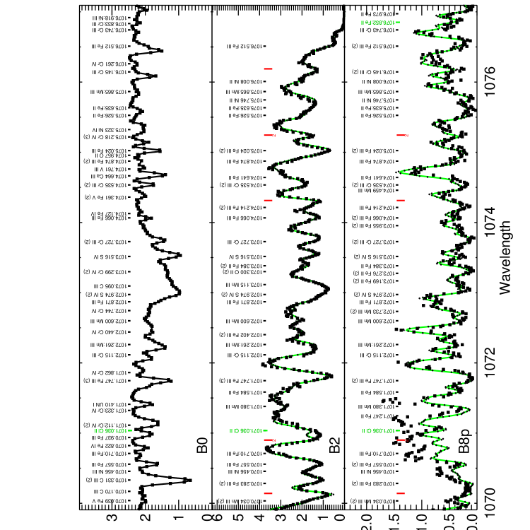
Figure 1: A three panel representation of the atlas and line identifications for main sequence B0, B2, and B8p spectra in the region 1070 Å  to 1177.5 Å. Solid lines in the B2 and B8p panels represent a filtered FUSE spectrum taken from Side 1 detectors; small squares represent Side 2 data. Line identifications are represented vertically by ion and wavelength and, where necessary, with colons to represent uncertainties. Notations such as “(3)” represent the combined number of primary and secondary lines in a wavelength resolution bin. Green annotations represent atomic lines having mainly ISM contributions, and red vertical ticks represent ISM H₂ features. The latter may also have numbers underneath them too if they are primaries in local wavelength groups. The ion “UN I” represents an unidentified absorption line. Copernicus count rates (B0: $\tau$ Sco) are in units of 10⁴, and FUSE fluxes in the B2 and B8p spectra are represented in units of 10^-11 ergs s^-1 cm^-2 Å^-1.

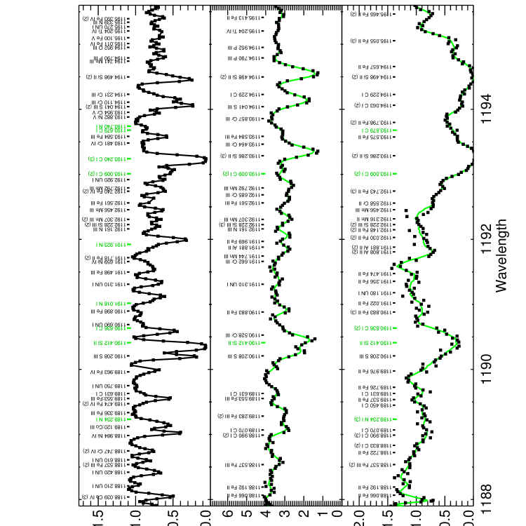
Figure 2: A three panel representation of the atlas and line identifications for main sequence B0, B2, and B8p spectra in the region 1188 Å  to 1195.5 Å, just above the cut-off of FUSE spectral coverage. This figure is a continuation of Fig. 1 but displays spectra recorded from instruments other than FUSE.

Figure 1 is a three-panel representative montage of the three template spectra with line identifications in the almost arbitrarily chosen region between 1070 Å  and 1077.5 Å. A more extended wavelength coverage would render the detailed line identifications difficult to read. This spectral region is not highly contaminated by ISM H₂ features, as it would be below 980 Å, but it also shows a small sample of them. It also exemplifies the occasional scattered light effects that affect the edges of spectral segments (in this case SiC2B). Above 1148 Å  the H₂ lines are no longer present in the spectra. The region shown in Fig. 1 highlights the changes in line identifications while also including a few common lines for visual reference. Similarly, Figure 2 is the first in a series of montages of the three adjunct spectra, again, in the region immediately above the 1188 Å  demarcation. The top panel continues to show the Copernicus spectrum of $\tau$ Sco, while the second and third panels show the IUE spectra of $\gamma$ Peg and $\xi$ Oct. This spectrum highlights the appearance of the Si II 1193 Å  and 1194 Å  resonance lines, which grow in strength from B2 through the remainder of the B spectral sequence. A series of amorphous C I lines, largely formed in the photosphere, can be seen in the lower panel. This is an example of the lowering of the typical ion state seen at the long wavelength end of the atlas. The green line in these figures are 4-point filtered averages of the Side 1 spectra.

Line annotations are given in Figs. 1 and Fig. 2 for the group primary lines only. The number in parenthesis following the annotated identification corresponds to the total number of group members (whether photospheric or ISM). For example, “(2)” means the line group consists of the primary and one secondary contributor. In cases where the primary line is a H₂ line this number is also indicated, but without parentheses under the indicated red line segment. Also, atomic ISM lines are annotated in the color green. The electronic version of this paper contains a full set of three-panel spectral plots, covering our full spectral range, similar to Figs. 1 and 2.

The FITS products available through MAST are two-extension binary table files. Each extension contains data for a FUSE detector side as well as salient details about the observation (only one extension is needed for the single Copernicus atlas spectrum of $\tau$ Sco). The first FITS extension contains FUSE Side 1 data as well as data for wavelengths above 1181 Å.  The spectral data are arranged in three columns consisting of wavelengths, fluxes, and an integer flag with value 0, 1, or 2. Fluxes at wavelengths shorter than 1188 Å  have a flag value 0 if they are formed mainly in an ISM feature,, a value 1 if they are formed mainly in the photosphere, and a value 2 (Side 1 only) if they are associated with a wavelength greater than 1188 Å  and come from an observation of a star other than the star oberved for wavelengths below this limit. Full coverage plots can be made either by ignoring the flags or coplotting each set of segments with with their separate flag codings. The wavelength and flux vectors are in native units (wavelengths in Ångstroms, fluxes in ergs s^-1 cm^-2 Å^-1). The FITS files also contain header keywords that include the names, spectral types, and E(B-V) reddening (if available) of the stars used, the dataset ID sequences, number of exposures, scaling factor to bring long wavelength ($\geq$1188 Ångstroms) fluxes into agreement with the short wavelength fluxes, start and end times of observations, and total exposure time.

3.2 Example: the C III 1176 Å  region

We exhibit as Figures 3 and 4 a montage of 8 of the 10 atlas spectra in the region of the C III 1176 Å  complex. This aggregate consists of a series of six primary C III lines arising from levels at $\chi$ = 6.5 eV. Annotations of the ions responsible for primaries in most line groups are given for the three templates in Fig. 3 - at the top for B0 and at the bottom for B2. These annotations are staggered even-odd vertically in the figure so as to make the identifications readable. In Fig. 4 the line crowding is severe enough that we were obliged to display line identifications for B8 alone. In this case the two rows of annotations alternate at the top and bottom of the plot. These figures demonstrate that the C III complex forms a useful diagnostic not only for early B types but for late B stars as well. However, we note that the precise positions of individual components become shifted by blends from nearby Fe-group line blends. The 1176 Å  region is an especially instructive example of the interplay of carbon and heavy element lines. At least a few lines in this wavelength region remain visible through all B types (e.g. Cr III 1182 Å) or at least at the early or late ends of the B domain (e.g., for B0-B8: N I 1172 and 1177 Å; for B5-B9: C IV 1169 Å  and Si III 1182 Å). Some of these indicators, such as a pair of weak C III and C IV lines, are visible to earlier types. In fact, from a few O star spectra examined outside our atlas sample, we discovered that various C III lines in the wavelength interval shown in Fig. 3 can form a diagnostic for differentiating between late O spectral types and also between main sequence and giant stars (see $\S$4.3).

4 Discussion

4.1 Line statistics

The number of lines found in our spectral templates for B0, B2, and B8p is 2288, 1612, and 2469, respectively. Of these, 7.9%,, 2.1%, and 2.2% could not be identified from our line library. The percentages of lines that are overpredicted are 12.5%, 5.5%, and 5.6%, respectively. Conversely, similar percentages, namely 13%, 7%, and 6% of our found features, have “uncertain” (low log $gf$) criterion. We expect that the great majority of these are actually valid identifications and their log $gf$s are too low. For example, random spot checks of the log $gf$’s required to match the observed strengths with our spectral syntheses suggest that the log $gf$ error distribution is likewise consistent with a broad Gaussian with two approximately equal “weak” and “strong” tails.

Photospheric lines account for 93.7%, 87.0%, and 91.3% of the identifications in the respective templates. The few percent complement of these are due to ISM features, which become increasing numerous with decreasing wavelengths. For example, shortward of 1148 Å, we identified a total of 200 H₂ lines that are either dominant or secondary contributors to absorption features. Of these only two identifications are clearly H₂ primary lines in the $\tau$ Sco spectrum, a star located along the “Scorpius ISM tunnel.” More typically, H₂ lines comprise the overwhelming contribution of the ISM component in our B2 and B8p template spectra and account for the lower two percentages (87.0%, 91.3%) for these cases compared to the overall identification rates.

As to photospheric features, we made a total of 5800 photospheric atomic line identifications in the three template stars, of which 4216 are unique. We expect that synthetic photospheric and ISM spectra could be computed solely from this list of unique lines. This also means that altogether our list includes 13.7% of our adopted line library tabulations over its range of 949 to 1225 Å. We believe this high rate (particularly considering the inclusion of excited ions in our line list) speaks to the general success of our identification efforts. We estimate that this percentage would be as high as 15-16% if we excluded wavelength regions blanketed by saturated resonance, hydrogen, or H₂ ISM lines.

From our line statistics we find a few trends with spectral type. The first of these is the a comparatively high rate of uncertain identifications and nonidentifications for B0 spectral features, suggesting an incompleteness in log $gf$’s for transitions arising from thrice ionized Fe-group elements. However, at least part of this is likely a residual of the problem that interfered with the identification efforts by RE85. Many of RE85’s still unconfirmed identifications may well prove to be correct at some future point when quantitative measurements of these lines are made.

A second trend with spectral type is in the number of far-UV photospheric lines identifed across the range of B spectra. We found a local minimum at type $\sim$B2 in the number of detected lines. Some 20-25% of the comparative dearth of identifications at type B2 arises from obscuration of photospheric lines by the larger wavelength regions dominated by strong ISM H₂ and photospheric resonance lines arising from ions like Si III. The rest of this dearth is a consequence of the ionizations changing from thrice and single ionization states to second ionizations as one moves toward B2 from B0 and B8. Thus, the addition of lines of twice-ionized states does not compensate for the loss of lines from the other two ion stages. An additional detail is that over 91% of the identified photospheric lines in the B2 spectrum are also visible (as primary or secondary lines) in either the B0 or B8 spectrum. Conversely, some 67% and 53% of the lines in the B0 and B8 spectrum are not visible in the B8 and B0 spectrum, respectively. Some 608 primary or secondary lines remain visible across the entire B main sequence domain.

A third trend is that the percentage of isolated primary lines in resolution wavelength bin groups declines dramatically across the early B spectral range (from 81% at B0, 66% at B2, to 59% at B8p) and also with decreasing wavelength. Some of these “isolated” primary lines are barely resolved, and these can be utilized only in a sharp-lined spectrum. For this reason the list of least contaminated lines (Table 4) runs to only 5% of the total line list.

The general expectation that the Fe- group lines dominate the far-UV spectra of hot stars is borne out by our identifications. Indeed iron itself dominates this population. Numbers of iron lines identified in the associated ion stages are exhibited in Table 5. Lines of chromium, followed closely by manganese, are a distant second to the incidence of iron lines.

4.2 Previous critique of Rogerson-Ewell identifications in $\tau$ Sco atlas

Cowley & Merritt (1987; hereafter “CM87”) employed Monte Carlo techniques to test for the presence of several ions identified in the $\tau$ Sco atlas by Rogerson & Ewell (1985). CM87 have critiqued RE85’s claims that lines of certain ions in particular are present in this spectrum. Here we offer comments on these differences based on our own identifications specifically in the region 949 Å  to 1225 Å:

N II:  CM87 questioned whether excited N II features are present. However, since they did not list the earlier claimed identifications by RE85, we cannot address their objections directly. Overall, we found 6 excited lines from this ion in our photospheric syntheses (including 3 resonance lines apparently not in dispute). Since these excited N II lines arise from levels at 13.5 eV, they can hardly be ISM lines. Thus, the presence of photospheric N II lines in this star’s far-UV spectrum is likely.

N I:  Our SYNSPEC syntheses predicted no detectable N I photospheric resonance lines. This implies that features found at these wavelengths are formed in the ISM. However, the photospheric syntheses also predict 8 or 9 N I lines (one is designated uncertain). All of these arise from levels at 3.6 eV. Therefore at least several photospheric lines from this ion are likely to be present in the far-UV $\tau$ Sco spectrum as well as later types. Lines with this excitation potential are generally not primarily formed by the ISM, but we cannot rule out a secondary contribution.

Ne II:  RE85 noted that most of their identifications of Ne II lines are blended features. One of these is the line at 1181.3 Å.  We confirm this, the only possible detection of this ion. Nonetheless, we have designated 1181.3 Å  as an uncertain identification.

P IV:  CM87 reported that identifications of lines of this ion were insecure in this spectrum. However, we found 17 lines as P IV in our photospheric syntheses, all but one of which we consider are likely identifications. In addition, we confirm the detection of at least two P IV lines in the IUE wavelength range that CM87 considered “marginally significant.” We were able to do this on the basis of many more IUE observations made subsequent to the CM87 study. The presence of this ion is secure.

P III:  CM87 questioned RE85’s claim of 91 P III lines in this spectra. In the far-UV, we found only four lines of this ion. Of these only 1184.2 and 1194.7 Å  are excited lines. Because these features are among the strongest predicted subordinate lines for this ion in our spectral syntheses, we are able to confirm the identification in strong P III lines in the photospheric spectrum.

S II:  CM87 agreed with RE85 that lines of this ion are present, but not on the basis of as many lines they claimed. We identified only 4 lines for this ion, of which 2 are marked “uncertain.” The presence of this ion is probably secure, but (as also for P III) there is at best a marginal hope of using the few available S II lines for diagnostic purposes.

Mn III:  CM87 stated that they found “marginal support… for the presence a few of the strongest Mn III lines.” They suggested that a future study might find the abundance of this element to be subnormal. However, we have identified 135 lines of this ion in the same spectrum, of which no more than ${\frac{1}{3}}$ are uncertain identifications. The presence of this ion in this spectrum is certainly secure.

Zn III:  Like CM87 we are unable to confirm identifications of this ion in the far-UV.

4.3 Temperature and chemical Indicators

In this section we indicate lines that may be used in far-UV spectra of sharp-lined B stars near the main sequence to refine diagnostics of effective temperature, chemical composition, and occasionally log $g$. For the B V stars most of the interesting abundances are likely to relate to products of the CNO-cycle and to evidence of Bp compositional anomalies, usually Si, Cr, and/or Mn. However, we include lines of other elements that may serve as metallicity indicators.

In our descriptions below we give weight to the “clean” spectral lines listed in Table 4. However, we also include some lines that have minor blend contributions if they are present over a range of spectral types. We made our judgments by explicitly surveying the B0, B1, B2, B5, B8, and B9 spectra from this atlas. In general, those lines of singly-ionized species exhibit the greatest variations in strength along the B sequence. Lines arising from thrice-ionized atoms, except for abundant elements like silicon, generally exist only in at types B0 and B1. Those lines exhibiting the smallest changes in equivalent width have moderate excitations (4-8 eV) of doubly ionized atoms - a delicate balance between excitation and ionization effects. Being least sensitive to changes in photospheric temperature, and not being sensitive to wind conditions, these lines are the best indicators of abundance. We prefix below the ion name of Si IV with an asterisk because the members of the UV resonance doublet (1394 Å, 1403 Å) exhibit an obvious wind component in the great majority of early B-type spectra. Because wind lines can be strongly contaminated by both emission and absorptions deeper in the star’s atmosphere, lines listed for Si IV are especially valuable diagnostics of temperature and/or abundance.

Reasonable ionization criteria can often be framed from the following ion ratios in our B star atlas spectra: carbon (IV/III/II/I), nitrogen (IV/III/II/I), oxygen (III/II/I), silicon (IV/III/II), phosphorus (V/IV/III/II), sulfur (IV/III/II), chlorine (III/II), chromium (IV/III/II), manganese (III/II), iron (IV/III/II), and cobalt (II/II). In those cases where lines of three ion stages can be detectable, all three are generally visible only down to types B1 or B2. Exceptions to this statement are silicon and sulfur. For these elements lines of three ionization states may be found in spectra for type B5 and even later.

We list lines in order of ion atomic sequence that are usually visible in two of our three major template spectra (B0, B2, and B8) and which usually can be found in our Table 3. Lines that appear in only our B0 or B0-B1 spectra include He I 958.6 Å, C IV 1107.5 and 1168.9 Å, P V 1117.9 Å, 1128.0 Å, and Ca III 1116.0 Å. Pellerin et al. (2002) have discussed the special case of He II 1084.8 Å  line, whose diagnostic value is compromised by blends of N II lines. We will not repeat these in the following ion listing.

C III:  The feature at 977.0 Å  is a well known pressure-sensitive resonance line in B spectra, although in practice its profile in Galactic B star spectra is marred by the appearance of molecular H₂ lines (Pellerin et al. 2002, Walborn et al. 2002). Nonetheless, researchers can make use of this line along with the C III 1176 Å  complex to determine both an early B star’s spectral type and luminosity class, particularly in Magellanic Cloud stars well out of the Galactic plane (e.g., Walborn et al. 2002). As noted in $\S$3.2, the weak C III line complex between 1165.6 Å  and 1165.9 Å  extends from O8 to B1-B2 on the main sequence.

C II:  Strengths of the subordinate (9.6 eV) 961.2, 972.3, and 996.3 Å  lines of this low-ionization species increase slowly and persist through B-types. Strengths of the high excitation (13.7 eV) 1138.9 and 1139.3 Å  lines persist to B5 before weakening to invisibility. Lines at 1009.9 and 1010.3 Å  attain maximum strengths at B2-B3, but they then decrease slowly and are still visible at type B8.

C I:  A resonance feature, 1135.8 Å  is the only line clearly visible across all the B subtypes. A second resonance line at 1138.5 Å  appears at B2 and remains visible for A types and later.

N IV:  The high excitation 1131.4 Å  feature is visible from at least O9 through type B1. This appears to be a good indicator of T_eff above 25,000 K. However, note that this line is contaminated by O III 1131.0 Å, which also fades at about the same rate as N IV. It is absent by type B2.

N III:  The N III complex near 979.8 Å  fades very fast with spectral type. As noted by Pellerin et al. (2002), the lines at 987.7 and 991.5 Å  fade into nearby atmospheric or H₂ blends at type B2, and 1184.5 Å  does so at $\sim$B5.

N II:  The features at 1083.9 Å  and in the range 1085.5 Å  to 1085.7 Å  are resonance lines that undergo a maximum strength at about B2 and remain visible at B8.

N I:  The photospheric N I lines at 1099.0, 1172.0, 1177.6, and 1200.2 Å  have excitations in the range 0-3.6 eV and increase rapidly with spectral type. The 1184.2 Å  line first makes its appearance at type B5 and strengthens at least to early A star spectra. Of all the N I lines 1200 Å  is the cleanest in our atlas spectra.

O III:  All five lines from this ion are highly excited and decrease to only marginal detectability at B2. These are at 1016.7, 1149.6, 1157.0, 1196.7, and 1199.9 Å. Of these 1199 Å  is the least blended and most suitable for quantitative measurement in early B spectra. Pellerin et al. (2002) have noted the utility of 1149 Å  to hotter stars and particularly in oxygen-rich WC stars.

O II:  Only one line, the high excitation line at 1130.1 Å, remains visible through the whole spectral range, attaining a maximum at about type B8.

O I:  The line O I 990.2 Å  is visible in all our templates. For the $\tau$ Sco spectrum the feature is probably a photospheric/ISM blend Lines at 1041.6 and 1127.4 Å  appear at B2 and steadily increase in strength.

Al II:  The moderate excitation line at 1048.5 Å  appears in B2 spectra and increases in strength with advancing type.

^∗Si IV:  The most visible far-UV photospheric line of this important ion is 1066.6 Å. This feature decreases in strength and fades at type B6. The line at 1122.5 Å, as also noted by Pellerin et al. 2002, can be a good temperature diagnostic through B5, but it becomes contaminated by a strong C I aggregate.

Si III:  This ion is represented by nicely contrasting excitation potentials (15-16 eV and 6.5 eV). The former are at 967.9, 1032.8, and 1207.5 Å, which decrease in strength and generally disappear beyond type B5. Two saturated lines at 1206.5 Å, already strong at B0, become major features in late B spectra. The high excitations of the lines at 993.5, 1109.9, and 1113.2 Å  balance changes in silicon ionization (also noted by Pellerin et al. 2002), causing their strengths to undergo a maximum at B0-B2.

Si II:  The moderate excitation (5 eV) lines 1224.2 and 1224.9 Å  steadily increase in strength with type. The only readily visible Si II line in the far-UV wavelength range is 1193.2 Å  and 1194.4 Å, which remain visible at B2 and later types.

P II:  Two resonance lines at 1149.9 and 1152.8 Å  steadily increase through the B types. This makes them prominent diagnostics in late B spectra.

S IV:  The resonance line at 1073.5 Å  strengthens throughout the B range (see also Pellerin et al. 2002).

S III:  The relatively low ionization potential of this ion allows the resonance lines at 1201.7 and 1202.2 Å  to increase only slowly through the B types, making them useful abundance indicators. The only S III line in the FUSE range, 1143.8 Å, is marginally resolved. It also increases slowly through the B range.

S II:  Several 3 eV lines at 1095.0, 1116.1, 1124.4, 1124.9 (strong), and 1131.6 Å  make their appearances at B1-B2 and strengthen with advancing type. The less excited lines at 1006.2 and 1045.7 Å  increase more slowly, making them possible abundance indicators (along with the just noted S III lines).

Cl III:  The resonance line at 1015.0 Å  undergoes a maximum at type B2, beyond which it becomes contaminated by an Fe II line. The resonance line at 1009.7 Å  is visible only near type B0.

Cl II:  The line at 1087.3 Å, arising from a level at 3.5 eV, is the only Cl II feature available in the far-UV, but is blended with an Fe II and Ni II line at B2. The far-UV Cl lines are not suitable for constraining thermodynamic information about B-star atmospheres. Abundances of chlorine from far-UV lines of Cl II or Cl III may be estimated only with great care.

Ti III:  A weak line at 1080.7 Å  increases strength from B0 to B2 but beyond B5 becomes at best semiresolved between nearby Fe II and Mn III lines.

V III:  A single resonance line at 1148.4 Å  is visible throughout the B types.

Cr IV:  The high excitation (31 eV) 1103.3 Å  line is visible in late O to B2 spectra. However, the line can be resolved in sharp-lined spectra.

Cr III:  The number density of Cr²⁺ peaks at about B2, and the strengths of several available low-excitation lines increase noticeably. These lines include 967.5, 1040.0, 1041.3, 1047.0, 1055.8, 1065.3, 1073.7, 1119.9, 1132.7, and 1146.3 Å. Arising at 4 eV, the 1181.7 and 1187.5 Å  lines slowly decrease, suggesting that they would make the best chromium abundance diagnostics. This is a fortunate circumstance, e.g. for the study of abundances in late-type chromium-rich B peculiar spectra, as these lines are just within the wavelength limits of both IUE and FUSE high dispersion spectra.

Cr II:  There are no reliable lines in the FUSE regime for this ion that are visible across the entire B domain. The single 1219.5 Å  line becomes visible at about O9.5 and becomes contaminated by blends beyond type B2.

Mn III:  The only Mn III line (5 eV) visible at all B types is 1052.7 Å. It increases with type at a moderate rate.

Mn II:  Just one semi-resolved line, 1161.2 Å, is visible for this ion. To the extent it can be resolved from nearby lines its strength increases slowly with type. Therefore it can potentially serve as an abundance diagnostic, particularly in late B spectra where it is likely to be used to distinguish between normal B and Mn-rich Bp populations.

Fe IV:  A few lines with excitations of 19-20 eV are visible in the B0 to B2 range, and they decrease in strength with type: 1022.6, 1047.2, 1135.2, 1156.2, and 1157.4 Å. Of these lines 1157 Å  is among the most useful iron ionization diagnostics in early B spectra, first because of its nearly constant strength and second because of its proximity to the strengthening Fe III 1157.5 Å  line, which is a serviceable line for middle B spectra.

Fe III:  For the most part the numerous lines of Fe III decrease in strength within the B range, e.g. 961.7, 997.5, 1005.1, 1030.9, 1045.9, 1047.9, 1057.5, 1058.5, 1076.5, and 1117.3 Å. However, the features at 959.3 and 979.0 Å  increase in strength slowly, attaining a maximum at B2, and then decrease very slowly by 5-10% at B8. Contrasted with other Fe III lines, these can be used for abundances. Arising at 6.1 eV, the 1063.4 Å  line increases in strength to B2 and remains roughly constant at later types. Given this dependence, the line might be used as a secondary abundance indicator in late B stars. A few other lines exhibit more complicated dependences. For example 1164.7 Å  (9.9 eV) decreases in strength from B0 to B2 and disappears at later types. In addition to the Fe IV lines noted above, this line is a useful temperature diagnostic for the B0-B2 stars. Because the 1221.0 Å  line undergoes a maximum at B2, it may serve as a secondary abundance indicator in this narrow domain and a secondary temperature indicator for early and late B spectra.

Fe II:  All photospheric Fe II lines increase in strength through the B spectral domain (but note the presence of ISM lines of both Fe II and Fe III in some B and O-type stars (Walborn et al. 2002). Only isolated Fe II lines at 994.5, 1075.6, 1115.8, 1150.6, 1160.9, and 1190.8 Å  are visible for all B types. Several are visible only near type B2: 1091.5, 1112.0, 1116.9, 1121.9, 1124.1, 1125.4, and 1195.4 Å.

Co IV:  Seven high-excitation (16-17 eV) lines are probably visible in late O stars and at type B0, of which three are uncertain identifications. The likely identifications are at 1115.1, 1116.0, 1118.2, and (to type B1) 1188.0 Å.

Co III:  Lines at 1049.7 and 1116.8 Å  arise from low (1.9 eV) and high (9 eV) excitation states, respectively. The contrast this pair of lines offers to one another suggests that they could be used to form a temperature diagnostic. Both lines increase in strength with advancing type.

Ni III:  Because 973.7 Å  increases strength through B2 to become blended at B5, it does not offer a reliable ionization diagnostic. The 979.2 Å  line shows only a slight increase in strength through the B types. This suggests it might be used as an abundance indicator in B stars.

Ni II:  Lines of this ion first appear at B2 and then strengthen through at least B8. The primary lines are at 1076.0, 1134.5, 1173.4, and 1181.6 Å.

It can be added that a Pt III line at 1080.0 Å  in the HD 182308 spectrum (B8 Vp) is the only platinum line we have found. As this is the among the strongest unblended lines of this element in the far-UV spectrum of a B8-B9 star, it is not surprising to find it in a Hg-Mn B peculiar-type spectrum, It will certainly be present in others.

Finally, the Ar I 1048.2 Å  line is strongly contaminated by the ISM in all or nearly all of the atlas spectra, including $\tau$ Sco. In general, a number of atomic ISM lines appear in all three spectra, including singly ionized atoms of C, N, O, and Cl. In spectra later than B2 it is often difficult to assess the relative strengths of the photospheric and ISM contributions, particularly since either contribution alone can saturate the core.

We wish to express our appreciation to Dr. John B. Rogerson for permitting us to include the Rogerson-Upson (Copernicus) atlas of $\tau$ Sco in this study. We also thank Drs. S. Adelman and C. Proffitt for providing the author with an unpublished, preliminary IUE/SWP atlas of the B2 IV star $\gamma$ Peg. The quality of this paper was substantially improved thanks to a number of comments by an anonymous referee. This work was supported by a NASA Astrophysics Data Analysis grant NNX07AH57G and a grant from the FUSE project NNX08AG99G to the Catholic University of America.

Figure 3: A montage of the region surrounding the C III 1176 Å  complex for the following B0-B3 main sequence stars in the atlas: $\tau$ Sco, HD 102475, HD 37367, and HD 45057. Flux scales are c.g.s. and have been multiplied by 10¹¹, but are offset from zero for clarity. Annotations for “primary” identifications of most atomic line groups are given at the top (for B0) and bottom (for B2) and are staggered for readability. The C III and C IV lines indicated at the top right are, along with the C III line complex, indicators of temperature and gravity at B0 and into the late O stars. The annotations at the bottom refer to the B2 spectrum, which is the second from the bottom in this sequence. The reader may discern many features that change as one proceeds from type B0 to B2. Other lines of Si III, Fe III, and Cr III lines are present throughout the spectral type sequence, although their strengths change.

Figure 4: A montage of the region surrounding the C III 1176 Å  complex for four of the five B5-B9p main sequence stars in the atlas: HD 94144, HD 30122, HD 182308, and HD 62714. The annotations at the top and bottom of the plot refer to the B8p spectrum, which is the third indicated in this sequence. The C III line “comb” is shown only at the top, with dotted lines tracing their positions downward through the later type spectra. A group of N I lines is indicated by a single horizontal bar. The reader should be able to discern features that change as one proceeds from type B5 to B9p. Other features, notably of Fe II and Ni II, are present throughout the sequence, although their strengths change.

Table 1: Far UV atlas B stars

Star	Sp. Type	E(B-V)	Teff	Star	Sp. Type	E(B-V)	Teff
$\tau$ Sco∗	B0.2 V	0.06	30,400K	HD 201836	B4 IV	0.14	18,620K
(same∗)				($\iota$ Her)	(B3 V)		(17,800K)
HD 113012	B0 III	0.39	29,200K	HD 94144	B5 III	0.17	17,100K
($\tau$ Sco)				(same)
HD 102475	B0.5 III	0.23	26,100K	HD 30122	B6 V	0.23	15,500K
($\xi^{1}$ CMa)	(B1 III)		(26,200K)	(same)	B6 V
HD 37367∗	B2 IV-V	0.38	21,600K	HD 182308∗	B8 Vp	–	13,800K
($\gamma$ Peg∗)	(B2 IV)		(22,500K)	($\xi$ Oct∗)	(B8)		(14,100K)
HD 45057	B3 V	0.10	19,100K	HD 62714	B9 Vp	0.04	12,800K
($\zeta$ Cas)	(B2 IV)		(20,900K)	(same)

Note. — The first line in each row corresponds to the star for which FUSE spectra were used (except for exclusive use of the Copernicus atlas data for $\tau$ Sco). The second line in parentheses denotes cases for which an HST/STIS or IUE spectrum was used), often for a second star of identical or similar spectral type. Asterisks denote those stars for which spectral templates were adopted to identify atomic and ISM lines.

Table 2: Wavelength Coverage (Angstroms) of FUSE Detectors and Ranges Used in Cojoined Spectra

Segment	Side 1	Segment	Side 2
SiC 1B	907-992	SiC2A	917-1007
	(930-990.45)		(930-1005)
LiF 1A	988-1082	LiF2B	984-1072
	(990.45-1082)		(1005-1071.35)
SiC 1A	1004-1092	SiC2B	1016-1103
	(1082-1090)		(1071.35-1087.5)
LiF 1B	1074-1188	LiF2A	1016-1103
	(1094.5-1188)		(1087.5-1181,
			1090-1094.5∗)

Note. — ^∗The LiF2A segment is utilized for Side 1 to fill in the gap 1090-1094.5 Å  gap in that side’s coverage.

Table 3: Line Identifications in B0, B2, and B8 Spectra

(a)				(b)				(c)
In	B0 prim.	Sec.	Ion	In	B2 prim.	Sec.	Ion	In	B8 prim.	Sec.	Ion
star #1	wave.	wave	Ident	star #2	wave.	wave	Ident	star #3	wave.	wave	Ident
1	948.917		Fe III
1	949.078		Fe III
				23	949.181		H2	23	949.181		H2
1	949.236		Mn III
1		949.188	Fe III
1	949.286		Fe III
1		949.318	Fe III
1		949.328	He II
				23	949.351		H2	23	949.351		H2
1	949.379		Ar V
1	949.544		Fe III
				23	949.603		H2	23	949.603	H2
1	949.679		Fe III
123	949.743		H I  pism	123	949.743		H I  pism	123	949.743		H I  pism
				23		949.727	H2	23		949.727	H2
				23	950.072		H2
								3	950.112		O I  pism
								23		950.072	H2
				23	950.314		H2	23	950.314		H2
1	950.337		Fe III
				23	950.432		H2	23	950.432		H2
1	950.657		P IV
				23	950.733		O I:   pism	23	950.733		O I:   pism
				23			H2
123	950.884		O I  pism	123	950.884		O I  pism	123	950.884		O I   pism
				23		950.816	H2	23		950.816	H2
1	950.967		Fe III
123	951.088		Fe III	123	951.088		Fe III	123	951.088		Fe III
1	951.144		Mn III
12	951.258		Co III	12	951.258		Co III
1		951.273	Fe III
1	951.638		Mn III
12		951.619	Mn III	12	951.619		Mn III
				23		951.617	H2	23		951.617	H2
1	951.934		Mn III
12	952.037		Co III	12	952.037		Co III
				23	952.271		H2	23	952.271		H2
				12		952.302	Co III
12	952.302		Co III
1		952.304	N I   ISM
1		952.318	O I   ISM
1	952.415		N I   pism
12	952.477		Fe III	12	952.477		Fe III
1		952.523	N II   ISM
12	952.729		Fe III	12	952.729		Fe III
				23	952.789		H2	23	952.789		H2
12	952.811		Co III	12	952.811		Co III
12	953.002		Mn III	12	953.002		Mn III
1	953.134		Fe III
12	953.383		Fe III	12	953.383		Fe III
								3	953.415		N I   pism
1	953.593		N IV

Note. — Table 3 is presented in its entirety in the electronic edition of the Astrophysical Journal. A portion is shown here for guidance in data format and content.

Table 4: Unblended Lines in Far-UV B0, B2, and B8 Spectra

B0: Wavel.	Ion	$\chi$	B2: Wavel.	Ion	$\chi$	B8: Wavel.	Ion	$\chi$
		(eV)			(eV)			(eV)
953.383	Fe III	2.5	953.383	Fe III	2.5
955.334	N IV	26.8
958.698	He II	40.8	958.698	He II	40.8
			958.780	Mn III	3.3	958.780	Mn III	3.3
961.033	P II	0.0	961.033	P II	0.0	961.033	P II	0.0
961.711	Fe III	2.7	961.711	Fe III	2.7	961.711	Fe III	2.7
961.901	Fe III	4.4	961.901	Fe III	4.4	961.901	Fe III	4.4
962.114	P II	0.0	962.114	P II	0.0	962.114	P II	0.0
963.425	O III	2.7	963.425	O III	2.7	963.425		2.7
967.561	Cr III	2.2	967.561	Cr III	2.2	967.561	Cr III	2.2
967.944	Si III	15.2	967.944	Si III	15.2
970.024	Mn III	3.6	970.024	Mn III	3.6	970.024	Mn III	3.6
971.626	Fe IV	22.7
972.365	C II	9.3	972.365	C II	9.3	977.365	C II	9.3
			976.713	Fe III	4.4	976.713	Fe III	4.4
977.020	C III	0.0	977.020	C III	0.0	977.020	C III	0.0
979.032	Fe III	5.3	979.032	Fe III	5.3
						977.229	P II	0.1
983.539	Fe III	5.3	983.539	Fe III	5.3	983.539	Fe III	5.3
989.470	Fe III	0.1	989.470	Fe III	0.1	989.470	Fe III	0.1
990.204	O I	0.0	990.204	O I	0.0	990.204	O I	0.0
993.519	Si III	6.5	993.519	Si III	6.5	993.519	Si III	6.5
994.473	Si III	6.5	994.473	Si III	6.5	994.473	Si III	6.5
996.365	C II	9.3	996.365	C II	9.3	996.365	C II	9.3
997.386	Si III	6.6
999.375	Fe III	0.1	999.375	Fe III	0.1
			1000.084	Mn III	5.3
1000.157	Fe IV	19.1
			1000.489	S II	1.8	1000.489	S II	1.8
			1004.555	Fe III	2.7	1004.555	Fe III	2.7
			1006.094	S II	1.8
1007.112	Fe III	2.6				1007.112	Fe III	2.6
1009.986	C II	5.3	1009.986	C II	5.3	1009.986	C II	5.3
1010.371	C II	5.3	1010.371	C II	5.3	1010.371	C II	5.3
1012.498	S III	0.0	1012.498	S III	0.0	1012.498	S III	0.0
1012.846	Mn III	4.9
1015.022	Cl III	0.0	1015.022	Cl III	0.0
1015.554	S III	0.1	1015.554	S III	0.1
1021.105	S III	0.1
1021.344	S III	0.1
			1022.072	Fe III	2.7	1022.072	Fe III	2.7
1024.110	Fe III	3.8
1028.094	P IV	8.4
1028.556	Fe III	6.3	1028.556	Fe III	6.3
1032.855	Si III	16.1	1032.855	Si III	16.1	1032.855	Si III	16.1
1037.012	C II	0.0	1037.012	C II	0.0	1037.012	C II	0.0
1040.050	Cr III	0.0	1040.050	Cr III	0.0	1040.050	Cr III	0.0
			1040.687	O I	0.0	1040.687	O I	0.0
1042.869	Cr III	2.2	1042.869	Cr III	2.2	1042.869	Cr III	2.2
			1044.282	Co III	1.9	1044.282	Co III	1.9
1044.755	Co III	1.8	1044.755	Co III	1.8	1044.755	Co III	1.8
1049.650	P IV	27.2
			1051.906	Cr III	4.6	1051.906	Cr III	4.6
			1054.312	Cr III	2.6
1054.608	Fe IV	19.8
			1054.968	MnIII	5.4	1054.968	MnIII	5.4
			1055.525	Mn III	5.4	1055.525	Mn III	5.4
1057.982	Mn III	5.2	1057.982	Mn III	5.2	1057.982	Mn III	5.2
1059.119	Cr III	3.2
1062.678	Si III	0.0	1062.678	Si III	0.0
						1064.703	Fe III	0.0
1066.614	Si IV	19.9	1066.614	Si IV	19.9	1066.614	Si IV	19.9
1069.496	Fe III	3.1	1069.496	Fe III	3.1	1069.496	Fe III	3.1
1069.686	C III	6.5	1069.686	C III	6.5	1069.686	C III	6.5
1070.331	C III	6.5	1070.331	C III	6.5
1071.747	Fe III	3.1	1071.747	Fe III	3.1
1073.518	S IV	0.1	1073.518	S IV	0.1
1073.727	C III	2.3	1073.727	C III	2.3	1073.727	C III	2.3
1075.024	Fe III	3.1	1075.024	Fe III	3.1	1075.024	Fe III	3.1
1076.145	Cr III	2.3
1077.143	S III	1.4
1079.384	O III	33.9
1080.779	Fe III	9.3	1080.779	Fe III	9.3
1083.420	Fe II	0.0	1083.420	Fe II	0.0	1083.420	Fe II	0.0
1084.580	N II	0.0	1084.580	N II	0.0	1084.580	N II	0.0
1085.546	N II	0.0	1085.546	N II	0.0	1085.546	N II	0.0
1085.701	N II	0.0	1085.701	N II	0.0	1085.701	N II	0.0
			1086.248	Mn III	3.6	1086.248	Mn III	3.6
1089.670	Fe III	6.2	1089.670	Fe III	6.2	1089.670	Fe III	6.2
1090.410	C III	35.6
1093.332	Fe III	5.3	1093.332	Fe III	5.3
						1095.305	S II	3.0
1096.606	Fe III	6.2
			1097.649	Fe III	6.2
1098.917	S IV	11.7
1099.476	Cr IV	21.6
						1100.517	Fe II	0.1
1100.040	S IV	11.7
			1100.589	Cr III	2.6
			1102.871	Cr III	2.6
			1105.983	Fe III	6.2
1106.036	N III	27.4
			1106.217	Fe III	6.2
1107.591	C IV	39.7
1108.356	Si III	6.5	1108.356	Si III	6.5
1109.940	Si III	6.5	1109.940	Si III	6.5
1110.905	S III	25.3
			1111.104	Mn III	3.3	1111.104	Mn III	3.3
			1111.212	Mn III	3.3	1111.212	Mn III	3.3
1113.230	Si III	6.5	1113.230	Si III	6.5	1113.230	Si III	6.5
			1114.549	Mn III	3.2
			1117.374	Fe III	6.2
			1117.891	Fe III	2.8
1117.989	P V	0.0
1118.552	P IV	13.0
			1119.445	Fe III	6.2	1119.445	Fe III	6.2
1121.236	Fe III	6.2	1121.236	Fe III	6.2	1121.236	Fe III	6.2
			1124.881	Fe III	0.0	1124.881	Fe III	0.0
1126.875	Fe III	0.0	1126.875	Fe III	0.0
			1127.431	O I	0.0	1127.431	O I	0.0
1128.340	Si IV	8.9	1128.340	Si IV	8.9
			1129.191	Fe III	0.1
1130.150	O II	12.9	1130.150	O II	14.9	1130.150	O II	14.9
1130.402	Fe III	0.1	1130.402	Fe III	0.1
			1132.382	O II	14.9
1135.762	N III	30.4
1138.551	O III	26.1
1138.936	C II	13.7	1138.936	C II	13.7	1138.936	C II	13.7
			1139.332	C II	13.7
			1141.272	Fe II	7.1
			1141.740	C II	7.3
1143.874	S III	1.4	1143.874	S III	1.4	1143.874	S III	1.4
1144.309	Si III	16.1	1144.309	Si III	16.1	1144.309	Si III	16.1
1145.122	Si III	17.7	1145.122	Si III	17.7
1145.669	Si III	16.1	1145.669	Si III	16.1
			1146.342	Cr III	3.1
			1148.591	Al II	6.4	1148.591	Al II	6.4
1149.602	O III	24.4	1149.602	O III	24.4
1149.946	P II	0.0	1149.946	P II	0.0	1149.946	P II	0.0
1152.806	P II	0.0	1152.806	P II	0.0	1152.806	P II	0.0
			1153.588	Cr III	3.2	1153.588	Cr III	3.2
1153.775	O III	24.4
			1155.002	P II	0.0	1155.002	P II	0.0
						1155.267	Fe II	2.2
			1155.809	Fe II	6.2	1155.809	Fe II	6.2
1165.810	O III	32.2	1165.810	O III	32.2
			1174.435	Si III	16.1	1174.435	Si III	16.1
1174.933	C III	6.5	1174.933	C III	6.5	1174.933	C III	6.5
						1175.098	Fe III	2.8
1175.263	C III	6.5	1175.263	C III	6.5	1175.263	C III	6.5
1175.590	C III	6.5	1175.590	C III	6.5	1175.590	C III	6.5
1175.711	C III	6.5	1175.711	C III	6.5	1175.711	C III	6.5
1175.987	C III	6.5	1175.987	C III	6.5	1175.987	C III	6.5
1176.369	C III	6.5	1176.369	C III	6.5	1176.369	C III	6.5
1178.012	Fe III	16.1	1178.012	Fe III	16.1	1178.012	Fe III	16.1
			1180.798	Fe III	6.1	1180.798	Fe III	6.1
1181.726	Cr III	4.0	1181.726	Cr III	4.0	1181.726	Cr III	4.0
1182.016	Si III	20.6	1182.016	Si III	20.6
						1187.957	Fe II	3.2
1188.039	Co IV	16.9
			1188.537	Fe III	6.2	1188.537	Fe III	6.2
1190.208	S III	0.0	1190.208	S III	0.0	1190.208	S III	0.0
			1190.412	Si II	0.0	1190.412	Si II	0.0
1193.283	S III	0.0	1193.283	S III	0.0	1193.283	S III	0.0
			1194.488	Si II	0.0	1194.488	Si II	0.0
1197.239	O III	36.5
1200.223	N I	0.0	1200.223	N I	0.0	1200.223	N I	0.0
1201.726	S III	0.1	1201.726	S III	0.1	1201.726	S III	0.1
1202.212	S III	0.1	1202.212	S III	0.1
1204.925	Cr III	2.3	1204.925	Cr III	2.3
1206.084	Fe IV	17.2	1206.084	Fe IV	17.2
1206.500	Si III	0.0	1206.500	Si III	0.0	1206.500	Si III	0.0
1207.517	Si III	15.2	1207.517	Si III	15.2	1207.517	Si III	15.2
			1208.451	Fe III	5.1	1208.451	Fe III	5.1
1210.455	Si III	15.2
1219.192	Fe IV	17.2
1224.967	Si II	5.3	1224.967	Si II	5.3	1224.967	Si II	5.3

Table 5: Distribution of identified far-UV Fe lines

Ion	B0	B2	B8
Fe V	43
Fe IV	502	20
Fe III	163	414	358
Fe II	29	117	707