Asymptotic properties of excited states
in the Thomas–Fermi limit

Abstract

Excited states are stationary localized solutions of the Gross–Pitaevskii equation with a harmonic potential and a repulsive nonlinear term that have zeros on a real axis. Existence and asymptotic properties of excited states are considered in the semi-classical (Thomas-Fermi) limit. Using the method of Lyapunov–Schmidt reductions and the known properties of the ground state in the Thomas–Fermi limit, we show that excited states can be approximated by a product of dark solitons (localized waves of the defocusing nonlinear Schrödinger equation with nonzero boundary conditions) and the ground state. The dark solitons are centered at the equilibrium points where a balance between the actions of the harmonic potential and the tail-to-tail interaction potential is achieved.

1 Introduction

The defocusing nonlinear Schrödinger equation is derived in the mean-field approximation to model Bose–Einstein condensates with repulsive inter-atomic interactions between atoms. This equation is referred in this context to as the Gross–Pitaevskii equation [9]. When the Bose–Einstein condensate is trapped by a magnetic field, the Gross–Pitaevskii equation has a harmonic potential. In the strongly nonlinear limit, referred to as the Thomas–Fermi limit [4, 11], the Bose–Einstein condensate is a nearly compact cloud, which may contain localized dips of the atomic density. The nearly compact cloud is modeled by the ground state of the Gross–Pitaevskii equation, whereas the localized dips are modeled by the excited states. Asymptotic properties of the stationary excited states in the Thomas–Fermi limit are analyzed in this article.

The Gross–Pitaevskii equation with a harmonic potential and a repulsive nonlinear term can be rewritten in the form

$$i\varepsilon u_{t}+\varepsilon^{2}u_{xx}+(1-x^{2}-|u|^{2})u=0,$$ (1)

where $\varepsilon>0$ is a small parameter to model the Thomas–Fermi asymptotic regime. Let $\eta_{\varepsilon}$ be the real positive solution of the stationary equation

$$\varepsilon^{2}\eta_{\varepsilon}^{\prime\prime}(x)+(1-x^{2}-\eta_{\varepsilon}^{2}(x))\eta_{\varepsilon}(x)=0,\quad x\in\mathbb{R}.$$ (2)

Main results of Ignat & Millot [6, 7] and Gallo & Pelinovsky [3] state that for any sufficiently small $\varepsilon>0$ there exists a unique smooth positive solution $\eta_{\varepsilon}\in{\cal C}^{\infty}(\mathbb{R})$ that decays to zero as $|x|\to\infty$ faster than any exponential function. The ground state converges pointwise as $\varepsilon\to 0$ to the compact Thomas–Fermi cloud

$$\eta_{0}(x):=\lim_{\varepsilon\to 0}\eta_{\varepsilon}(x)=\left\{\begin{array}[]{cl}(1-x^{2})^{1/2},&\mbox{for}\;\;|x|<1,\\ 0,&\mbox{for}\;\;|x|>1.\end{array}\right.$$ (3)

The ground state and the convergence of $\eta_{\varepsilon}$ to $\eta_{0}$ is characterized by the following properties:

• $0<\eta_{\varepsilon}(x)\leqslant 1$ for any $x\in\mathbb{R}$.

• For any small $\varepsilon>0$ and any compact subset $K\subset(-1,1)$, there is $C_{K}>0$ such that

  $$\|\eta_{\varepsilon}-\eta_{0}\|_{C^{1}(K)}\leqslant C_{K}\varepsilon^{2}.$$ (4)

• For any small $\varepsilon>0$, there is $C>0$ such that

  $$\|\eta_{\varepsilon}-\eta_{0}\|_{L^{\infty}}\leqslant C\varepsilon^{1/3},\quad\|\eta_{\varepsilon}^{\prime}\|_{L^{\infty}}\leqslant C\varepsilon^{-1/3}.$$ (5)

• There is $C>0$ such that $\eta_{\varepsilon}(x)\geqslant C\varepsilon^{1/3}$ for any $|x|\leqslant 1+\varepsilon^{2/3}$.

Properties [P1] and [P2] follow from Proposition 2.1 in [6]. Properties [P3] and [P4] follow from Theorem 1 in [3]. To clarify the proof of bound (5), we represent the ground state $\eta_{\varepsilon}(x)$ in the equivalent form

$$\eta_{\varepsilon}(x)=\varepsilon^{1/3}\nu_{\varepsilon}(y),\quad y=\frac{1-x^{2}}{\varepsilon^{2/3}},$$ (6)

where $\nu_{\varepsilon}(y)$ solves

$$4(1-\varepsilon^{2/3}y)\nu_{\varepsilon}^{\prime\prime}(y)-2\varepsilon^{2/3}\nu_{\varepsilon}^{\prime}(y)+y\nu_{\varepsilon}(y)-\nu_{\varepsilon}^{3}(y)=0,\quad y\in(-\infty,\varepsilon^{-2/3}).$$

Let $\nu_{0}(y)$ be the unique solution of the Painlevé–II equation

$$4\nu_{0}^{\prime\prime}(y)+y\nu_{0}(y)-\nu_{0}^{3}(y)=0,\quad y\in\mathbb{R},$$

such that $\nu_{0}(y)=y^{1/2}+{\cal O}(y^{-1})$ as $y\to\infty$ and $\nu_{0}(y)$ decays to zero as $y\to-\infty$ faster than any exponential function. By Theorem 1 in [3], $\nu_{\varepsilon}$ is a ${\cal C}^{\infty}$ function on $(-\infty,\varepsilon^{-2/3}]$, which is expanded into the asymptotic series for any fixed $N\geqslant 0$:

$$\nu_{\varepsilon}(y)=\sum_{n=0}^{N}\varepsilon^{2n/3}\nu_{n}(y)+\varepsilon^{(2N+1)/3}R_{N,\varepsilon}(y),$$ (7)

where $\{\nu_{n}\}_{n=1}^{N}$ are uniquely defined $\varepsilon$-independent $C^{\infty}$ functions on $\mathbb{R}$ and $R_{N,\varepsilon}(y)$ is the remainder term on $(-\infty,\varepsilon^{-2/3}]$. It was proved in [3] that $U_{N,\varepsilon}(z)=R_{N,\varepsilon}(\varepsilon^{-2/3}-\varepsilon^{2/3}z^{2})$ is uniformly bounded for small $\varepsilon>0$ in $H^{2}(\mathbb{R})$-norm. If we denote $u_{N,\varepsilon}(x)=U_{N,\varepsilon}(\varepsilon^{-2/3}x)=R_{N,\varepsilon}(y)$, then the above arguments shows that there is $C_{N}>0$ such that

$$\|u_{N,\varepsilon}\|_{L^{\infty}}\leqslant C_{N},\quad\|u_{N,\varepsilon}^{\prime}\|_{L^{\infty}}\leqslant C_{N}\varepsilon^{-2/3}.$$

For any fixed $N\geqslant 0$, it follows from the above bounds that the remainder term $\varepsilon^{(2N+1)/3}u_{N,\varepsilon}(x)$ is smaller in ${\cal C}^{1}(\mathbb{R})$ norm than the leading-order term $u_{0}(x)=\nu_{0}(\varepsilon^{-2/3}-\varepsilon^{-2/3}x^{2})$. The error estimate (5) follows from (6), (7), and the fact that $\sup_{y\in\mathbb{R}^{+}}|\nu_{0}(y)-y^{1/2}|<\infty$.

We shall consider excited states of the Gross–Pitaevskii equation (1), which are real non-positive solutions of the stationary equation

$$\varepsilon^{2}u_{\varepsilon}^{\prime\prime}(x)+(1-x^{2}-u_{\varepsilon}^{2}(x))u_{\varepsilon}(x)=0,\quad x\in\mathbb{R}.$$ (8)

We classify the excited states by the number $m$ of zeros of $u_{\varepsilon}(x)$ on $\mathbb{R}$. A unique solution with $m$ zeros exists near $\varepsilon=\varepsilon_{m}$ for $\varepsilon<\varepsilon_{m}$ by the local bifurcation theory [8], where $\varepsilon_{m}$ is computed from the linear theory as $\varepsilon_{m}=\frac{1}{1+2m}$, $m\in\mathbb{N}$. Because of the symmetry of the harmonic potential, the $m$-th excited state is even on $\mathbb{R}$ for even $m\in\mathbb{N}$ and odd on $\mathbb{R}$ for odd $m\in\mathbb{N}$.

This paper continues the previous research on the ground state in the Thomas–Fermi limit that was developed by Gallo & Pelinovsky in [2, 3]. We focus now on the existence and asymptotic properties of the excited states as $\varepsilon\to 0$. Using the method of Lyapunov–Schmidt reductions, we show that the $m$-th excited state is approximated by a product of $m$ dark solitons (localized waves of the defocusing nonlinear Schrödinger equation with nonzero boundary conditions) and the ground state $\eta_{\varepsilon}$. The dark solitons are centered at the equilibrium points where a balance between the actions of the harmonic potential and the tail-to-tail interaction potential is achieved.

Note that this paper gives a rigorous justification of the variational approximations found by Coles et al. in [1], where the $m$-th excited states was approximated by a variational ansatz in the form of a product of $m$ dark solitons with time-dependent parameters and the ground state. Time-evolution equations for the parameters of the variational ansatz were found from the Euler-Lagrange equations. Critical points of these equations give approximations of the equilibrium positions of the dark solitons relative to the center of the harmonic potential and to each others, whereas the linearization around the critical points give the frequencies of oscillations of dark solitons near such equilibrium positions. Variational approximations were found in [1] to be in excellent agreement with numerical solutions of the stationary equation (8).

This article is organized as follows. The first excited state centered at $x=0$ is considered in Section 2. Although existence of this solution can be established from the calculus of variations, we develop the fixed-point iteration scheme to study this solution as $\varepsilon\to 0$. The second excited state is approximated in Section 3. We will work with the method of Lyapunov–Schmidt reductions to find the equilibrium position of two dark solitons as $\varepsilon\to 0$. Section 4 discusses the existence results for the general $m$-th excited state with $m\geqslant 2$.

Before we proceed with main results, let us discuss some notations. If $A$ and $B$ are two quantities depending on a parameter $\varepsilon$ in a set $\mathcal{E}$, the notation $A(\varepsilon)=\mathcal{O}(B(\varepsilon))$ as $\varepsilon\to 0$ indicates that $A(\varepsilon)/B(\varepsilon)$ remains bounded as $\varepsilon\to 0$. If $A(x,\varepsilon)$ depends on $x\in\mathbb{R}$ and $\varepsilon\in\mathcal{E}$, the notation $A(\cdot,\varepsilon)=\mathcal{O}_{L^{\infty}}(B(\varepsilon))$ as $\varepsilon\to 0$ indicates that $\|A(\cdot,\varepsilon)\|_{L^{\infty}}/B(\varepsilon)$ remains bounded as $\varepsilon\to 0$. Different constants are denoted with the same symbol $C$ if they can be chosen independently of the small parameter $\varepsilon$.

2 First excited state

The first excited state is an odd solution of the stationary equation (8) such that

$$u_{\varepsilon}(0)=0,\quad u_{\varepsilon}(x)>0\;\;\mbox{\rm for all}\;\;x>0,\quad\mbox{\rm and}\quad\lim_{x\to\infty}u_{\varepsilon}(x)=0.$$ (9)

Variational theory can be used to prove existence of this solution, similar to the analysis of Ignat & Millot in [7]. Since we are interested in asymptotic properties of the first excited state as $\varepsilon\to 0$, we will obtain both existence and convergence results from the fixed-point arguments. Our main result is the following theorem.

Theorem 1

For sufficiently small $\varepsilon>0$, there exists a unique solution $u_{\varepsilon}\in{\cal C}^{\infty}(\mathbb{R})$ with properties (9) and there is $C>0$ such that

$$\left\|u_{\varepsilon}-\eta_{\varepsilon}\tanh\left(\frac{\cdot}{\sqrt{2}\varepsilon}\right)\right\|_{L^{\infty}}\leqslant C\varepsilon^{2/3}.$$ (10)

In particular, the solution converges pointwise as $\varepsilon\to 0$ to

$$u_{0}(x):=\lim_{\varepsilon\to 0}u_{\varepsilon}(x)=\eta_{0}(x){\rm sign}(x),\quad x\in\mathbb{R}.$$

Remark 1

Function $v_{\varepsilon}(x)=\tanh\left(\frac{x}{\sqrt{2}\varepsilon}\right)$ is termed as the dark soliton. It is a solution of the second-order equation

$$\varepsilon^{2}v_{\varepsilon}^{\prime\prime}(x)+(1-v_{\varepsilon}^{2}(x))v_{\varepsilon}(x)=0,\quad x\in\mathbb{R},$$

which arises in the context of the defocusing nonlinear Schrödinger equation.

The proof of Theorem 1 consists of six steps.

Step 1: Decomposition. Let us substitute $u_{\varepsilon}(x)=\eta_{\varepsilon}(x)\tanh\left(\frac{x}{\sqrt{2}\varepsilon}\right)+w_{\varepsilon}(x)$ to the stationary equation (8) and obtain an equivalent problem for $w_{\varepsilon}$ written in the operator form

$$L_{\varepsilon}w_{\varepsilon}=H_{\varepsilon}+N_{\varepsilon}(w_{\varepsilon}),$$ (11)

where

$$L_{\varepsilon}:=-\varepsilon^{2}\partial_{x}^{2}+x^{2}-1+3\eta_{\varepsilon}^{2}(x)\tanh^{2}\left(\frac{x}{\sqrt{2}\varepsilon}\right),$$

$$H_{\varepsilon}(x):=\eta_{\varepsilon}(x)\left(\eta_{\varepsilon}^{2}(x)-1\right){\rm sech}^{2}\left(\frac{x}{\sqrt{2}\varepsilon}\right)\tanh\left(\frac{x}{\sqrt{2}\varepsilon}\right)+\sqrt{2}\varepsilon\eta_{\varepsilon}^{\prime}(x){\rm sech}^{2}\left(\frac{x}{\sqrt{2}\varepsilon}\right),$$

and

$$N_{\varepsilon}(w_{\varepsilon})(x)=-3\eta_{\varepsilon}(x)\tanh\left(\frac{x}{\sqrt{2}\varepsilon}\right)w_{\varepsilon}^{2}(x)-w_{\varepsilon}^{3}(x).$$

Let $x=\sqrt{2}\varepsilon z$, where $z\in\mathbb{R}$ is a new variable, and denote

$$\hat{\eta}_{\varepsilon}(z):=\eta_{\varepsilon}(\sqrt{2}\varepsilon z),\;\;\hat{w}_{\varepsilon}(z):=w_{\varepsilon}(\sqrt{2}\varepsilon z),\;\;\hat{H}_{\varepsilon}(z):=H_{\varepsilon}(\sqrt{2}\varepsilon z),\;\;\hat{N}_{\varepsilon}(\hat{w}_{\varepsilon})(z):=N_{\varepsilon}(w_{\varepsilon})(\sqrt{2}\varepsilon z).$$

Step 2: Linear estimates. In new variables, operator $L_{\varepsilon}$ becomes

$$\hat{L}_{\varepsilon}=-\frac{1}{2}\partial_{z}^{2}+2\varepsilon^{2}z^{2}-1+3\hat{\eta}_{\varepsilon}^{2}(z)\tanh^{2}(z)=\hat{L}_{0}+\hat{U}_{\varepsilon}(z),$$

where

$$\hat{L}_{0}:=-\frac{1}{2}\partial_{z}^{2}+2-3{\rm sech}^{2}(z)$$

and

$$\hat{U}_{\varepsilon}(z):=2\varepsilon^{2}z^{2}+3(\hat{\eta}_{\varepsilon}^{2}(z)-1)\tanh^{2}(z).$$

Operator $\hat{L}_{0}$ is well known in the linearization of the defocusing NLS equation at the dark soliton. The spectrum of $\hat{L}_{0}$ in $L^{2}(\mathbb{R})$ consists of two eigenvalues at $0$ and $\frac{3}{2}$ with eigenfunctions ${\rm sech}^{2}(z)$ and $\tanh(z){\rm sech}(z)$ and the continuous spectrum on $[2,\infty)$. For any $\hat{f}\in L^{2}_{\rm odd}(\mathbb{R})$, there exists a unique $\hat{L}_{0}^{-1}\hat{f}\in H^{2}_{\rm odd}(\mathbb{R})$ such that

$$\exists C>0:\quad\forall\hat{f}\in L^{2}_{\rm odd}(\mathbb{R}):\quad\|\hat{L}_{0}^{-1}\hat{f}\|_{H^{2}}\leqslant C\|\hat{f}\|_{L^{2}}.$$ (12)

Let us consider functions that decay to zero as $|z|\to\infty$ with a fixed exponential decay rate $\alpha>0$. Let $L^{\infty}_{\alpha}(\mathbb{R})$ be the exponentially weighted space with the supremum norm

$$\|\hat{w}_{\varepsilon}\|_{L^{\infty}_{\alpha}}:=\|e^{\alpha|\cdot|}\hat{w}_{\varepsilon}\|_{L^{\infty}}.$$

The unique solution $\hat{L}_{0}^{-1}\hat{f}$ for any $\hat{f}\in L^{2}_{\rm odd}(\mathbb{R})$ is expressed explicitly by the integral formula

$$\hat{L}_{0}^{-1}\hat{f}(z)=-2{\rm sech}^{2}(z)\int_{0}^{z}\cosh^{4}(z^{\prime})\left(\int_{-\infty}^{z^{\prime}}\hat{f}(z^{\prime\prime}){\rm sech}^{2}(z^{\prime\prime})dz^{\prime\prime}\right)dz^{\prime}.$$

For any fixed $\alpha>0$, it follows from the integral representation that the solution $\hat{L}_{0}^{-1}\hat{f}$ decays exponentially with the same rate as $\hat{f}$ so that

$$\exists C>0:\quad\forall\hat{f}\in L^{2}_{\rm odd}(\mathbb{R})\cap L^{\infty}_{\alpha}(\mathbb{R}):\quad\|\hat{L}_{0}^{-1}\hat{f}\|_{L^{\infty}_{\alpha}}\leqslant C\|\hat{f}\|_{L^{\infty}_{\alpha}}.$$ (13)

Figure 1 shows the confining potential $V_{\varepsilon}(x)=x^{2}-1+3\eta_{\varepsilon}^{2}(x)\tanh^{2}(z)$ of operator $L_{\varepsilon}=-\varepsilon^{2}\partial_{x}^{2}+V_{\varepsilon}(x)$ (solid line) and the bounded potential $V_{0}(x)=-1+3\tanh^{2}(z)$ of operator $L_{0}=-\varepsilon^{2}\partial_{x}^{2}+V_{0}(x)$ (dots) versus $x$. The confining potential $V_{\varepsilon}(x)$ has two wells near $x=\pm 1$ and a deeper central well near $x=0$. The two wells near $x=\pm 1$ are absent in the potential $V_{0}(x)$.

Because of the confining potential, the spectrum of $\hat{L}_{\varepsilon}$ is purely discrete (Theorem 10.7 in [5]). It contains small eigenvalues that correspond to eigenfunctions localized in the central well near $z=0$ and in the two smaller wells near $z=\pm\frac{1}{\sqrt{2}\varepsilon}$.

We note that a similar operator at the ground state $\varepsilon_{\varepsilon}$

$$\tilde{L}_{\varepsilon}=-\varepsilon^{2}\partial_{x}^{2}+x^{2}-1+3\eta_{\varepsilon}^{2}(x)$$

was studied by Gallo & Pelinovsky [3], where it was shown that $\tilde{V}_{\varepsilon}(x)=x^{2}-1+3\eta_{\varepsilon}^{2}(x)>0$ for all $x\in\mathbb{R}$. By property (P4), $\tilde{V}_{\varepsilon}(x)$ is bounded away from zero near $x=\pm 1$ by the constant of the order of ${\cal O}(\varepsilon^{2/3})$. As a consequence, the purely discrete spectrum of $\tilde{L}_{\varepsilon}$ in $L^{2}_{\rm odd}(\mathbb{R})$ includes small positive eigenvalues of the order ${\cal O}(\varepsilon^{2/3})$ with the eigenfunctions localized in the two wells near $x=\pm 1$ (see Theorem 2 in [3]).

Thanks to the proximity of $\tanh^{2}(z)$ to $1$ near $z=\pm\frac{1}{\sqrt{2}\varepsilon}$ with an exponential accuracy in $\varepsilon$, the potential $V_{\varepsilon}(x)$ is similar to $\tilde{V}_{\varepsilon}(x)$ near $x=\pm 1$ and satisfies for any fixed $x_{0}>0$:

$$\exists C>0:\quad V(x)\geqslant C\varepsilon^{2/3},\quad|x|\geqslant x_{0}.$$

On the other hand, for any fixed $z_{0}>0$, property (P2) implies that

$$\exists C>0:\quad\sup_{|z|\leqslant z_{0}}|\hat{U}_{\varepsilon}(z)|\leqslant C\varepsilon^{2}.$$

Thanks to the positivity of $V_{\varepsilon}(x)$ near $x=\pm 1$ and the proximity of the central well near $x=0$ in the potentials $V_{\varepsilon}(x)$ and $V_{0}(x)$, the quantum tunneling theory [5] implies that the simple zero eigenvalue of $\hat{L}_{0}$ persists as a small eigenvalue of $\hat{L}_{\varepsilon}$. This eigenvalue of $\hat{L}_{\varepsilon}$ corresponds to an even eigenfunction. The other eigenvalue of $\hat{L}_{0}$ corresponding to an odd eigenfunction is bounded away from zero.

All other eigenvalues of $\hat{L}_{\varepsilon}$ are small positive of the size ${\cal O}(\varepsilon^{2/3})$. As a result, operator $\hat{L}_{\varepsilon}$ is still invertible on $L^{2}_{\rm odd}(\mathbb{R})$ but bound (12) is now replaced by

$$\exists C>0:\quad\forall\hat{f}\in L^{2}_{\rm odd}(\mathbb{R}):\quad\|\hat{L}_{\varepsilon}^{-1}\hat{f}\|_{H^{2}}\leqslant C\varepsilon^{-2/3}\|\hat{f}\|_{L^{2}}.$$ (14)

Note that the function $\hat{L}_{\varepsilon}^{-1}\hat{f}\in H^{2}_{\rm odd}(\mathbb{R})$ has peaks near points $z=\pm\frac{1}{\sqrt{2}\varepsilon}$ and $z=0$.

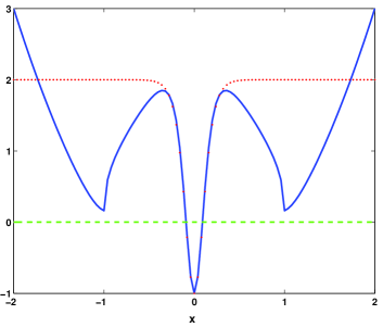
Figure 1: Potentials of operators $L_{\varepsilon}$ (solid line) and $L_{0}$ (dots) for the first excited state.

Step 3: Bounds on the inhomogeneous and nonlinear terms. By symmetries, we note that

$$\hat{H}_{\varepsilon}\in L^{2}_{\rm odd}(\mathbb{R})\quad\mbox{\rm and}\quad\hat{N}_{\varepsilon}(\hat{w}_{\varepsilon}):H^{2}_{\rm odd}(\mathbb{R})\mapsto L^{2}_{\rm odd}(\mathbb{R}).$$

We will show that for small $\varepsilon>0$ and fixed $\alpha\in(0,2)$ there is $C>0$ such that

$$\|\hat{H}_{\varepsilon}\|_{L^{2}\cap L^{\infty}_{\alpha}}\leqslant C\varepsilon^{2/3}.$$ (15)

Using the triangle inequality, we obtain

$$\|\hat{H}_{\varepsilon}\|_{L^{2}}\leqslant\|\eta_{\varepsilon}\|_{L^{\infty}}\|(1-\hat{\eta}^{2}_{\varepsilon}){\rm sech}^{2}(\cdot)\|_{L^{2}}+\sqrt{2}\varepsilon\|\eta_{\varepsilon}^{\prime}\|_{L^{\infty}}\|{\rm sech}^{2}(\cdot)\|_{L^{2}}.$$

By properties (P1) and (P2), for small $\varepsilon>0$ and fixed $\alpha\in(0,2)$ the first term is estimated by

$$\|(1-\hat{\eta}^{2}_{\varepsilon}){\rm sech}^{2}(\cdot)\|_{L^{2}} \leqslant \|(1-\hat{\eta}^{2}_{\varepsilon}){\rm sech}^{2}(\cdot)\|_{L^{2}(|z|\leqslant\varepsilon^{-1/3})}+\|(1-\hat{\eta}^{2}_{\varepsilon}){\rm sech}^{2}(\cdot)\|_{L^{2}(|z|\geqslant\varepsilon^{-1/3})}$$

$$\leqslant \|1-\eta_{\varepsilon}^{2}\|_{L^{\infty}(|x|<\sqrt{2}\varepsilon^{2/3})}\|{\rm sech}^{2}(\cdot)\|_{L^{2}}+\alpha^{-1/2}e^{-\alpha\varepsilon^{-1/3}}\|{\rm sech}^{2}(\cdot)\|_{L^{\infty}_{\alpha}}$$

$$\leqslant C\varepsilon^{4/3}.$$

By property (P3), the second term is estimated by $C\varepsilon^{2/3}$. As a result, for any small $\varepsilon>0$ there is $C>0$ such that $\|\hat{H}_{\varepsilon}\|_{L^{2}}\leqslant C\varepsilon^{2/3}$. By similar arguments, $\hat{H}_{\varepsilon}\in L^{\infty}_{\alpha}(\mathbb{R})$ for any $\alpha\in(0,2)$ and there is $C>0$ such that $\|\hat{H}_{\varepsilon}\|_{L^{\infty}_{\alpha}}\leqslant C\varepsilon^{2/3}$.

To deal with the nonlinear terms, we recall that $H^{2}(\mathbb{R})$ is Banach algebra with respect to multiplication in the sense that

$$\forall\hat{u},\hat{v}\in H^{2}(\mathbb{R}):\quad\|\hat{u}\hat{v}\|_{H^{2}}\leqslant\|\hat{u}\|_{H^{2}}\|\hat{v}\|_{H^{2}}$$

For any $\hat{w}_{\varepsilon}\in H^{2}(\mathbb{R})$, we have

$$\|\hat{N}_{\varepsilon}(\hat{w}_{\varepsilon})\|_{L^{2}}\leqslant 3\|\eta_{\varepsilon}\|_{L^{\infty}}\|\hat{w}_{\varepsilon}^{2}\|_{H^{2}}+\|\hat{w}_{\varepsilon}^{3}\|_{H^{2}}\leqslant 3\|\hat{w}_{\varepsilon}\|^{2}_{H^{2}}+\|\hat{w}_{\varepsilon}\|^{3}_{H^{2}}.$$ (16)

Similarly, $L^{\infty}_{\alpha}(\mathbb{R})$ is a Banach algebra with respect to multiplication for any $\alpha\geqslant 0$.

Step 4: Normal-form transformations. Because we are going to lose $\varepsilon^{2/3}$ as a result of bound (14), we need to perform transformations of solution $\hat{w}_{\varepsilon}$, usually referred to as the normal-form transformations. We need two normal-form transformations to ensure that the resulting operator of a fixed-point equation is a contraction.

Let

$$\hat{w}_{\varepsilon}=\hat{w}_{1}+\hat{w}_{2}+\hat{\varphi}_{\varepsilon},\quad\hat{w}_{1}=\hat{L}_{0}^{-1}\hat{H}_{\varepsilon},\quad\hat{w}_{2}=-3\hat{L}_{0}^{-1}\hat{\eta}_{\varepsilon}\tanh(z)\hat{w}_{1}^{2}.$$

The remainder term $\hat{\varphi}_{\varepsilon}$ solves the new problem

$${\cal L}_{\varepsilon}\hat{\varphi}_{\varepsilon}={\cal H}_{\varepsilon}+{\cal N}_{\varepsilon}(\hat{\varphi}_{\varepsilon}),$$ (17)

where the new linear operator is

$${\cal L}_{\varepsilon}:=\hat{L}_{\varepsilon}+\Delta\hat{U}_{\varepsilon}(z),\quad\Delta\hat{U}_{\varepsilon}(z):=6\hat{\eta}_{\varepsilon}\tanh(z)(\hat{w}_{1}+\hat{w}_{2})+3(\hat{w}_{1}+\hat{w}_{2})^{2},$$

the new source term is

$${\cal H}_{\varepsilon}:=-\hat{U}_{\varepsilon}(\hat{w}_{1}+\hat{w}_{2})-3\hat{\eta}_{\varepsilon}\tanh(z)(2\hat{w}_{1}\hat{w}_{2}+\hat{w}_{2}^{2})-(\hat{w}_{1}+\hat{w}_{2})^{3},$$

and the new nonlinear function is

$${\cal N}_{\varepsilon}(\hat{\varphi}_{\varepsilon}):=-3\hat{\eta}_{\varepsilon}\tanh(z)\hat{\varphi}^{2}_{\varepsilon}-3(\hat{w}_{1}+\hat{w}_{2})\hat{\varphi}_{\varepsilon}^{2}-\hat{\varphi}_{\varepsilon}^{3}.$$

Thanks to bounds (12), (13), and (15), we have $\hat{w}_{1},\hat{w}_{2}\in H^{2}_{\rm odd}(\mathbb{R})\cap L^{\infty}_{\alpha}(\mathbb{R})$ for fixed $\alpha\in(0,2)$ and

$$\exists C>0:\quad\|\hat{w}_{1}\|_{H^{2}\cap L^{\infty}_{\alpha}}\leqslant C\varepsilon^{2/3},\quad\|\hat{w}_{2}\|_{H^{2}\cap L^{\infty}_{\alpha}}\leqslant C\varepsilon^{4/3}.$$ (18)

As a result, for any small $\varepsilon>0$, there is $C>0$ such that

$$\|\hat{\eta}_{\varepsilon}\tanh(z)(2\hat{w}_{1}\hat{w}_{2}+\hat{w}_{2}^{2})\|_{L^{2}}\leqslant C\varepsilon^{2},\quad\|(\hat{w}_{1}+\hat{w}_{2})^{3}\|_{L^{2}}\leqslant C\varepsilon^{2}.$$

Let us now estimate the term $\hat{U}_{\varepsilon}(\hat{w}_{1}+\hat{w}_{2})$ in $L^{2}(\mathbb{R})$. By properties (P1) and (P2), for small $\varepsilon>0$ and fixed $\alpha\in(0,2)$ there are constants $C(\alpha),\tilde{C}(\alpha)>0$ such that

$$\|\hat{U}_{\varepsilon}\hat{w}_{j}\|_{L^{2}} \leqslant 2\varepsilon^{2}\|z^{2}\hat{w}_{j}\|_{L^{2}}+3\|(\hat{\eta}_{\varepsilon}^{2}-1)\hat{w}_{j}\|_{L^{2}}$$

$$\leqslant \varepsilon^{2}C(\alpha)\|\hat{w}_{j}\|_{L^{\infty}_{\alpha}}+3\|(1-\hat{\eta}^{2}_{\varepsilon})\hat{w}_{j}\|_{L^{2}(|z|\leqslant\varepsilon^{-1/3})}+3\|(1-\hat{\eta}^{2}_{\varepsilon})\hat{w}_{j}\|_{L^{2}(|z|\geqslant\varepsilon^{-1/3})}$$

$$\leqslant \varepsilon^{2}C(\alpha)\|\hat{w}_{j}\|_{L^{\infty}_{\alpha}}+3\|1-\eta_{\varepsilon}^{2}\|_{L^{\infty}(|x|<\sqrt{2}\varepsilon^{2/3})}\|\hat{w}_{j}\|_{L^{2}}+3\alpha^{-1/2}e^{-\alpha\varepsilon^{-1/3}}\|\hat{w}_{j}\|_{L^{\infty}_{\alpha}}$$

$$\leqslant \tilde{C}(\alpha)\varepsilon^{4/3}\|\hat{w}_{j}\|_{L^{2}\cap L^{\infty}_{\alpha}},\quad j=1,2.$$

In view of bound (18), for any small $\varepsilon>0$ there is $C>0$ such that

$$\|\hat{U}_{\varepsilon}(\hat{w}_{1}+\hat{w}_{2})\|_{L^{2}}\leqslant C\varepsilon^{2}.$$ (19)

Combining all together, we have established that ${\cal H}_{\varepsilon}\in L^{2}_{\rm odd}(\mathbb{R})$ and for any small $\varepsilon>0$, there is $C>0$ such that

$$\|{\cal H}_{\varepsilon}\|_{L^{2}}\leqslant C\varepsilon^{2}.$$ (20)

For the nonlinear term, we still have ${\cal N}_{\varepsilon}(\hat{\varphi}_{\varepsilon}):H^{2}_{\rm odd}(\mathbb{R})\mapsto L^{2}_{\rm odd}(\mathbb{R})$. Thanks to bound (18), for any $\hat{\varphi}_{\varepsilon}\in B_{\delta}(H^{2}_{\rm odd})$ in the ball of radius $\delta>0$, for any small $\varepsilon>0$ there is $C(\delta)>0$ such that

$$\|{\cal N}_{\varepsilon}(\hat{\varphi}_{\varepsilon})\|_{L^{2}}\leqslant C(\delta)\|\hat{\varphi}_{\varepsilon}\|_{H^{2}}^{2}.$$ (21)

Similarly, we obtain that ${\cal N}_{\varepsilon}$ is Lipschitz continuous in the ball $B_{\delta}(H^{2}_{\rm odd})$ and for any small $\varepsilon>0$ there is $C(\delta)>0$ such that

$$\forall\hat{\varphi}_{\varepsilon},\hat{\varphi}_{\varepsilon}\in B_{\delta}(H^{2}_{\rm odd}):\quad\|{\cal N}_{\varepsilon}(\hat{\varphi}_{\varepsilon})-{\cal N}_{\varepsilon}(\hat{\varphi}_{\varepsilon})\|_{L^{2}}\leqslant C(\delta)\left(\|\hat{\varphi}_{\varepsilon}\|_{H^{2}}+\|\hat{\varphi}_{\varepsilon}\|_{H^{2}}\right)\|\hat{\varphi}_{\varepsilon}-\hat{\varphi}\|_{H^{2}}.$$ (22)

Step 5: Fixed-point arguments. Thanks to bound (18) and Sobolev embedding of $H^{2}(\mathbb{R})$ to $L^{\infty}(\mathbb{R})$, $|\Delta\hat{U}_{\varepsilon}(z)|$ is as small as ${\cal O}(\varepsilon^{2/3})$ in the central well near $z=0$ and is exponentially small in $\varepsilon$ in the two wells near $z=\pm\frac{1}{\sqrt{2}\varepsilon}$. As a result, small positive eigenvalues of $\hat{L}_{\varepsilon}$ of the size ${\cal O}(\varepsilon^{2/3})$ persist in the spectrum of ${\cal L}_{\varepsilon}$ and have the same size, so that bound (14) extends to operator ${\cal L}_{\varepsilon}$ in the form

$$\exists C>0:\quad\forall\hat{f}\in L^{2}_{\rm odd}(\mathbb{R}):\quad\|{\cal L}_{\varepsilon}^{-1}\hat{f}\|_{H^{2}}\leqslant C\varepsilon^{-2/3}\|\hat{f}\|_{L^{2}}.$$ (23)

Let us rewrite equation (17) as the fixed-point problem

$$\hat{\varphi}_{\varepsilon}\in H^{2}_{\rm odd}(\mathbb{R}):\quad\hat{\varphi}_{\varepsilon}={\cal L}_{\varepsilon}^{-1}{\cal H}_{\varepsilon}+{\cal L}_{\varepsilon}^{-1}{\cal N}_{\varepsilon}(\hat{\varphi}_{\varepsilon}).$$ (24)

The map $\hat{\varphi}_{\varepsilon}\mapsto{\cal L}_{\varepsilon}^{-1}{\cal N}_{\varepsilon}(\hat{\varphi}_{\varepsilon})$ is Lipschitz continuous in the neighborhood of $0\in H^{2}_{\rm odd}(\mathbb{R})$. Thanks to bounds (21) and (23), the map is a contraction in the ball $B_{\delta}(H^{2}_{\rm odd})$ if $\delta\ll\varepsilon^{2/3}$. On the other hand, thanks to bounds (20) and (23), the source term ${\cal L}_{\varepsilon}^{-1}{\cal H}_{\varepsilon}$ is as small as ${\cal O}(\varepsilon^{4/3})$ in $L^{2}$ norm. By Banach’s Fixed-Point Theorem in the ball $B_{\delta}(H^{2}_{\rm odd})$ with $\delta\sim\varepsilon^{4/3}$, there exists a unique $\hat{\varphi}_{\varepsilon}\in H^{2}_{\rm odd}(\mathbb{R})$ of the fixed-point problem (24) such that

$$\exists C>0:\quad\|\hat{\varphi}_{\varepsilon}\|_{H^{2}}\leqslant C\varepsilon^{4/3}.$$

By Sobolev’s embedding of $H^{2}(\mathbb{R})$ to ${\cal C}^{1}(\mathbb{R})$, for any small $\varepsilon>0$ there is $C>0$ such that

$$\|w_{\varepsilon}\|_{L^{\infty}}=\|\hat{w}_{\varepsilon}\|_{L^{\infty}}\leqslant C\|\hat{w}_{1}+\hat{w}_{2}+\hat{\varphi}_{\varepsilon}\|_{H^{2}}\leqslant C\varepsilon^{2/3},$$

which completes the proof of bound (10).

Step 6: Properties (9). Solution $\hat{w}_{\varepsilon}$ constructed in Step (5) is a odd continuously differentiable function of $z$ on $\mathbb{R}$ vanishing at infinity, so that $u_{\varepsilon}(0)=0$ and $\lim_{x\to\infty}u_{\varepsilon}(x)=0$. By bootstrapping arguments for the stationary equation (8), we have $u_{\varepsilon}\in{\cal C}^{\infty}(\mathbb{R})$. It remains to prove that $u_{\varepsilon}(x)$ is positive for all $x\in\mathbb{R}_{+}$.

Recall that $\eta_{\varepsilon}(x)>0$ for all $x\in\mathbb{R}$. By property (P4) and bound (10), there is $C>0$ such that $u_{\varepsilon}(x)\geqslant C\varepsilon^{1/3}$ for all $x\in[1,\sqrt{1+\varepsilon^{2/3}}]$. We shall prove that $u_{\varepsilon}(x)>0$ for all $x\geqslant\sqrt{1+\varepsilon^{2/3}}$. Assume by contradiction that there is $x_{0}>\sqrt{1+\varepsilon^{2/3}}$ such that $u_{\varepsilon}(x_{0})=0$ and $u_{\varepsilon}^{\prime}(x_{0})<0$. (If $u_{\varepsilon}^{\prime}(x_{0})=0$, then $u_{\varepsilon}(x)=0$ is the only solution of the second-order equation (8).) The continuity of $u_{\varepsilon}(x)$ implies that $u_{\varepsilon}(x)<0$ for every $x\in(x_{0},\tilde{x}_{0})$ for some $\tilde{x}_{0}>x_{0}$. Using the differential equation (8), we obtain

$$u_{\varepsilon}^{\prime\prime}(x)=\frac{1}{\varepsilon^{2}}(x^{2}-1+u^{2}_{\varepsilon}(x))u_{\varepsilon}(x)<0,\quad x\in(x_{0},\tilde{x}_{0}).$$

Then, $u_{\varepsilon}^{\prime}(x)\leqslant u_{\varepsilon}^{\prime}(x_{0})<0$, so that $u_{\varepsilon}(x)$ is a negative, decreasing function of $x$ for all $x>x_{0}$ with $\tilde{x}_{0}=\infty$. This fact is a contradiction with the decay of $u_{\varepsilon}(x)$ to zero as $x\to\infty$. Therefore, $u_{\varepsilon}(x)>0$ for all $x\in\mathbb{R}_{+}$.

Combining results in Steps (5) and (6), we conclude that $u_{\varepsilon}(x)$ is the first excited state of the stationary equation (8) that satisfies properties (9).

3 Second excited state

The second excited state is an even solution of the stationary equation (8) such that

$$u_{\varepsilon}(x)>0\;\;\mbox{\rm for all}\;\;|x|>x_{0},\quad u_{\varepsilon}(x)<0\;\;\mbox{\rm for all}\;\;|x|<x_{0},\quad\mbox{\rm and}\quad\lim_{x\to\infty}u_{\varepsilon}(x)=0.$$ (25)

Here $x_{0}>0$ determines a location of two symmetric zeros of $u_{\varepsilon}(x)$ at $x=\pm x_{0}$. The second excited state is approximated as $\varepsilon\to 0$ by a product of two copies of dark solitons (Remark 1) placed at $x=\pm a$ with $a\approx x_{0}$ as $\varepsilon\to 0$. Our analysis is based on the method of Lyapunov–Schmidt reductions, which gives existence and convergence properties for the second excited state, as well as an analytical expansion of $a$ for small $\varepsilon$.

Theorem 2

For sufficiently small $\varepsilon>0$, there exists a unique solution $u_{\varepsilon}\in{\cal C}^{\infty}(\mathbb{R})$ with properties (25) and there exist $a>0$ and $C>0$ such that

$$\left\|u_{\varepsilon}-\eta_{\varepsilon}\tanh\left(\frac{\cdot-a}{\sqrt{2}\varepsilon}\right)\tanh\left(\frac{\cdot+a}{\sqrt{2}\varepsilon}\right)\right\|_{L^{\infty}}\leqslant C\varepsilon^{2/3}$$ (26)

and

$$a=-\frac{\varepsilon}{\sqrt{2}}\left(\log(\varepsilon)+\frac{1}{2}\log|\log(\varepsilon)|-\frac{3}{2}\log(2)+o(1)\right)\quad\mbox{\rm as}\quad\varepsilon\to 0.$$ (27)

Remark 2

Since $a\to 0$ as $\varepsilon\to 0$ while $\eta_{\varepsilon}(x)\approx 1$ near $x=0$, we have

$$x_{0}=a+{\cal O}(\varepsilon^{5/3})\quad\mbox{\rm as}\quad\varepsilon\to 0.$$

Remark 3

Exactly the same asymptotic expansion (27) has been obtained with the use of the averaged Lagrangian approximation and has been confirmed numerically [1].

The proof of Theorem 27 follows the same steps as the proof of Theorem 1 with an additional step on the Lyapunov–Schmidt bifurcation equation.

Step 1: Decomposition. Let $a\in(0,1)$ and substitute

$$u_{\varepsilon}(x)=\eta_{\varepsilon}(x)\tanh\left(\frac{x-a}{\sqrt{2}\varepsilon}\right)\tanh\left(\frac{x+a}{\sqrt{2}\varepsilon}\right)+w_{\varepsilon}(x)$$

to the stationary equation (8). The equivalent problem for $w_{\varepsilon}$ takes the operator form

$$L_{\varepsilon}w_{\varepsilon}=H_{\varepsilon}+N_{\varepsilon}(w_{\varepsilon}),$$ (28)

where

$$L_{\varepsilon}:=-\varepsilon^{2}\partial_{x}^{2}+x^{2}-1+3\eta_{\varepsilon}^{2}(x)\tanh^{2}(z_{+})\tanh^{2}(z_{-}),$$

$$H_{\varepsilon} := \eta_{\varepsilon}(x)(\eta_{\varepsilon}^{2}(x)-1)\tanh(z_{+})\tanh(z_{-})\left({\rm sech}^{2}(z_{+})+{\rm sech}^{2}(z_{-})\right)$$

$$+\eta_{\varepsilon}(x){\rm sech}^{2}(z_{+}){\rm sech}^{2}(z_{-})\left(1-\eta_{\varepsilon}^{2}(x)\tanh(z_{+})\tanh(z_{-})\right)$$

$$+\sqrt{2}\varepsilon\eta_{\varepsilon}^{\prime}(x)\left(\tanh(z_{+}){\rm sech}^{2}(z_{-})+\tanh(z_{-}){\rm sech}^{2}(z_{+})\right),$$

and

$$N_{\varepsilon}(w_{\varepsilon})=-3\eta_{\varepsilon}(x)\tanh(z_{+})\tanh(z_{-})w_{\varepsilon}^{2}(x)-w_{\varepsilon}^{3}(x),$$

with the following notations

$$z_{\pm}=z\pm\zeta,\quad z=\frac{x}{\sqrt{2}\varepsilon},\quad\zeta=\frac{a}{\sqrt{2}\varepsilon}.$$

We again denote the functions in $z$ by hats. We shall assume a priori that

$$\left\{\begin{array}[]{l}\exists\beta\in(0,1):\quad a\leqslant\sqrt{2}\beta\varepsilon^{2/3},\\ \exists C>0:\quad e^{-2\zeta}\leqslant C\varepsilon|\log(\varepsilon)|^{1/2}.\end{array}\right.$$ (29)

Note that bounds (29) imply that $a\to 0$ and $\zeta\to\infty$ as $\varepsilon\to 0$.

Step 2: Linear estimates. In new variables, operator $L_{\varepsilon}$ becomes

$$\hat{L}_{\varepsilon}=-\frac{1}{2}\partial_{z}^{2}+2\varepsilon^{2}z^{2}-1+3\hat{\eta}_{\varepsilon}^{2}(z)\tanh^{2}(z+\zeta)\tanh^{2}(z-\zeta)\equiv\hat{L}_{0}(\zeta)+\hat{U}_{\varepsilon}(z,\zeta),$$

where

$$\hat{L}_{0}(\zeta)=-\frac{1}{2}\partial_{z}^{2}+2-3{\rm sech}^{2}(z+\zeta)-3{\rm sech}^{2}(z-\zeta)$$

and

$$\hat{U}_{\varepsilon}(z,\zeta)=2\varepsilon^{2}z^{2}+3(\hat{\eta}^{2}_{\varepsilon}(z)-1)\tanh^{2}(z+\zeta)\tanh^{2}(z-\zeta)+3{\rm sech}^{2}(z+\zeta){\rm sech}^{2}(z-\zeta).$$

Operator $\hat{L}_{0}(\zeta)$ has now two eigenvalues in the neighborhood of $0$ for large $\zeta$ because of the double-well potential centered at $z=\pm\zeta$. If $\zeta$ is large, the geometric splitting theory [10] implies that the eigenfunctions $\hat{\psi}^{\pm}_{0}(z)$ of operator $\hat{L}_{0}(\zeta)$ corresponding to the two smallest eigenvalues are given asymptotically by

$$\hat{\psi}^{\pm}_{0}(z)=\frac{\hat{\psi}_{0}(z-\zeta)\pm\hat{\psi}_{0}(z+\zeta)}{\sqrt{2}}+{\cal O}_{L^{\infty}}(e^{-2\zeta})\quad\mbox{\rm as}\quad\zeta\to\infty,$$ (30)

where $\hat{\psi}_{0}(z)=\frac{\sqrt{3}}{2}{\rm sech}^{2}(z)$ is the $L^{2}$-normalized eigenfunction of $\hat{L}_{0}=-\frac{1}{2}\partial_{z}^{2}+2-3{\rm sech}^{2}(z)$ for the zero eigenvalue.

Note that $\hat{\psi}^{+}_{0}(z)$ is even and $\hat{\psi}^{-}_{0}(z)$ is odd on $\mathbb{R}$. For the second excited state, we are looking for an even solution $\hat{w}_{\varepsilon}(z)$. Since $a$ is not specified yet, we add the condition $\langle\hat{\psi}^{+}_{0},\hat{w}_{\varepsilon}\rangle=0$ and define a constrained subspace of $H^{2}_{\rm even}(\mathbb{R})$ by

$$X_{0}=\{\hat{w}_{\varepsilon}\in H^{2}_{\rm even}(\mathbb{R}):\quad\langle\hat{\psi}^{+}_{0},\hat{w}_{\varepsilon}\rangle=0\}.$$

Let $P_{0}$ be an orthogonal projection operator to the complement of $\hat{\psi}^{+}_{0}$ in $L^{2}_{\rm even}(\mathbb{R})$. Since eigenfunction $\hat{\psi}^{-}_{0}$ is odd and the rest of spectrum of $\hat{L}_{0}(\zeta)$ is bounded from zero, for any $\hat{f}\in L^{2}_{\rm even}(\mathbb{R})$, there exists a unique $P_{0}\hat{L}^{-1}_{0}(\zeta)P_{0}\hat{f}\in H^{2}_{\rm even}(\mathbb{R})$ such that

$$\exists C>0:\quad\forall\hat{f}\in L^{2}_{\rm even}(\mathbb{R}):\quad\|P_{0}\hat{L}^{-1}_{0}(\zeta)P_{0}\hat{f}\|_{H^{2}}\leqslant C\|\hat{f}\|_{L^{2}}.$$ (31)

Let us consider functions that decay to zero as $|z-\zeta|,|z+\zeta|\to\infty$ with a fixed exponential decay rate $\alpha>0$. Let $L^{\infty}_{\alpha,\zeta}(\mathbb{R})$ be the exponentially weighted space with the supremum norm

$$\|\hat{w}_{\varepsilon}\|_{L^{\infty}_{\alpha,\zeta}}:=\sup_{z\in\mathbb{R}_{+}}e^{\alpha(|z-\zeta|)}|\hat{w}_{\varepsilon}(z)|+\sup_{z\in\mathbb{R}_{-}}e^{\alpha(|z+\zeta|)}|\hat{w}_{\varepsilon}(z)|.$$

For fixed $\alpha>0$ and $\zeta>0$, the unique solution $P_{0}\hat{L}^{-1}_{0}(\zeta)P_{0}\hat{f}$ decays exponentially with the same rate as $\hat{f}$ so that

$$\exists C>0:\quad\forall\hat{f}\in L^{2}_{\rm even}(\mathbb{R})\cap L^{\infty}_{\alpha}(\mathbb{R}):\quad\|P_{0}\hat{L}^{-1}_{0}(\zeta)P_{0}\hat{f}\|_{L^{\infty}_{\alpha,\zeta}}\leqslant C\|\hat{f}\|_{L^{\infty}_{\alpha,\zeta}}.$$ (32)

Figure 2 shows the potential $V_{\varepsilon}(x)=x^{2}-1+3\eta_{\varepsilon}^{2}(x)\tanh^{2}(z+\zeta)\tanh^{2}(z-\zeta)$ of operator $L_{\varepsilon}=-\varepsilon^{2}\partial_{x}^{2}+V_{\varepsilon}(x)$ (solid line) and the potential $V_{0}(x)=2-3{\rm sech}^{2}(z+\zeta)-3{\rm sech}^{2}(z-\zeta)$ of operator $L_{0}=-\varepsilon^{2}\partial_{x}^{2}+V_{0}(x)$ (dots) versus $x$. The bounded potential $V_{0}(x)$ has two wells near $x=\pm a$, whereas the confining potential $V_{\varepsilon}(x)$ has four wells near $x=\pm a$ and $x=\pm 1$.

Again, the spectrum of operator $\hat{L}_{\varepsilon}$ with a confining potential is purely discrete. The two wells of the confining potential $V_{\varepsilon}(x)$ near $x=\pm 1$ are ${\cal O}(\varepsilon^{2/3})$-close to zero but still positive thanks to property (P4) and the fact that $\tanh(z\pm\zeta)=1$ with exponential accuracy in $\varepsilon$ if $\zeta\leqslant\beta\varepsilon^{-1/3}$ for fixed $\beta\in(0,1)$. Therefore, for any fixed $x_{0}>0$, we have

$$\exists C>0:\quad V(x)\geqslant C\varepsilon^{2/3},\quad|x|\geqslant x_{0}.$$ (33)

On the other hand, by property (P2) for any $\zeta\in(0,\varepsilon^{-2/3})$, we have

$$\exists C>0:\quad\sup_{|z|\leqslant\varepsilon^{-2/3}}|\hat{U}_{\varepsilon}(z,\zeta)|\leqslant C(\varepsilon^{2/3}+e^{-4\zeta}).$$ (34)

Thanks to properties (33) and (34), the quantum tunneling theory [5] implies that the two small eigenvalues of $\hat{L}_{0}$ persist as two small eigenvalues of $\hat{L}_{\varepsilon}$ with two eigenfunctions $\hat{\psi}^{\pm}_{\varepsilon}$ that satisfy asymptotically

$$\hat{\psi}^{\pm}_{\varepsilon}(z)=\hat{\psi}^{\pm}_{0}(z)+{\cal O}_{L^{\infty}}(\varepsilon^{2/3})\quad\mbox{\rm as}\quad\varepsilon\to 0,$$ (35)

thanks to a priori bound (29) and the exponential smallness of $\hat{\psi}^{\pm}_{0}(z)$ in $\varepsilon$ near $z=\pm\frac{1}{\sqrt{2}\varepsilon}$.

Let $P_{\varepsilon}$ be an orthogonal projection operator to the complement of $\hat{\psi}^{+}_{\varepsilon}$ in $L^{2}_{\rm even}(\mathbb{R})$. Because of the small ${\cal O}(\varepsilon^{2/3})$ eigenvalues of $\hat{L}_{\varepsilon}$, bound (31) is now replaced by

$$\exists C>0:\quad\forall\hat{f}\in L^{2}_{\rm even}(\mathbb{R}):\quad\|P_{\varepsilon}\hat{L}_{\varepsilon}^{-1}P_{\varepsilon}\hat{f}\|_{H^{2}}\leqslant C\varepsilon^{-2/3}\|\hat{f}\|_{L^{2}}.$$ (36)

The function $P_{\varepsilon}\hat{L}_{\varepsilon}^{-1}P_{\varepsilon}\hat{f}\in H^{2}_{\rm even}(\mathbb{R})$ has peaks in all four wells near points $z=\pm\frac{1}{\sqrt{2}\varepsilon}$ and $z=\pm\zeta$.

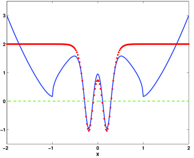
Figure 2: Potential of operator $L_{\varepsilon}$ (solid line) and $L_{0}$ (dots) for the second excited state.

Step 3: Bounds on the inhomogeneous and nonlinear terms. From the symmetry of terms in $\hat{H}_{\varepsilon}$ and $\hat{N}_{\varepsilon}(\hat{w}_{\varepsilon})$, we have

$$\hat{N}_{\varepsilon}(\hat{w}_{\varepsilon}):H^{2}_{\rm even}(\mathbb{R})\mapsto L^{2}_{\rm even}(\mathbb{R})\quad{\rm and}\quad\hat{H}_{\varepsilon}\in L^{2}_{\rm even}(\mathbb{R}).$$

Under a priori bound (29), we first show that there is $C>0$ such that

$$\|\hat{H}_{\varepsilon}\|_{L^{2}} \leqslant C\varepsilon^{2/3}.$$ (37)

The upper bound for the first term in $\hat{H}_{\varepsilon}$ involves estimates of

$$I_{1}(z):=(1-\hat{\eta}^{2}_{\varepsilon}(z))({\rm sech}^{2}(z+\zeta)+{\rm sech}^{2}(z-\zeta)),$$

which may create a problem since $\zeta\to\infty$ as $\varepsilon\to 0$ and $\hat{\eta}_{\varepsilon}(z)\to 0$ as $|z|\to\infty$. By properties (P1) and (P2), for any $\alpha\in(0,2)$, $\zeta\leqslant\beta\varepsilon^{-1/3}$ for any $\beta\in(0,1)$, and any small $\varepsilon>0$, there is constant $C>0$ such that

$$\|I_{1}\|_{L^{2}} \leqslant \|I_{1}\|_{L^{2}(|z|\leqslant\varepsilon^{-1/3})}+\|I_{1}\|_{L^{2}(|z|\geqslant\varepsilon^{-1/3})}$$

$$\leqslant \|1-\eta_{\varepsilon}^{2}\|_{L^{\infty}(|x|<\sqrt{2}\varepsilon^{2/3})}\|{\rm sech}^{2}(z_{+})+{\rm sech}^{2}(z_{-})\|_{L^{2}}$$

$$\phantom{texttext}+\alpha^{-1/2}e^{-\alpha(\varepsilon^{-1/3}-\zeta)}\|{\rm sech}^{2}(z_{+})+{\rm sech}^{2}(z_{-})\|_{L^{\infty}_{\alpha,\zeta}}$$

$$\leqslant C\varepsilon^{4/3}.$$

Thus, the condition $\zeta\leqslant\beta\varepsilon^{-1/3}$ from a priori bound (29) is sufficient to keep $I_{1}$ small in $L^{2}$.

The upper bound for the second term in $\hat{H}_{\varepsilon}$ involves the estimate of the overlapping term

$$I_{2}(z):={\rm sech}^{2}(z_{+}){\rm sech}^{2}(z_{-}).$$

Under a priori bound (29), this term is estimated by

$$\|I_{2}\|_{L^{2}} \leqslant \left(\int_{\mathbb{R}}{\rm sech}^{4}(z+\zeta){\rm sech}^{4}(z-\zeta)dz\right)^{1/2}$$

$$= \left(2\int_{-\zeta}^{\infty}{\rm sech}^{4}(u){\rm sech}^{4}(u+2\zeta)du\right)^{1/2}\leqslant Ce^{-2\zeta}\leqslant C\varepsilon|\log(\varepsilon)|^{1/2}.$$

The last term in $\hat{H}_{\varepsilon}$ is proportional to $\varepsilon\eta_{\varepsilon}^{\prime}$ and is handled with property (P3) to give (37). By similar arguments, $\hat{H}_{\varepsilon}\in L^{\infty}_{\alpha,\zeta}(\mathbb{R})$ for any $\alpha\in(0,2)$ and $\zeta\leqslant\beta\varepsilon^{-1/3}$ for any $\beta\in(0,1)$ and for any small $\varepsilon>0$ there is $C>0$ such that $\|\hat{H}_{\varepsilon}\|_{L^{\infty}_{\alpha,\zeta}}\leqslant C\varepsilon^{2/3}$.

The nonlinear terms in $\hat{N}_{\varepsilon}(\hat{w}_{\varepsilon})$ are handled with the Banach algebra of $H^{2}(\mathbb{R})$, so we obtain

$$\|\hat{N}_{\varepsilon}(\hat{w}_{\varepsilon})\|_{L^{2}}\leqslant 3\|\hat{w}_{\varepsilon}\|^{2}_{H^{2}}+\|\hat{w}_{\varepsilon}\|^{3}_{H^{2}}.$$ (38)

Step 4: Normal-form transformations. Unlike step (4) in the proof of Theorem 1, we need to perform a sequence of two normal-form transformations because the orthogonal projection operator to the one-dimensional subspace spanned by an even eigenfunction for the smallest eigenvalue of $\hat{L}_{0}$ has to be changed to the projection operator associated with an eigenfunction of a new linearization operator. For the sake of short notations, we combine both normal-form transformations and write them together.

Let $\hat{w}_{\varepsilon}=\hat{w}_{1}+\hat{w}_{2}+\hat{\varphi}_{\varepsilon}$ with

$$\hat{w}_{1}=P_{0}\hat{L}_{0}^{-1}P_{0}\hat{H}_{\varepsilon},\quad\hat{w}_{2}=P_{0}\hat{L}_{0}^{-1}P_{0}\hat{G}_{\varepsilon},$$

where

$$\hat{G}_{\varepsilon}:=-3\hat{\eta}_{\varepsilon}\tanh(z+\zeta)\tanh(z-\zeta)\hat{w}_{1}^{2}+({\cal P}_{\varepsilon}-P_{0})\hat{H}_{\varepsilon}$$

and ${\cal P}_{\varepsilon}$ is a new orthogonal projection operator introduced below.

The remainder term $\hat{\varphi}_{\varepsilon}$ solves the new problem

$${\cal L}_{\varepsilon}\hat{\varphi}_{\varepsilon}={\cal H}_{\varepsilon}+{\cal N}_{\varepsilon}(\hat{\varphi}_{\varepsilon})+{\cal S}_{\varepsilon},$$ (39)

where the new linear operator is

$${\cal L}_{\varepsilon}:=\hat{L}_{\varepsilon}+\Delta\hat{U}_{\varepsilon}(z),\quad\Delta\hat{U}_{\varepsilon}(z):=6\hat{\eta}_{\varepsilon}\tanh(z+\zeta)\tanh(z-\zeta)(\hat{w}_{1}+\hat{w}_{2})+3(\hat{w}_{1}+\hat{w}_{2})^{2},$$

the new source term is

$${\cal H}_{\varepsilon}:=-\hat{U}_{\varepsilon}(\hat{w}_{1}+\hat{w}_{2})-3\hat{\eta}_{\varepsilon}\tanh(z+\zeta)\tanh(z-\zeta)(2\hat{w}_{1}\hat{w}_{2}+\hat{w}_{2}^{2})-(\hat{w}_{1}+\hat{w}_{2})^{3}+({\cal P}_{\varepsilon}-P_{0})\hat{G}_{\varepsilon},$$

the new nonlinear function is

$${\cal N}_{\varepsilon}(\hat{\varphi}_{\varepsilon}):=-3\hat{\eta}_{\varepsilon}\tanh(z+\zeta)\tanh(z-\zeta)\hat{\varphi}^{2}_{\varepsilon}-3(\hat{w}_{1}+\hat{w}_{2})\hat{\varphi}_{\varepsilon}^{2}-\hat{\varphi}_{\varepsilon}^{3},$$

and the new one-dimensional projection is

$${\cal S}_{\varepsilon}:=(I-{\cal P}_{\varepsilon})(\hat{H}_{\varepsilon}+\hat{G}_{\varepsilon}).$$

If $\hat{w}_{1},\hat{w}_{2}\in H^{2}(\mathbb{R})\cap L^{\infty}_{\alpha,\zeta}(\mathbb{R})$ satisfy bounds (42) below, then $\Delta\hat{U}_{\varepsilon}(z)$ is as small as ${\cal O}(\varepsilon^{2/3})$ in the two wells near $z=\pm\zeta$ and is exponentially small in $\varepsilon$ in the two wells near $z=\pm\frac{1}{\sqrt{2}\varepsilon}$. Let $\tilde{\psi}^{\pm}_{\varepsilon}$ be the eigenfunctions of ${\cal L}_{\varepsilon}$ for the two eigenvalues continued from the two smallest eigenvalues of $\hat{L}_{0}$. The proximity of the potential wells and expansion (35) imply that

$$\tilde{\psi}^{\pm}_{\varepsilon}(z)=\hat{\psi}^{\pm}_{\varepsilon}(z)+{\cal O}_{L^{\infty}}(\varepsilon^{2/3})=\hat{\psi}^{\pm}_{0}(z)+{\cal O}_{L^{\infty}}(\varepsilon^{2/3})\quad\mbox{\rm as}\quad\varepsilon\to 0.$$ (40)

Let ${\cal P}_{\varepsilon}$ be an orthogonal projection operator to the complement of $\tilde{\psi}^{+}_{\varepsilon}$ in $L^{2}_{\rm even}(\mathbb{R})$. Thanks to expansion (40), we have

$$\exists C>0:\quad\|{\cal P}_{\varepsilon}-P_{0}\|_{L^{2}\to L^{2}}\leqslant C\varepsilon^{2/3}.$$ (41)

Thanks to bounds (31), (32), (37), and (41), we have $\hat{w}_{1},\hat{w}_{2}\in H^{2}_{\rm even}(\mathbb{R})\cap L^{\infty}_{\alpha,\zeta}(\mathbb{R})$ for any $\alpha\in(0,2)$ and $\zeta\leqslant\beta\varepsilon^{-1/3}$ for any $\beta\in(0,1)$ such that

$$\exists C>0:\quad\|\hat{w}_{1}\|_{H^{2}\cap L^{\infty}_{\alpha,\zeta}}\leqslant C\varepsilon^{2/3},\quad\|\hat{w}_{2}\|_{H^{2}\cap L^{\infty}_{\alpha,\zeta}}\leqslant C\varepsilon^{4/3}.$$ (42)

As a result, for any small $\varepsilon>0$, there is $C>0$ such that

$$\|\hat{\eta}_{\varepsilon}\tanh(z+\zeta)\tanh(z-\zeta)(2\hat{w}_{1}\hat{w}_{2}+\hat{w}_{2}^{2})\|_{L^{2}} \leqslant C\varepsilon^{2},$$

$$\|(\hat{w}_{1}+\hat{w}_{2})^{3}\|_{L^{2}} \leqslant C\varepsilon^{2},$$

$$\|({\cal P}_{\varepsilon}-P_{0})\hat{G}_{\varepsilon}\|_{L^{2}} \leqslant C\varepsilon^{2}.$$

Let us now estimate the term $\hat{U}_{\varepsilon}\hat{w}_{j}$ in $L^{2}(\mathbb{R})$ for any $j=\{1,2\}$. By properties (P1) and (P2), for any $\alpha\in(0,2)$ and $\zeta\leqslant\beta\varepsilon^{-1/3}$ for any $\beta\in(0,1)$, and for any small $\varepsilon>0$, we have

$$\|\varepsilon^{2}z^{2}\hat{w}_{j}\|_{L^{2}} \leqslant C\varepsilon^{2}\zeta^{2}\|\hat{w}_{j}\|_{L^{\infty}_{\alpha,\zeta}}\leqslant C\varepsilon^{4/3}\|\hat{w}_{j}\|_{L^{\infty}_{\alpha,\zeta}},$$

$$\|(1-\hat{\eta}_{\varepsilon}^{2})\hat{w}_{j}\|_{L^{2}} \leqslant \|(1-\hat{\eta}^{2}_{\varepsilon})\hat{w}_{j}\|_{L^{2}(|z|\leqslant\varepsilon^{-1/3})}+\|(1-\hat{\eta}^{2}_{\varepsilon})\hat{w}_{j}\|_{L^{2}(|z|\geqslant\varepsilon^{-1/3})}$$

$$\leqslant \|1-\eta_{\varepsilon}^{2}\|_{L^{\infty}(|x|<\sqrt{2}\varepsilon^{2/3})}\|\hat{w}_{j}\|_{L^{2}}+\alpha^{-1/2}e^{-\alpha(\varepsilon^{-1/3}-\zeta)}\|\hat{w}_{j}\|_{L^{\infty}_{\alpha,\zeta}}$$

$$\leqslant C\varepsilon^{4/3}\|\hat{w}_{j}\|_{L^{2}\cap L^{\infty}_{\alpha,\zeta}},$$

$$\|{\rm sech}^{2}(z_{+}){\rm sech}^{2}(z_{-})\hat{w}_{\varepsilon}\|_{L^{2}} \leqslant Ce^{-4\zeta}\|\hat{w}_{\varepsilon}\|_{L^{2}}\leqslant C\varepsilon^{2}|\log(\varepsilon)|\|\hat{w}_{\varepsilon}\|_{L^{2}}.$$

In view of bound (42), for any small $\varepsilon>0$, there is $C>0$ such that

$$\|\hat{U}_{\varepsilon}(\hat{w}_{1}+\hat{w}_{2})\|_{L^{2}}\leqslant C\varepsilon^{2}.$$ (43)

Combining all together, we have established that ${\cal H}_{\varepsilon}\in L^{2}_{\rm even}(\mathbb{R})$ and for any small $\varepsilon>0$, there is $C>0$ such that

$$\|{\cal H}_{\varepsilon}\|_{L^{2}}\leqslant C\varepsilon^{2}.$$ (44)

For the nonlinear term, we still have ${\cal N}_{\varepsilon}(\hat{\varphi}_{\varepsilon}):H^{2}_{\rm even}(\mathbb{R})\mapsto L^{2}_{\rm even}(\mathbb{R})$. Thanks to bound (42), for any $\hat{\varphi}_{\varepsilon}\in B_{\delta}(H^{2}_{\rm even})$ in the ball of radius $\delta>0$ and for any small $\varepsilon>0$, there is $C(\delta)>0$ such that

$$\|{\cal N}_{\varepsilon}(\hat{\varphi}_{\varepsilon})\|_{L^{2}}\leqslant C(\delta)\|\hat{\varphi}_{\varepsilon}\|_{H^{2}}^{2}.$$ (45)

Step 5: Fixed-point arguments. Because $\Delta\hat{U}_{\varepsilon}(z)$ is exponentially small in $\varepsilon$ near $z=\pm\frac{1}{\sqrt{2}\varepsilon}$, small positive eigenvalues of $\hat{L}_{\varepsilon}$ of the size ${\cal O}(\varepsilon^{2/3})$ persist in the spectrum of ${\cal L}_{\varepsilon}$ and have the same size. As a result, bound (36) extends to the operator ${\cal L}_{\varepsilon}$ in the form

$$\exists C>0:\quad\forall\hat{f}\in L^{2}_{\rm even}(\mathbb{R}):\quad\|{\cal P}_{\varepsilon}\hat{L}_{\varepsilon}^{-1}{\cal P}_{\varepsilon}\hat{f}\|_{H^{2}}\leqslant C\varepsilon^{-2/3}\|\hat{f}\|_{L^{2}},$$ (46)

where the new projection operator ${\cal P}_{\varepsilon}$ is used. As a result, we rewrite equation (39) as the fixed-point problem

$$\hat{\varphi}_{\varepsilon}\in H^{2}_{\rm even}(\mathbb{R}):\quad\hat{\varphi}_{\varepsilon}={\cal P}_{\varepsilon}{\cal L}_{\varepsilon}^{-1}{\cal P}_{\varepsilon}\left({\cal H}_{\varepsilon}+{\cal N}_{\varepsilon}(\hat{\varphi}_{\varepsilon})+{\cal S}_{\varepsilon}\right).$$ (47)

subject to the Lyapunov–Schmidt bifurcation equation

$${\cal F}_{\varepsilon}:=\langle\tilde{\psi}^{+}_{\varepsilon},({\cal H}_{\varepsilon}+{\cal N}_{\varepsilon}(\hat{\varphi}_{\varepsilon})+{\cal S}_{\varepsilon})\rangle_{L^{2}}=\langle\tilde{\psi}^{+}_{\varepsilon},(\hat{H}_{\varepsilon}+\hat{G}_{\varepsilon}+{\cal H}_{\varepsilon}+{\cal N}_{\varepsilon}(\hat{\varphi}_{\varepsilon}))\rangle_{L^{2}}=0.$$ (48)

The map $\hat{\varphi}_{\varepsilon}\mapsto{\cal P}_{\varepsilon}{\cal L}_{\varepsilon}^{-1}{\cal P}_{\varepsilon}{\cal N}_{\varepsilon}(\hat{\varphi}_{\varepsilon})$ is Lipschitz continuous in the neighborhood of $0\in H^{2}_{\rm even}(\mathbb{R})$. Thanks to bounds (45) and (46), the map is a contraction in the ball $B_{\delta}(H^{2}_{\rm even})$ if $\delta\ll\varepsilon^{2/3}$. On the other hand, thanks to bounds (44) and (46), the source term ${\cal P}_{\varepsilon}{\cal L}_{\varepsilon}^{-1}{\cal P}_{\varepsilon}{\cal H}_{\varepsilon}$ is as small as ${\cal O}(\varepsilon^{4/3})$ in $L^{2}$ norm. Furthermore, ${\cal P}_{\varepsilon}{\cal S}_{\varepsilon}=0$.

By Banach’s Fixed-Point Theorem in the ball $B_{\delta}(H^{2}_{\rm even})$ with $\delta\sim\varepsilon^{4/3}$, for any $(a,\zeta)$ satisfying a priori bounds (29) and sufficiently small $\varepsilon>0$, there exists a unique $\hat{\varphi}_{\varepsilon}\in H^{2}_{\rm even}(\mathbb{R})$ of the fixed-point problem (47) and $C>0$ such that

$$\|\hat{\varphi}_{\varepsilon}\|_{H^{2}}\leqslant C\varepsilon^{4/3}.$$

By Sobolev’s embedding of $H^{2}(\mathbb{R})$ to ${\cal C}^{1}(\mathbb{R})$, for any small $\varepsilon>0$ there is $C>0$ such that

$$\|w_{\varepsilon}\|_{L^{\infty}}=\|\hat{w}_{\varepsilon}\|_{L^{\infty}}\leqslant C\|\hat{w}_{1}+\hat{w}_{2}+\hat{\varphi}_{\varepsilon}\|_{H^{2}}\leqslant C\varepsilon^{2/3},$$

which completes the proof of bound (26) for any $(a,\zeta)$ satisfying a priori bounds (29). It remains to show that bounds (29) are satisfied by solutions of the Lyapunov–Schmidt bifurcation equation (48).

Step 6: Lyapunov–Schmidt bifurcation equation. To consider solutions of the Lyapunov–Schmidt reduction equation, we rewrite (48) in the form

$${\cal F}_{\varepsilon}\equiv{\cal F}_{\varepsilon}^{(1)}+{\cal F}_{\varepsilon}^{(2)},$$

where

$${\cal F}_{\varepsilon}^{(1)} = \langle\hat{\psi}^{+}_{0},\hat{H}_{\varepsilon}\rangle_{L^{2}},$$

$${\cal F}_{\varepsilon}^{(2)} = \langle\tilde{\psi}^{+}_{\varepsilon},\left(\hat{G}_{\varepsilon}+{\cal H}_{\varepsilon}+{\cal N}_{\varepsilon}(\hat{\varphi}_{\varepsilon})\right)\rangle_{L^{2}}+\langle\tilde{\psi}^{+}_{\varepsilon}-\hat{\psi}^{+}_{0},\hat{H}_{\varepsilon}\rangle_{L^{2}}.$$

We will show that there exists a simple root of ${\cal F}_{\varepsilon}^{(1)}$ in $a>0$, which satisfies the asymptotic expansion (27) and that this root persists with respect to the perturbations in ${\cal F}_{\varepsilon}^{(2)}$. If $a$ satisfies the asymptotic expansion (27), then $a={\cal O}(\varepsilon|\log(\varepsilon)|)$ and $e^{-2\zeta}={\cal O}(\varepsilon|\log(\varepsilon)|^{1/2})$ so that a priori bounds (29) are satisfied.

For convenience, we recall (30) and write

$${\cal R}_{\varepsilon}\equiv\frac{2\sqrt{2}}{\sqrt{3}}{\cal F}_{\varepsilon}^{(1)}=\langle({\rm sech}^{2}(z_{+})+{\rm sech}^{2}(z_{-})+{\cal O}_{L^{\infty}}(e^{-2\zeta}),\hat{H}_{\varepsilon}\rangle_{L^{2}}.$$ (49)

In what follows, we compute the leading order of ${\cal R}$ and account the error of the size ${\cal O}_{L^{\infty}}(e^{-2\zeta})$ in the end of computations. From explicit definition of $\hat{H}_{\varepsilon}$, the leading-order part of ${\cal R}_{\varepsilon}$ is written in the form

$${\cal R}_{\varepsilon}^{(1)} = \langle({\rm sech}^{2}(z_{+})+{\rm sech}^{2}(z_{-}),\hat{H}_{\varepsilon}\rangle_{L^{2}}$$

$$= \int_{\mathbb{R}}\eta_{\varepsilon}(x)(\eta_{\varepsilon}^{2}(x)-1)\tanh(z_{+})\tanh(z_{-})\left({\rm sech}^{2}(z_{+})+{\rm sech}^{2}(z_{-})\right)^{2}dz$$

$$+\sqrt{2}\varepsilon\int_{\mathbb{R}}\eta_{\varepsilon}^{\prime}(x)\left(\tanh(z_{+}){\rm sech}^{2}(z_{-})+\tanh(z_{-}){\rm sech}^{2}(z_{+})\right)\left({\rm sech}^{2}(z_{+})+{\rm sech}^{2}(z_{-})\right)dz$$

$$+\int_{\mathbb{R}}\eta_{\varepsilon}(x){\rm sech}^{2}(z_{+}){\rm sech}^{2}(z_{-})\left(1-\eta_{\varepsilon}^{2}(x)\tanh(z_{+})\tanh(z_{-})\right)\left({\rm sech}^{2}(z_{+})+{\rm sech}^{2}(z_{-})\right)dz.$$

After the change of variables $u=z-\zeta=z_{-}=z_{+}-2\zeta$ and the use of symmetry on $z\in\mathbb{R}$, the first and second terms in ${\cal R}_{\varepsilon}$ give

$$I_{1}+I_{2} = 2\int_{-\zeta}^{\infty}\eta_{\varepsilon}(x)(\eta_{\varepsilon}^{2}(x)-1)\tanh(u)\tanh(u+2\zeta)\left({\rm sech}^{2}(u)+{\rm sech}^{2}(u+2\zeta)\right)^{2}du$$

$$+2\sqrt{2}\varepsilon\int_{-\zeta}^{\infty}\eta_{\varepsilon}^{\prime}(x)\left(\tanh(u){\rm sech}^{2}(u+2\zeta)+\tanh(u+2\zeta){\rm sech}^{2}(u)\right)$$

$$\phantom{texttexttexttexttexttexttexttext}\times\left({\rm sech}^{2}(u)+{\rm sech}^{2}(u+2\zeta)\right)du$$

$$= \frac{3\sqrt{2}\varepsilon}{2}\int_{-\zeta}^{\infty}(1+\eta^{2}_{\varepsilon}(x))\eta_{\varepsilon}^{\prime}(x){\rm sech}^{4}(u)\left(1+{\cal O}_{L^{\infty}}(e^{-2\zeta})\right)du$$

where $x=\sqrt{2}\varepsilon(u+\zeta)$. Thanks to the exponential decay of ${\rm sech}^{4}(u)$ and property (P3), we have

$$I_{1}+I_{2}=\frac{3\sqrt{2}\varepsilon}{2}\int_{-\zeta}^{\zeta}(1+\eta^{2}_{\varepsilon}(x))\eta_{\varepsilon}^{\prime}(x){\rm sech}^{4}(u)\left(1+{\cal O}_{L^{\infty}}(e^{-2\zeta})\right)du+{\cal O}(\varepsilon^{2/3}e^{-4\zeta}).$$ (50)

On the other hand, thanks to property (P2) for $\zeta\leqslant\beta\varepsilon^{-1/3}$ for any $\beta\in(0,1)$, we have

$$\eta_{\varepsilon}(x)=1+{\cal O}_{L^{\infty}}(\varepsilon^{4/3}),\quad\eta_{\varepsilon}^{\prime}(x)=-x(1+{\cal O}_{L^{\infty}}(\varepsilon^{4/3})),\quad\forall x\in[0,2\sqrt{2}\varepsilon\zeta].$$

As a result, we obtain

$$I_{1}+I_{2} = -6\varepsilon^{2}\int_{-\zeta}^{\zeta}(\zeta+u){\rm sech}^{4}(u)\left(1+{\cal O}_{L^{\infty}}(\varepsilon^{4/3},e^{-2\zeta})\right)du+{\cal O}(\varepsilon^{2/3}e^{-4\zeta})$$

$$= -4\sqrt{2}\varepsilon a\left(1+{\cal O}(\varepsilon^{4/3},e^{-2\zeta})\right)+{\cal O}(\varepsilon^{2/3}e^{-4\zeta}).$$

Performing similar computations for the third term in ${\cal R}_{\varepsilon}$ gives

$$I_{3} = 2\int_{-\zeta}^{\infty}\eta_{\varepsilon}(x){\rm sech}^{4}(u){\rm sech}^{2}(u+2\zeta)\left(1-\eta_{\varepsilon}^{2}(x)\tanh(u)\right)\left(1+{\cal O}_{L^{\infty}}(e^{-2\zeta})\right)du$$

$$= 2^{8}e^{-4\zeta}\int_{-\zeta}^{\zeta}\frac{e^{-8u}}{(1+e^{-2u})^{5}}\left(1+{\cal O}_{L^{\infty}}(\varepsilon^{4/3},e^{-2\zeta})\right)du+{\cal O}(e^{-6\zeta})$$

$$= 32e^{-4\zeta}\left(1+{\cal O}(\varepsilon^{4/3},e^{-2\zeta})\right)+{\cal O}(e^{-6\zeta}).$$

Recalling now (49), we have thus obtained that

$${\cal R}_{\varepsilon}=-4\sqrt{2}\varepsilon a\left(1+{\cal O}(\varepsilon^{2/3},e^{-2\zeta})\right)+32e^{-2\sqrt{2}a\varepsilon^{-1}}\left(1+{\cal O}(\varepsilon^{4/3},e^{-2\zeta})\right).$$

Analyzing similarly the error coming from the other term ${\cal F}_{\varepsilon}^{(2)}$ in the Lyapunov–Schmidt reduction equation (48), we rewrite this equation in the form

$$\frac{2\sqrt{2}}{\sqrt{3}}{\cal F}_{\varepsilon}=-4\sqrt{2}\varepsilon a\left(1+{\cal O}(\varepsilon^{2/3},e^{-2\zeta})\right)+32e^{-2\sqrt{2}a\varepsilon^{-1}}\left(1+{\cal O}(\varepsilon^{2/3},e^{-2\zeta})\right)=0.$$ (51)

Taking a natural logarithm of ${\cal F}_{\varepsilon}=0$, we obtain

$$2\sqrt{2}a\varepsilon^{-1}+\log(a)=-\log(\varepsilon)+\frac{5}{2}\log(2)+{\cal O}(\varepsilon^{2/3},e^{-2\zeta}).$$

Let $a=-\frac{1}{\sqrt{2}}\varepsilon\log(\varepsilon)U$ and rewrite the problem for $U$:

$$U-\frac{\log(U)}{2\log(\varepsilon)}=1+\frac{\log|\log(\varepsilon)|}{2\log(\varepsilon)}-\frac{3\log(2)}{2\log(\varepsilon)}\left(1+{\cal O}(\varepsilon^{2/3},e^{-2\zeta})\right).$$ (52)

The remainder term is continuous with respect to $\varepsilon$ for small $\varepsilon>0$. There exists a root of (52) at $U=1$ for $\varepsilon=0$. By the Implicit Function Theorem applied to equation (52) for small $\varepsilon>0$, there exists a unique root $U(\varepsilon)$ such that $U(\varepsilon)$ is continuous in $\varepsilon>0$ and $\lim_{\varepsilon\downarrow 0}U(\varepsilon)=1$. To estimate the remainder term, one can further decompose

$$U=1+\frac{\log|\log(\varepsilon)|}{2\log(\varepsilon)}(1+V)$$

and rewrite the problem for $V$:

$$V-\frac{\log\left(1+\frac{\log|\log(\varepsilon)|}{2\log(\varepsilon)}(1+V)\right)}{\log|\log(\varepsilon)|}=-\frac{3\log(2)}{\log|\log(\varepsilon)|}\left(1+{\cal O}(\varepsilon^{2/3},e^{-2\zeta})\right).$$ (53)

Again, there is a root of (53) at $V=0$ for $\varepsilon=0$. By the Implicit Function Theorem applied to equation (53) for small $\varepsilon>0$, there exists a unique root $V(\varepsilon)$ such that $V(\varepsilon)$ is continuous in $\varepsilon>0$ and $\lim_{\varepsilon\downarrow 0}V(\varepsilon)=0$. As a result, for small $\varepsilon>0$ there is a root of the nonlinear equation (51), which admits the asymptotic expansion (27).

Step 7: Properties (25). The uniform bound (26) has again the order of ${\cal O}(\varepsilon^{2/3})$. Using the same analysis as in Step 6 of the proof of Theorem 1, we prove that $u_{\varepsilon}(x)$ is strictly positive for any $|x|\geqslant 1$. Therefore, there exist only two zeros of $u_{\varepsilon}(x)$ on $\mathbb{R}$ and the two zeros $x=\pm x_{0}$ are located near $x=\pm a$ (Remark 2). Additionally, $u_{\varepsilon}\in{\cal C}^{1}(\mathbb{R})$ and the bootstrapping arguments give $u_{\varepsilon}\in{\cal C}^{\infty}(\mathbb{R})$. Combining all together, $u_{\varepsilon}(x)$ constructed above is the second excited state of the stationary equation (8) that satisfies property (25).

4 Construction of the $m$-th excited state with $m\geqslant 2$

The $m$-th excited state is constructed similarly to the proof of Theorem 27. The relevant decomposition is a product of $m$ dark solitons and the ground state in the form

$$u_{\varepsilon}(x)=\eta_{\varepsilon}(x)\prod_{j=1}^{m}\tanh\left(\frac{x-a_{j}}{\sqrt{2}\varepsilon}\right)+w_{\varepsilon}(x),$$

where parameters $\{a_{j}\}_{j=1}^{m}$ are to be found from $m$ constraints on the fixed-point problem for the remainder term $w_{\varepsilon}(x)$. Assuming that all $a_{j}$ are distinct and distributed according to the a priori bounds

$$\left\{\begin{array}[]{l}\exists\beta\in(0,1):\quad a_{j}\leqslant\sqrt{2}\beta\varepsilon^{2/3},\quad j\in\{1,2,...,m\}\\ \exists C>0:\quad e^{-\sqrt{2}(a_{j+1}-a_{j})\varepsilon^{-1}}\leqslant C\varepsilon^{2}|\log(\varepsilon)|,\quad j\in\{1,2,...,m-1\},\end{array}\right.$$ (54)

the relevant potential of the Schrödinger operator

$$\hat{L}_{0}(a_{1},...,a_{m})=-\frac{1}{2}\partial_{z}^{2}+2-3\sum_{j=1}^{m}{\rm sech}^{2}(z-z_{j}),\quad z_{j}=\frac{a_{j}}{\sqrt{2}\varepsilon}$$

has $m$ wells and supports $m$ eigenvalues in the neighborhood of $0$. The $m$ constraints follow from $m$ projections to the corresponding eigenfunctions for the $m$ smallest eigenvalues. Although the computations of these reductions are long and cumbersome, these computations are expected to recover the same leading order as the Euler–Lagrange equations obtained by Coles et al. [1],

$$4\sqrt{2}\varepsilon a_{j}+32\left(e^{-\sqrt{2}(a_{j+1}-a_{j})\varepsilon^{-1}}-e^{-\sqrt{2}(a_{j}-a_{j-1})\varepsilon^{-1}}\right)=0,\quad j\in\{1,2,...,m\},$$ (55)

where only pairwise interactions contribute to the leading order. Asymptotic expansions of solutions of these equations are constructed in [1] and compared to the numerical approximations for $m=2$ and $m=3$.

Spectral stability of the excited states in the limit $\varepsilon\to 0$ is also a physically important and mathematically interesting problem. Variational and numerical approximations in [1] suggest that the purely discrete spectrum of the spectral stability problem associated with the $m$-th excited state has a countable set of eigenvalues, which are close to eigenvalues associated with the ground state, and $m$ additional pairs of eigenvalues. The $m$ additional pairs are related to the Jacobian of the reductions equations (55): one pair remains bounded as $\varepsilon\to 0$ and $(m-1)$ pairs grow like $\log(\varepsilon)$ as $\varepsilon\to 0$. Unfortunately, the rigorous studies of the asymptotic properties of eigenvalues are difficult even for the linearization of the ground state [2]. Therefore, the characterization of asymptotic properties of eigenvalues associated with the excited states will remain an open problem for further studies.

Acknowledgement. The author is thankful to Clément Gallo for careful reading of the manuscript and critical remarks. A part of this work was supported by the NSERC grant.

References

[1] M. Coles, P.G. Kevrekidis, and D.E. Pelinovsky,
Dynamics of excited states in the Thomas–Fermi limit, arXiv:0910.5249 (2009)
[2] C. Gallo and D. Pelinovsky,
Eigenvalues of a nonlinear ground state in the
Thomas–Fermi approximation, J. Math. Anal. Appl. 355,
495- 526 (2009)
[3] C. Gallo and D. Pelinovsky,
On the Thomas–Fermi ground state in a radially symmetric
parabolic trap, arXiv:0911.3913 (2009)
[4] E. Fermi, Statistical method of investigating
electrons in atoms, Z. Phys. 48, 73–79 (1928)
[5] P.D. Hislop and I.M. Sigal,
Introduction to Spectral Theory with Applications
to Schrödinger Operators (Springer, New York, 1996)
[6] R. Ignat and V. Millot, The critical velocity
for vortex existence in a two-dimensional rotating Bose–Einstein
condensate, J. Funct. Anal. 233, 260–306 (2006)
[7] R. Ignat and V. Millot, Energy expansion and
vortex location for a two-dimensional rotating Bose–Einstein
condensate, Rev. Math. Phys. 18, 119–162 (2006)
[8] M. Kurth,
On the existence of infinitely many modes of a nonlocal nonlinear
Schrödinger equation related to dispersion–managed solitons,
SIAM J. Math. Anal. 36, 967–985 (2004)
[9] L. Pitaevskii and S. Stringari,
Bose-Einstein Condensation, (Oxford University Press,
Oxford, 2003)
[10] B. Sandstede, Stability of multiple-pulse solutions,
Trans. Amer. Math. Soc. 350, 429-472 (1998).
[11] L.H. Thomas, The calculation of atomic
fields, Proc. Cambridge Philos. Soc. 23, 542 (1927)