Power spectra of a constrained totally asymmetric simple exclusion process

Abstract

To synthesize proteins in a cell, an mRNA has to work with a finite pool of ribosomes. When this constraint is included in the modeling by a totally asymmetric simple exclusion process (TASEP), non-trivial consequences emerge. Here, we consider its effects on the power spectrum of the total occupancy, through Monte Carlo simulations and analytical methods. New features, such as dramatic suppressions at low frequencies, are discovered. We formulate a theory based on a linearized Langevin equation with discrete space and time. The good agreement between its predictions and simulation results provides some insight into the effects of finite resoures on a TASEP.

1 Introduction

Unlike systems in thermal equilibrium, those driven far from equilibrium are poorly understood. Even when they settle into time independent, steady states, there is no comprehensive framework that provides, say, the stationary distributions. Yet, such systems are ubiquitous in nature, from small biological systems like the cell to global networks like the internet. In order to gain some insight into the physics of such systems, we may first turn to simple models, from which more complex theories may be built. The totally asymmetric simple exclusion process (TASEP) [1] is a prime example, playing a role similar to the Ising model for the understanding of phase transitions in equilibrium statistical mechanics. Since its stationary distributions are known analytically, many interesting macroscopic properties can be computed exactly [2]. Beyond the simplest TASEP, many generalizations have been proposed for modeling a variety of systems in science and engineering, from protein synthesis [3] and surface growth [4] to vehicular traffic [5].

Despite these advances, many of its behaviors continue to present us with surprises. One recent example is the power spectrum associated with the total particle occupancy showing dramatic oscillations (in the frequency domain) [8]. Although the predictions from a linearized Langevin equation are found to agree well with simulation data, puzzles concerning some of the fit parameters linger [8]. In this study, we pursue this quantity further, but in a different setting. In modeling of protein synthesis, a TASEP represents a mRNA while the particles represent ribosomes that bind to one end of the mRNA, move to the other end, and detach. In solvable TASEPs, particles enter the system with a fixed rate, as if coupled to an infinite reservoir. Yet, in a real cell, the number of ribosomes is clearly finite. Thus, the effects of feedback from “ribosome recycling” [10] deserve attention, especially if the effective binding rate may depend on the concentration of the available ribosomes. Recently, two studies investigated the effects of a finite pool of particles on TASEPs [11, 12], given reasonable assumptions on how the effective entry rate depends on the numbers in the pool. Here, we address another issue: How are the power spectra affected? Using Monte Carlo simulations, we found serious suppressions at low frequencies. In the remainder of this letter, we briefly discuss the model, the simulation results, and a theoretical explanation for this suppression. We end with an outlook for further research.

2 Model

The original open TASEP, which will be referred to here as “ordinary,” consists of a one-dimensional lattice with sites labeled by $x\in\left[1,L\right]$. Each site may be occupied by at most one particle. In each time step, a randomly chosen particle hops to the next site ($x\rightarrow x+1$), if the latter is empty. If chosen, the last particle leaves the lattice with probability $\beta$, while the first site, if empty, will be filled by a particle with probability $\alpha$. Thus, the total occupancy is a fluctuating quantity in time: $N\left(t\right)$. In the steady state, the time average ($\bar{N}$) and overall density ($\bar{\rho}\equiv\bar{N}/L$) settle to constants. In the thermodynamic limit, three phases exist: (i) maximal current (MC) with $\bar{\rho}=1/2$ for $\alpha,\beta\geq 1/2$, (ii) high density (HD) with $\bar{\rho}=1-\beta$ for $\beta<1/2$ and $\alpha>\beta$, and (iii) low density (LD) with $\bar{\rho}=\alpha$ for $\alpha<1/2$ and $\alpha<\beta$. At the HD-LD phase boundary ($\alpha=\beta<1/2$), a LD region (for smaller $x$) co-exists with a HD region, separated by an interface with microscopic width, known as the “shock” or the domain wall (DW). As the DW performs a random walk throughout the lattice, the overall density suffers macroscopic fluctuations, but $\bar{\rho}$ is restored to $1/2$ over long times. Though this HD-LD boundary is not a phase, it is often referred to as the “shock phase”: (SP).

In the constrained TASEP, we connect the lattice to a “pool” of $N_{p}$ particles. When the last particle leaves the lattice (with rate $\beta$), it is recycled back into this pool, while a particle enters the lattice (if the first site is empty) with a $N_{p}$-dependent rate $\alpha_{eff}$. Thus, the total number of particles in the system, $N_{tot}=N+N_{p}$, is a constant. Following previous studies [11, 12], we use

$$\alpha_{eff}\left(N_{p}\right)=\alpha\tanh\left(N_{p}/N^{*}\right)$$ (1)

where $N^{*}$ marks a cross-over scale, chosen typically as $\bar{\rho}L$. This form is motivated by the following. If there are few ribosomes available, the binding rate should be proportional to their concentration. Thus, $\alpha_{eff}\propto N_{p}$ for small $N_{p}$. On the other hand, regardless of how abundant the ribosomes are, the binding rate should not exceed some intrinsic value, which we modeled by $\alpha$. For convenience, we will label the pool as a site ($x=0$) on a periodic lattice with $L+1$ sites. Clearly, there is no exclusion for this site (unrestricted $N_{p}$) and the rules of hopping into/out of it differ from the rest.

For our simulation study, time $t$ is measured in Monte Carlo Steps (MCS). In one MCS, $L+1$ nearest-neighbor pairs of sites are chosen randomly for an update attempt. Starting with all particles being in the pool, the system is allowed to reach steady state by waiting 100k MCS typically. Thereafter, the total number of particles on the lattice, $N\left(t\right)$, is measured every $\ell$ MCS until $T$ MCS. Using mostly $\ell,T=10^{2},10^{6}$, we compute the Fourier transform $\tilde{N}(m)=\sum_{\tau=1}^{T/\ell}N\left(\ell\tau\right)e^{2\pi im\tau\ell/T}$ with $m\in\left[1,T/\ell\right].$ Typically 100 such runs are carried out and our power spectrum is defined as $I(m)=\langle|\tilde{N}(m)|^{2}\rangle$, where $\langle\dots\rangle$ indicates the average over these runs.

3 Simulation results

With appropriate $\alpha$ and $\beta$, the ordinary TASEP settles into a steady state: MC, LD, HD, or SP. For the constrained TASEP, we have an additional control parameter: $N_{tot}$. In [11], the effects of tuning $N_{tot}$ on $\bar{\rho}$ (and the overall current) were reported. Not surprisingly, the TASEP is essentially in a LD phase when $N_{tot}$ is small, regardless of ($\alpha$,$\beta$). As $N_{tot}$ is increased, more interesting crossover behaviors were found [11]. Here, we turn to $I(m)$, which provides information on time correlations $\langle N\left(t\right)N\left(t^{\prime}\right)\rangle$. To distinguish the two power spectra, we will use $I_{o}$ for the ordinary TASEP [8] and $I_{c}$ for the constrained case here. In all cases, $I_{c}$ is severely smaller than $I_{o}$ at low frequencies. We will focus on two regimes: (i) the LD and (ii) crossing over to the HD, through the SP.

For the LD regime, $I_{o}(m)$ displays dramatic oscillations which depend on $L$ and $\alpha$. Similar oscillations are found in $I_{c}(m)$, except for the suppression at low $m$’s. An example is shown in fig. 1, where $\beta=0.9$ and $L=1000$ in both cases, while $\alpha=0.1$ for $I_{o}(m)$ and $\left(\alpha,N_{tot},N^{*}\right)=\left(0.3,205,300\right)$ for $I_{c}(m)$. For large $m$’s, the two spectra are approximately equal, since we have chosen the $\alpha$ for $I_{o}$ to be approximately the average $\alpha_{eff}$ for $I_{c}$. This behavior can be intuitively understood: On short time scales, fluctuations in $N\left(t\right)$ do not have time to traverse the entire lattice and to contribute to the feedback, via $\alpha_{eff}\left(N_{tot}-N\right)$. By contrast, fluctuations over longer times will affect $\alpha_{eff}$ and so, $I_{c}(m)$ at low $m$. Further, we can expect a significant role from the “stiffness” of $\alpha_{eff}$, i.e., $\alpha_{eff}^{\prime}\equiv\left.\partial_{N_{p}}\alpha_{eff}\right|_{\bar{N}_{p}}$ , where $\bar{N}_{p}=$ $N_{tot}-\bar{\rho}L$ is the average pool occupation. To explore further how $I_{c}$ is affected by a range of $\alpha_{eff}^{\prime}$, we investigated eq. (1) with different $N^{*}$’s (and other parameters so as to keep $\alpha_{eff}$ close to 0.1). The results are illustrated in fig. 1 and confirm our belief that a larger $\alpha_{eff}^{\prime}$ induces a larger suppression.

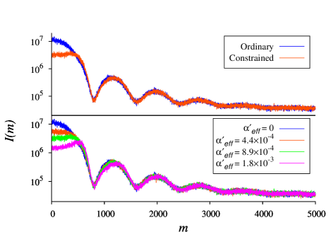
Figure 1: (Color online) Upper: Comparison of the power spectra of the ordinary and constrained TASEP with $\rho=0.1$ and $L=1000$. Lower: Constrained power spectra for $\rho=0.1$ with $L=1000$ with different $\alpha^{\prime}_{eff}$. The $\alpha^{\prime}_{eff}=0$ line corresponds to the ordinary TASEP with a constant $\alpha$.

For the other regime – crossover through SP to HD, $I_{c}$ is also severely suppressed at low $m$, though the detailed structures are less interesting. We should emphasize that, in this SP-like regime, the average $\alpha_{eff}$ is equal to $\beta$, for a range of $N_{tot}$ values. Thus, we may expect $I_{c}\sim m^{-2}$, just like in $I_{o}$ [8]. Similar to above, this expectation is indeed valid, but only for large $m$. In the suppressed region at low $m$, $I_{c}$ approaches a constant value.

4 Theoretical considerations

Since $I\left(m\right)$ carries information on time correlations of $N\left(t\right)$, even $I_{o}$ cannot be accessed from the exact stationary distribution [2]. Indeed, finding $I_{o}$ would be still a serious challenge [7], even if all the eigenvalues and the (left and right) eigenvectors of the Liouvillian (of the master equation governing TASEP) were explicitly known [6]! Thus, we will attempt to understand the suppression through a semi-phenomenological approach, similar to the one in [8]. Also based on a Langevin equation for the local particle density $\rho(x,t)$, our approach here is improved over [8] in several ways. One is the use of discrete space and time points [9], thus avoiding any issues associated with UV cutoffs. Another concerns the use of a ring of $L+1$ sites rather than open boundaries, so that any issues associated with boundary currents and noise are avoided. Finally, due to the constraint, $N\left(t\right)=N_{tot}-N_{p}\left(t\right)$, so that $I\left(m\right)$ is directly related to the fluctuations of $\rho(0,t)$, which is the pool.

For simplicity, we define $\Delta_{t}\rho(x,t)\equiv\rho(x,t+1)-\rho(x,t)$ and suppress $t$ when no ambiguity exists. For all but the “exceptional sites,” i.e., $x=0,1,$ and $L$, we may write

$$\Delta_{t}\rho(x) = \rho(x-1)[1-\rho(x)]-\rho(x)[1-\rho(x+1)]$$ (2)

$$+\xi(x-1,t)-\xi(x,t)$$

where $\xi(x,t)$ is the noise associated with the jump $x\rightarrow$ $x+1$. Next, we define $\tilde{\xi}\equiv\xi(L)-\xi(0)$ and write

$$\Delta_{t}\rho(0)=\beta\rho(L)-\alpha_{eff}\left(\rho(0)\right)[1-\rho(1)]+\tilde{\xi}\,$$ (3)

and similar equations for $\rho(1)$ and $\rho(L)$. The conservation constraint, $\sum_{x}\Delta_{t}\rho(x)=0$, can be verified. In principle, it is possible for $\rho(x\neq 0)$ to exceed unity (due to the Gaussian noise and discrete time), but we will disregard this complication here.

To simplify the computation, we choose $\alpha$, $\beta$, and $N_{tot}$ such that the system is in a LD state with a flat (average) profile, $\bar{\rho}$. For fluctuations in the lattice ($x\in\left[1,L\right]$), we write $\varphi(x,t)=\rho(x,t)-\bar{\rho}$ and, for the pool, $\zeta(t)=N_{p}(t)-\bar{N}_{p}$ (due to the conserved dynamics, $\zeta+\sum_{x}\varphi\equiv 0$). Next, we expand the equations above, keeping only linear terms in $\varphi$ and $\zeta$. Of course, we must also linearize $\alpha_{eff}$ around its average (which is, in LD, just $\bar{\rho}$):

$$\alpha_{eff}=\bar{\rho}-\alpha_{eff}^{\prime}\zeta(t)+\dots$$ (4)

The result is a standard biased diffusion equation for $\varphi$ within the lattice, along with novel equations for the exceptional sites. In this approach, the diffusion coefficient is just $1/2$ and the bias is $v\equiv 1-2\bar{\rho}$. Note that the only difference between $I_{o}$ and $I_{c}$ lies in $\alpha_{eff}^{\prime}$ in eq. (4) being zero or not. This set of linearized equations can be solved in Fourier space, with $\tilde{\varphi}(k,\omega)$, $\tilde{\zeta}(\omega)$, and $\tilde{\xi}(k,\omega)$. Deferring details to elsewhere, we present only the results along with a few remarks here.

Assuming Gaussian noise with zero mean and correlation $\langle\tilde{\xi}(k,\omega)\tilde{\xi}(k^{{}^{\prime}},\omega^{{}^{\prime}})\rangle=A\delta_{k,k^{{}^{\prime}}}\delta_{\omega,\omega^{{}^{\prime}}}$, we solve the linearized equations and obtain, in particular,

$$\langle|\tilde{\zeta}(\omega)|^{2}\rangle=\sum_{k}\frac{2A(1-\cos k)}{|Q(\omega)P(k,\omega)|^{2}}$$ (5)

where $P(k,\omega)=e^{i\omega}-\cos k+iv\sin k$ and

$$Q(\omega)=\sum_{q}\frac{e^{i\omega}-1+\alpha_{eff}^{\prime}\left(1-\bar{\rho}\right)(1-e^{-iq})}{(L+1)P(q,\omega)}$$ (6)

At this level of approximation, $A$ is usually taken as $\bar{\rho}\left(1-\bar{\rho}\right)$[13]. Recalling that the complete power spectrum is precisely $\langle|\tilde{\zeta}(\omega)|^{2}\rangle$, we can compare (5) with the simulation data. However, first we must account for a minor complication: the measurements taken only every $\ell$ MCS. Summing over the unobserved $t$’s is equivalent to summing over the harmonics $\omega_{m,\mu}=2\pi\left(\frac{m}{T}+\frac{\mu}{\ell}\right);$ $\mu=0,...,\ell-1$. A straightforward computation leads to

$$I(m)=\frac{1}{\ell^{2}}\sum_{\mu=0}^{\ell-1}\sum_{k}\frac{2A(1-\cos k)}{|Q(\omega_{m,\mu})P(k,\omega_{m,\mu})|^{2}}.$$ (7)

Note that the only difference between $I_{o}$ and $I_{c}$ is the extra term proportional to $\alpha_{eff}^{\prime}$ in $Q(\omega)$.

In previous studies [8], a similar approach led to good fits, provided an effective “renormalized” diffusion coefficient $D$ is introduced and allowed as a fit parameter. Our result, as shown in eq. (7), appears more complicated than the previous approach. But, when it is evaluated numerically, it is very similar to the earlier prediction [8] for $I_{o}\left(m\right)$. However, our UV cutoff is built in, so that there is no obvious way to insert a “renormalized” $D$ into either eq. (2) or $P(k,\omega)$. To go beyond this impasse, we plan to pursue perturbation theory seriously. Despite these unresolved issues, let us present a remarkable prediction from eq. (7) here. Instead of the individual $I$’s, consider the ratio $I_{0}/I_{c}$. For reasons yet to be understood, there is quite good agreement between the data and theoretical results. In fig. 2, we illustrate this “zero parameter fit” for these ratios in a case with $L=1000$. We should caution that the agreement in a larger system ($L=32000$), though adequate, is not as impressive. Thus, the best we may conclude at this stage is that the ratio $I_{0}/I_{c}$ is somehow less sensitive to renormalization effects.

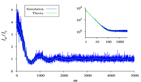
Figure 2: (Color online) Simulation data and theory for the ratio of $I_{o}$ and $I_{c}$ plotted as a function of $m$ for LD (inset for crossover in HD).

Lastly, we turn to the crossover regime in the HD case, where a DW wanders relatively freely within the lattice. The appropriate comparison case in the ordinary TASEP is SP where $I_{o}\sim m^{-2}$ [8]. Our goal here is to explain the suppression of $I_{c}$ at small $m$. A physically intuitive picture is that the DW is localized by the feedback (through $\alpha_{eff}$) in the constrained TASEP [12]. Thus, its dynamics must be well described by a noisy harmonic oscillator and $I_{c}$ should be just a Lorentzian. For a quantitative picture, we start with eq. (3) for $N_{p}\left(t\right)=\rho(0,t)$, but with the simplifying approximations $\rho(L)\cong 1-\beta$ and $\rho(1)\cong\alpha_{eff}$. For the SP in an ordinary TASEP, $\alpha_{eff}\equiv\alpha=\beta$, so that $\Delta_{t}N_{p}=\xi$ (with appropriate boundary conditions), leading to $I_{o}\propto m^{-2}$. With finite resources, a range of $N_{tot}$ produces $\alpha_{eff}\left(\bar{N}_{p}\right)=\beta$, and so, we expand the second term to $O\left(\zeta\right)$. In the continuous $t$ limit, eq. (2) becomes $\partial_{t}\zeta=-\gamma\zeta+\xi$ with $\gamma=(1-2\beta)\alpha_{eff}^{\prime}\left(\bar{N}_{p}\right)$. The solution is trivial, leading to $\langle|\tilde{\zeta}(\omega)|^{2}\rangle\propto\left(\omega^{2}+\gamma^{2}\right)^{-1}$. As above, we compare the ratios $I_{o}/I_{c}$ , for which the theory predicts

$$\frac{I_{o}(m)}{I_{c}(m)}\propto 1+\left(\frac{\gamma T}{2\pi m}\right)^{2}\text{.}$$ (8)

In fig. 2, we plot this ratio from simulation data (for $(L,\alpha,\beta,N^{*},N_{tot})$=$(1000,0.75,0.25,750,800)$) as well as the expression above. The agreement is remarkably good, especially since no fit parameters (apart from the overall proportionality constant) have been introduced. We have made such comparisons for other values of $\alpha,\beta,$ etc. and all are similar, giving us confidence that this theory is quite adequate for predicting how the feedback mechanism suppresses $I_{c}(m)$ at small $m$.

5 Summary and outlook

We studied the power spectrum associated with the total occupation, $N\left(t\right)$, on a TASEP constrained by finite resources, using both simulations and analytic techniques. Considerable suppression at low frequencies is found, depending on the feedback through $\alpha_{eff}$. Though much improved over a previous approach, the theory we studied also predicts only certain aspects of the observed spectra. Nevertheless, it is surprising that there is good agreement for the ratio of the power spectra ($I_{o}/I_{c}$), with no fit parameters!

Obviously, this approach to understanding the simulation results leaves room for improvement. We believe that the non-linear terms neglected here will be the key to better predictions, especially at higher densities where the excluded volume constraint should be more relevant. Hopefully, a full investigation of their effects will also reveal the secrets of the sensitive $L$-dependent of $D$ and $A$ found earlier [8, 14]. Beyond the study of a single TASEP coupled to a finite pool of particles, we look toward generalizations of the model which may have further implications for protein synthesis in a real cell. In particular, we should study TASEPs with large particles and inhomogeneous hopping rates [3]. We are aware of preliminary studies of the power spectra of these generalized TASEPs [15] and plan systematic investigations. Further, we should consider multiple TASEPs competing for the same pool of particles, just as many mRNA’s in a cell compete for the same pool of ribosomes. A natural question – are there winners or losers? – can be crudely answered by studying their occupations, $N_{i}\left(t\right)$, and currents, $J_{i}\left(t\right)$. Obviously, power spectra of various combinations can reveal fluctuations and cross correlations between the different quantities. Perhaps they can be exploited as a sensitive diagnostic tool for distinguishing different mechanisms that control translation. Beyond translation, we believe the study of power spectra will facilitate our understanding of non-equilibrium systems in other context, such as social networks, traffic flow, and finance.

- [1] Spitzer F., Adv. Math., 5 (1970) 246. For a recent review, see G.M. Schütz, in Phase Transition and Critical Phenomena, edited by Domb C. Lebowitz J. L., Vol. 19 (Academic, London) 2001.
- [2] Derrida B., Domany E., Mukamel D., J. Stat. Phys., 69 (1992) 667; Derrida B., Evans M. R., Hakim V., Pasquier V., J. Phys. A: Math. Gen., 26 (1993) 1493; Schütz G. M. Domany E., J. Stat. Phys., 72 (1993) 277; Schütz G. M., Phys. Rev. E, 47 (1993) 4265 and the review in [1]; Golinelli O. Mallick K., J. Phys. A: Math. Theor., 39 (2006) 12679; Blythe R. A. Evans M. R., J. Phys. A: Math. Theor., 40 (2007) R333; and also Derrida in [13]
- [3] MacDonald C., Gibbs J., Pipken A., Biopolymers, 6 (1968) 1; MacDonald C. Gibbs J. , Biopolymers, 7 (1969) 707; Shaw L. B., Zia R. K. P., Lee K. H., Phys. Rev. E, 68 (2003) 021910; Chou T. Lakatos G., Phys. Rev. Lett., 93 (2004) 198101; Dong J. J., Schmittmann B., Zia R. K. P., Phys. Rev. E, 76 (2007) 051113.
- [4] Kardar M., Parisi G., Zhang Y.-C., Phys. Rev. Lett., 56 (1986) 889; Wolf D. E. Tang L.-H., Phys. Rev. Lett., 65 (1990) 1591.
- [5] Chowdhury D., Santen L., Schadschneider A., Curr. Sci., 77 (1999) 411; Popkov V., Santen L., Schadschneider A., Schütz G. M., J. Phys. A: Math. Gen., 34 (2001) L45.
- [6] de Gier J. Essler F. H. L., J. Stat. Mech., (2006) P12011. For reviews, see those in [2].
- [7] Blythe R., private communication. Non-trivial matrix elements are needed to compute .
- [8] Adams D. A., Zia R. K. P., Schmittmann B., Phys. Rev. Lett., 99 (2007) 020601.
- [9] Pierobon P., Parmeggiani A., von Oppen F., and Frey E., Phys. Rev. E, 72 (2005) 036123.
- [10] Chou T., Biophys. J., 85 (2003) 755.
- [11] Adams D. A., Schmittmann B., Zia R. K. P, J. Stat. Mech., (2008) P06009. For a similar TASEP with fixed total particle number, see Ha M. den Nijs M., Phys. Rev. E, 66 (2002) 036118.
- [12] Cook L. J. Zia R. K. P., J. Stat. Mech., (2009) P02012.
- [13] Krug J., Phys. Rev. Lett., 67 (1991) 1882; Derrida B., J. Stat. Mech., (2007) P07023. A more sophisticated version of , , was advanced in [9].
- [14] Angel A. G. Zia R. K. P., J. Stat. Mech., (2009) P03009.
- [15] Dong J. J., private communication (2009).