Hearing the Clusters of a Graph: A Distributed Algorithm

Abstract

We propose a novel distributed algorithm to cluster graphs. The algorithm recovers the solution obtained from spectral clustering without the need for expensive eigenvalue/vector computations. We prove that, by propagating waves through the graph, a local fast Fourier transform yields the local component of every eigenvector of the Laplacian matrix, thus providing clustering information. For large graphs, the proposed algorithm is orders of magnitude faster than random walk based approaches. We prove the equivalence of the proposed algorithm to spectral clustering and derive convergence rates. We demonstrate the benefit of using this decentralized clustering algorithm for community detection in social graphs, accelerating distributed estimation in sensor networks and efficient computation of distributed multi-agent search strategies.

,

1 Introduction

In recent years, there has been great interest in the analysis of large interconnected systems, such as sensors networks, social networks, the Internet, biochemical networks, power networks, etc. These systems are characterized by complex behavior that arises due to interacting subsystems. For such systems graph theoretic methods have recently been applied and extended to study these systems. In particular, spectral properties of the Laplacian matrix associated with such graphs provide useful information for the analysis and design of interconnected systems. The computation of eigenvectors of the graph Laplacian is the cornerstone of spectral graph theory [1, 2], and it is well known that the sign of the second (and successive eigenvectors) can be used to cluster graphs [3, 4].

The problem of graph (or data, in general) clustering arises naturally in applications ranging from social anthropology [5], gene networks [6], protein sequences [7], sensor networks [8, 9, 10], computer graphics [11] and Internet routing algorithms [12].

The basic idea behind graph decomposition is to cluster nodes into groups with strong intra-connections but weak inter-connections. If one poses the clustering problem as a minimization of the inter-connection strength (sum of edge weights between clusters), it can be solved exactly and quickly [13]. However, the decomposition obtained is often unbalanced (some clusters are large and others small) [2]. To avoid unbalanced cuts, size restrictions are typically placed on the clusters, i.e., instead of minimizing inter-connection strength, we minimize the ratio of the inter-connection strength to the size of individual clusters. This, however, makes the problem NP-complete [14]. Several heuristics to partition graphs have been developed over the last few decades [15] including the Kernighan-Lin algorithm [16], Potts method [17], percolation based methods [18], horizontal-vertical decomposition [19] and spectral clustering [3, 4].

1.1 Spectral clustering

Spectral clustering has emerged as a powerful tool of choice for graph decomposition purposes (see [2] and references therein). The method assigns nodes to clusters based on the signs of the elements of the eigenvectors of the Laplacian corresponding to increasing eigenvalues [1, 3, 4]. In [20], the authors have developed a distributed algorithm for spectral clustering of graphs. The algorithm involves performing random walks, and at every step neglecting probabilities below a threshold value. The nodes are then ordered by the ratio of probabilities to node degree and grouped into clusters. Since this algorithm is based on random walks, it suffers, in general, from slow convergence rates.

Since the clustering assignment is computed using the eigenvectors/eigenvalues of the Laplacian matrix, one can use standard matrix algorithms for such computation [21]. However, as the size of the matrix (and thus the corresponding network) increases, the execution of these standard algorithms becomes infeasible on monolithic computing devices. To address this issue, algorithms for distributed eigenvector computations have been proposed [12]. These algorithms, however, are also (like the algorithm in [20]) based on the slow process of performing random walks on graphs.

1.2 Wave equation method

In a theme similar to Mark Kac’s question “Can one hear the shape of a drum?” [22], we demonstrate that by evolving the wave equation in the graph, nodes can “hear” the eigenvectors of the graph Laplacian using only local information. Moreover, we demonstrate, both theoretically and on examples, that the wave equation based algorithm is orders of magnitude faster than random walk based approaches for graphs with large mixing times. The overall idea of the wave equation based approach is to simulate, in a distributed fashion, the propagation of a wave through the graph and capture the frequencies at which the graph “resonates”. In this paper, we show that by using these frequencies one can compute the eigenvectors of the Laplacian, thus clustering the graph. We also derive conditions that the wave must satisfy in order to cluster graphs using the proposed method.

The paper is organized as follows: in Section 2 we describe current methodologies for distributed eigenvector/clustering computation based on the heat equation. In Section 3 the new proposed wave equation method is presented. In Section 4 we determine bounds on the convergence time of the wave equation. In Section 5 we show some numerical clustering results for a few graphs, including a large social network comprising of thousands of nodes and edges. We then show, in Section 6, how the wave equation can be used to accelerate distributed estimation in a large-scale environment such as a building. In Section 7 we show how the proposed distributed clustering algorithm enables one to efficiently transform a centralized search algorithm into a decentralized one. Finally, conclusions are drawn in Section 8.

2 From heat to wave equation: Related work

Let $\mathcal{G}=(V,E)$ be a graph with vertex set $V=\{1,\dots,N\}$ and edge set $E\subseteq V\times V$, where a weight ${\mathbf{W}}_{ij}\geq 0$ is associated with each edge $(i,j)\in E$, and ${\mathbf{W}}$ is the $N\times N$ weighted adjacency matrix of $\mathcal{G}$. We assume that ${\mathbf{W}}_{ij}=0$ if and only if $(i,j)\notin E$. The (normalized) graph Laplacian is defined as,

$${\mathbf{L}}_{ij}=\begin{cases}1&\mbox{if}\>i=j\\ -{\mathbf{W}}_{ij}/\sum_{\ell=1}^{N}{\mathbf{W}}_{i\ell}&\mbox{if}\>(i,j)\in E\\ 0&\mbox{otherwise}\,,\end{cases}$$ (1)

or equivalently, ${\mathbf{L}}={\mathbf{I}}-{\mathbf{D}}^{-1}{\mathbf{W}}$ where ${\mathbf{D}}$ is the diagonal matrix with the row sums of ${\mathbf{W}}$.

Note that in this work we only consider undirected graphs. The smallest eigenvalue of the Laplacian matrix is $\lambda_{1}=0$, with an associated eigenvector ${\mathbf{v}}^{(1)}=\mathbf{1}=\left[1,1,\dots,1\right]^{T}$. Eigenvalues of ${\mathbf{L}}$ can be ordered as, $0=\lambda_{1}\leq\lambda_{2}\leq\lambda_{3}\leq\cdots\leq\lambda_{N}$ with associated eigenvectors $\mathbf{1},{\mathbf{v}}^{(2)},{\mathbf{v}}^{(3)}\cdots{\mathbf{v}}^{(N)}$ [2]. It is well known that the multiplicity of $\lambda_{1}$ is the number of connected components in the graph [23]. We assume in the following that $\lambda_{1}<\lambda_{2}$ (the graph does not have disconnected clusters). We also assume that there exist unique cuts that divide the graph into $k$ clusters. In other words, we assume that there exist $k$ distinct eigenvalues close to zero [24].

Given the Laplacian matrix ${\mathbf{L}}$, associated with a graph $\mathcal{G}=(V,E)$, spectral clustering divides $\mathcal{G}$ into two clusters by computing the sign of the $N$ elements of the second eigenvector ${\mathbf{v}}^{(2)}$, or Fiedler vector [2, 4]. This process is depicted in Fig. 1 for a line graph where one edge (the edge (5,6)) has lower weight than other edges.

More than two clusters can be computed from signs of the elements of higher eigenvectors, i.e. ${\mathbf{v}}^{(3)}$, ${\mathbf{v}}^{(4)}$, etc. [2]. Alternatively, once the graph is divided into two clusters, the spectral clustering algorithm can be run independently on both clusters to compute further clusters. This process is repeated until either a desired number of clusters is found or no further clusters can be computed. This method can also be used to compute a hierarchy of clusters.

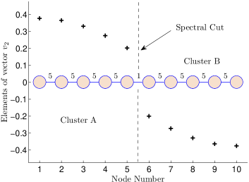
Figure 1: Spectral clustering: The sign of the $i$-th element of eigenvector $v_{2}$ determines the cluster assignment of the $i$-th vertex, demonstrated on a simple line graph example(shown in the center). With $+$ we plot the value of the components of $v_{2}$.

There are many algorithms to compute eigenvectors, such as the Lanczos method or orthogonal iteration [21]. Although some of these methods are distributable, convergence is slow [21] and the algorithms do not consider/take advantage of the fact that the matrix for which the eigenvalues and eigenvectors need to be computed is the adjacency matrix of the underlying graph. In [12], the authors propose an algorithm to compute the first $k$ largest eigenvectors (associated with the first $k$ eigenvalues with greatest absolute value) of a symmetric matrix. The algorithm in [12] emulates the behavior of orthogonal iteration. To compute the first $k$ eigenvectors of a given matrix ${\mathbf{J}}$, at each node in the network, matrix ${\mathbf{V}}_{i}=\sum_{j\in\mathcal{N}(i)}{\mathbf{J}}_{ij}{\mathbf{Q}}_{j}$ is computed, where ${\mathbf{Q}}_{j}\in\mathds{R}^{N\times k}$ is initialized to a random matrix and $\mathcal{N}(i)$ is the set of neighbors of node $i$ (including node $i$ itself). Orthonormalization is achieved by the computation of matrix ${\mathbf{K}}_{i}={\mathbf{V}}_{i}^{T}{\mathbf{V}}_{i}$ at every node, followed by computation of matrix ${\mathbf{K}}$, which is the sum of all the ${\mathbf{K}}_{i}$ matrices in the network. Once matrix ${\mathbf{K}}$ is computed, ${\mathbf{Q}}_{i}={\mathbf{V}}_{i}{\mathbf{R}}^{-1}$ is updated at each node, where ${\mathbf{R}}$ is a unique matrix such that ${\mathbf{K}}={\mathbf{R}}^{T}{\mathbf{R}}$ (Cholesky decomposition). The above iteration is repeated until ${\mathbf{Q}}_{i}$ converges to the $i$-th eigenvector. The sum of all the matrices ${\mathbf{K}}_{i}$ is done in a decentralized way, using gossip [25], which is a deterministic simulation of a random walk on the network. In particular, at each node one computes the matrix ${\mathbf{K}}$ as follows,

$${\mathbf{S}}_{i}(t+1) =\sum_{j\in\mathcal{N}(i)}{\mathbf{B}}_{ji}{\mathbf{S}}_{j}(t)\,,$$ (2)

$$\boldsymbol{\pi}_{i}(t+1) =\sum_{j\in\mathcal{N}(i)}{\mathbf{B}}_{ji}\boldsymbol{\pi}_{j}(t)\,,$$ (3)

for $t\geq\tau$ steps, where $\tau$ is the mixing time for the random walk on the graph [12]. Here ${\mathbf{K}}={\mathbf{S}}_{i}/\boldsymbol{\pi}_{i}$, ${\mathbf{S}}_{i}(0)={\mathbf{K}}_{i}$ and $\boldsymbol{\pi}_{i}(0)=1$ for only one index $i$ and zero for other indices. The values ${\mathbf{B}}_{ij}$ are transition probabilities of the Markov chain associated with the graph. A natural choice is ${\mathbf{B}}_{ij}=1/\mbox{deg}(i)$, where $\mbox{deg}(i)$ is the degree of node $i$. Note that matrix ${\mathbf{B}}=[{\mathbf{B}}_{ij}]$ is the normalized adjacency matrix (given by ${\mathbf{D}}^{-1}{\mathbf{W}}$). This algorithm converges after $O(\tau\log^{2}N)$ iterations [12].

The slowest step in the distributed computation of eigenvectors is the simulation of a random walk on the graph (defined by Eq. 2 and 3). It is clear from Eq. 1 that successive multiplications by the adjacency matrix ${\mathbf{B}}$ in Eqs. 2 and 3 are equivalent to successive multiplications by matrix ${\mathbf{I}}-{\mathbf{L}}$. This procedure is equivalent to evolving the discretized heat equation on the graph and can be demonstrated as follows. The heat equation is given by,

$$\frac{\partial u}{\partial t}=\Delta u\,,$$

where $u$ is a function of time and space, $\partial u/\partial t$ is the partial derivative of $u$ with respect to time, and $\Delta$ is the Laplace operator [26]. When the above equation is discretized (see [1, 27, 28, 29] for details) on a graph $\mathcal{G}=(V,E)$ one gets the following equation:

$${\bf u}_{i}(t+1)={\bf u}_{i}(t)-\displaystyle\sum_{j\in\mathcal{N}(i)}{\mathbf{L}}_{ij}{\bf u}_{j}(t)\,,$$

for $i,j\in V$. Here ${\bf u}_{i}(t)$ is the scalar value of $u$ on node $i$ at time $t$. The graph Laplacian ${\mathbf{L}}=[{\mathbf{L}}_{ij}]$ appears due to the discretization of the $\Delta$ operator [28]. The above iteration can be re-written, in matrix form, ${\bf u}(t+1)=({\mathbf{I}}-{\mathbf{L}})\,{\bf u}(t)$ where ${\bf u}(t)=({\bf u}_{1}(t),\dots,{\bf u}_{N}(t))^{T}$. The solution of this iteration is,

$${\bf u}(t)=C_{0}\mathbf{1}+C_{1}(1-\lambda_{2})^{t}{\mathbf{v}}^{(2)}+\dots+C_{N}(1-\lambda_{N})^{t}{\mathbf{v}}^{(N)}\,,$$ (4)

where constants $C_{j}$ depend on the initial condition ${\bf u}(0)$. It is interesting to note that in Eq. 4, the dependence of the solution on higher eigenvectors and eigenvalues of the Laplacian decays with increasing iteration count. Thus, it is difficult to devise a fast and distributed method for clustering graphs based on the heat equation. Next, we derive a novel algorithm based on the idea of permanent excitation of the eigenvectors of ${\mathbf{I}}-{\mathbf{L}}$. We note that the above connection between spectral clustering and the heat equation is not new and was pointed out in [30, 31].

Before discussing the details of wave-equation based eigenvector computation, we remark that in [32] the authors have independently developed a decentralized algorithm to compute the eigenvalues of the Laplacian. Compared to our approach, their algorithm involves solving a fourth order partial differential equation on the graph. This imposes twice the cost of communication, computation and memory on every node in the graph.

3 Wave equation based computation

Consider the wave equation,

$$\frac{\partial^{2}u}{\partial t^{2}}=c^{2}\Delta u\,.$$ (5)

Analogous to the heat equation case (Eq. 4), the solution of the wave equation can be expanded in terms of the eigenvectors of the Laplacian. However, unlike the heat equation where the solution eventually converges to the first eigenvector of the Laplacian, in the wave equation all the eigenvectors remain eternally excited [26] (a consequence of the second derivative of $u$ with respect to time). Here we use this observation to develop a simple, yet powerful, distributed eigenvector computation algorithm. The algorithm involves evolving the wave equation on the graph and then computing the eigenvectors using local FFTs. Note that some properties of the wave equation on graphs have been studied in [33]. Here we construct a graph decomposition/partitioning algorithm based on the discretized wave equation on the graph, given by

$${\bf u}_{i}(t)=2{\bf u}_{i}(t-1)-{\bf u}_{i}(t-2)-c^{2}\displaystyle\sum_{j\in\mathcal{N}(i)}{\mathbf{L}}_{ij}{\bf u}_{j}(t-1)\,,$$ (6)

where $\sum_{j\in\mathcal{N}(i)}{\mathbf{L}}_{ij}{\bf u}_{j}(t-1)$ originates from the discretization of $\Delta u$ in Eq. 5, see [28] for details. The rest of the terms originate from discretization of $\partial^{2}u/\partial t^{2}$. To update ${\bf u}_{i}$ using Eq. 6, one needs only the value of ${\bf u}_{j}$ at neighboring nodes and the connecting edge weights (along with previous values of ${\bf u}_{i}$).

The main steps of the algorithm are shown as Algorithm 3.1. Note that at each node (node $i$ in the algorithm) one only needs nearest neighbor weights ${\mathbf{L}}_{ij}$ and the scalar quantities ${\bf u}_{j}(t-1)$ also at nearest neighbors. We emphasize, again, that ${\bf u}_{i}(t)$ is a scalar quantity and Random($[0,1]$) is a random initial condition on the interval $[0,1]$. The vector ${\mathbf{v}}^{(j)}_{i}$ is the $i$-th component of the $j$-th eigenvector, $T_{max}$ is a positive integer derived in Section 4, FrequencyPeak(Y,j) returns the frequency at which the $j$-th peak occurs and $\texttt{Coefficient}(\omega_{j})$ return the corresponding Fourier coefficient.

Algorithm 3.1 Wave equation based eigenvector computation algorithm for node $i$. At node $i$ one computes the sign of the $i$-th component of the first $k$ eigenvectors. The cluster assignment is obtained by interpreting the vector of $k$ signs as a binary number.

1:${\bf u}_{i}(0)\leftarrow\texttt{Random}\>([0,1])$

2:${\bf u}_{i}(-1)\leftarrow{\bf u}_{i}(0)$

3:$t\leftarrow 1$

4:while $t<T_{max}$ do

5:     

${\bf u}_{i}(t)\leftarrow 2{\bf u}_{i}(t-1)-{\bf u}_{i}(t-2)-$

$\qquad\qquad c^{2}\sum_{j\in\mathcal{N}(i)}{\mathbf{L}}_{ij}{\bf u}_{j}(t-1)$

6:     $t\leftarrow t+1$

7:end while

8:$Y\leftarrow\texttt{FFT}\>(\left[{\bf u}_{i}(1),\dots\dots,{\bf u}_{i}(T_{max})\right])$

9:for $j\in\{1,\dots,k\}$ do

10:     $\omega_{j}\leftarrow\texttt{FrequencyPeak}\>(Y,j)$

11:     ${\mathbf{v}}^{(j)}_{i}\leftarrow\texttt{Coefficient}(\omega_{j})$

12:     if ${\mathbf{v}}^{(j)}_{i}>0$ then

13:         $A_{j}\leftarrow 1$

14:     else

15:         $A_{j}\leftarrow 0$

16:     end if

17:end for

18:ClusterNumber $\leftarrow\sum_{j=1}^{k}A_{j}2^{j-1}$

Proposition 3.1.

The wave equation iteration (6) is stable on any graph if the wave speed satisfies the following inequality,

$$0<c<\sqrt{2}\,,$$

with an initial condition of ${\bf u}(-1)={\bf u}(0)$.

For analysis of the algorithm, we consider Eq. 6 in vector form,

$${\bf u}(t)=-{\bf u}(t-2)+(2{\mathbf{I}}-c^{2}{\mathbf{L}}){\bf u}(t-1)\,.$$ (7)

We stress again that, in practice, the algorithm is distributed and at every node one updates the state based on Eq. 6. The update equations given by Eq. 6 (and Eq. 7) correspond to discretization of Eq. 5 with Neumann boundary conditions [34].

One can write iteration Eq. 7 in matrix form,

$$\underbrace{\begin{pmatrix}{\bf u}(t)\\ {\bf u}(t-1)\end{pmatrix}}_{\mathbf{z}(t)}=\underbrace{\begin{pmatrix}2{\mathbf{I}}-c^{2}{\mathbf{L}}&-{\mathbf{I}}\\ {\mathbf{I}}&0\end{pmatrix}}_{\mathbf{M}}\underbrace{\begin{pmatrix}{\bf u}(t-1)\\ {\bf u}(t-2)\end{pmatrix}}_{\mathbf{z}(t-1)}\,.$$ (8)

This implies that,

$$\mathbf{z}(t)={\mathbf{M}}^{t}\mathbf{z}(0)\,,$$ (9)

where $\mathbf{z}(0)=({\bf u}(0),{\bf u}(-1))^{T}$. We now analyze the solution to Eq. 9 in terms of the eigenvalues and eigenvectors of the graph Laplacian ${\mathbf{L}}$.

We can compute the eigenvectors of ${\mathbf{M}}$ by solving for a generic vector $({\bf a}_{j},{\bf b}_{j})^{T}$,

$${\mathbf{M}}\begin{pmatrix}{\bf a}_{j}\\ {\bf b}_{j}\end{pmatrix}=\alpha_{j}\begin{pmatrix}{\bf a}_{j}\\ {\bf b}_{j}\end{pmatrix}\,.$$

This implies that the eigenvectors of  ${\mathbf{M}}$ are given by,

$${\mathbf{m}}^{(j)}=\begin{pmatrix}\alpha_{j}\>{\mathbf{v}}^{(j)}\\ {\mathbf{v}}^{(j)}\end{pmatrix}\,,$$ (10)

with eigenvalues

$$\alpha_{j_{1,2}}=\frac{2-c^{2}\lambda_{j}}{2}\pm\frac{c}{2}\sqrt{c^{2}\lambda_{j}^{2}-4\lambda_{j}}\,.$$ (11)

It is evident from Eq. 11 that stability is obtained if and only if,

$$\left|\frac{2-c^{2}\lambda_{j}}{2}\pm\frac{\sqrt{(2-c^{2}\lambda_{j})^{2}-4}}{2}\right|\leq 1\,.$$

The absolute value from the above equation is plotted for various values of $\theta_{j}=2-c^{2}\lambda_{i}$, in Fig. 2. The above stability condition is satisfied for $-2\leq\theta_{j}\leq 2$, which yields the following bound on $c$:

$$0\leq c\leq\frac{2}{\sqrt{\lambda_{i}}}\,.$$

The above equation must hold true for all eigenvalues of ${\mathbf{L}}$. The most restrictive of which is $c\leq 2/\sqrt{\lambda_{N}}$. Since $\lambda_{N}\leq 2$ for all graphs,

$$0\leq c\leq\sqrt{2}\,,$$

guarantees that all the eigenvalues of ${\mathbf{M}}$ have absolute value equal to one.

\psfrag{a}{$\theta_{j}$}\psfrag{b}[b]{$\left|\cfrac{\theta_{j}}{2}\pm\cfrac{\sqrt{(\theta_{j})^{2}-4}}{2}\right|$}\includegraphics[width=184.28981pt]{absval2_new.eps}

Figure 2: Plot of functions $|\theta_{j}/2\pm 1/2\sqrt{(\theta_{j})^{2}-4}|$. Blue (dashed) line is the function with a negative second term. Red (solid) line is the function with a positive second term.

However, Eqn. 6 will be unstable if any of the eigenvalues of ${\mathbf{M}}$ have geometric multiplicity strictly less than the algebraic multiplicity with an initial condition that has non-zero projection on the unstable generalized eigenvectors. We now derive conditions so that these instabilities do not arise.

From Eqn. 11 it is evident that there are three cases to analyze.

Case i):

Since ${\mathbf{L}}$ always has an eigenvalue at 0, this implies that ${\mathbf{M}}$ always has an eigenvalue at 1 with algebraic multiplicity two. It can be shown that the geometric multiplicity of this eigenvalue is equal to one. The corresponding eigenvector is $\mathbf{1}_{2N\times 1}$, with a generalized eigenvector $(\mathbf{1},-\mathbf{1})^{T}$. To avoid instability, the initial conditions must be of the form $({\bf u}(0),{\bf u}(0))^{T}$. In other words, we set ${\bf u}(-1)={\bf u}(0)$ to ensure that the initial condition is orthogonal to $(\mathbf{1},-\mathbf{1})^{T}$.

Case ii):

If ${\mathbf{L}}$ has $k$ repeated eigenvalues, it implies that ${\mathbf{M}}$ has $k$ repeated eigenvalues. In this case, however, the geometric and algebraic multiplicities are equal. One can show that the matrix ${\mathbf{L}}$ is similar to the symmetric matrix,

$${\mathbf{L}}_{sym}={\mathbf{D}}^{-1/2}({\mathbf{D}}-{\mathbf{W}}){\mathbf{D}}^{-1/2}\,,$$

(in particular, ${\mathbf{L}}={\mathbf{D}}^{-1/2}{\mathbf{L}}_{sym}{\mathbf{D}}^{1/2}$), implying that ${\mathbf{L}}$ is diagonalizable. Thus, the eigenvectors of ${\mathbf{L}}$ associated with the repeated eigenvalues are linearly independent. Since matrix ${\mathbf{M}}$ has eigenvectors of the form shown in Eqn. 10, the repeated eigenvalues of ${\mathbf{M}}$ have eigenvectors that are linearly independent.

Case iii):

The matrix ${\mathbf{M}}$ has a repeated eigenvalue at -1 if  $c^{2}=2$ and $\lambda_{N}=2$. This repeated eigenvalue has an associated eigenvector $(-{\mathbf{v}}_{N},{\mathbf{v}}_{N})^{T}$ and a generalized eigenvector $({\mathbf{v}}_{N},{\mathbf{v}}_{N})^{T}$. Clearly, in this case the initial condition would need to be orthogonal to both the vector $(\mathbf{1},-\mathbf{1})^{T}$ and the vector $({\mathbf{v}}_{N},{\mathbf{v}}_{N})^{T}$. This can be achieved if and only if ${\bf u}(0)\bot{\mathbf{v}}_{N}$ and ${\bf u}(-1)={\bf u}(0)$. This is an undesirable condition, as it requires prior knowledge of ${\mathbf{v}}_{N}$. We avoid this situation by setting $c<\sqrt{2}$.

Thus, we can guarantee stability of the wave equation iteration on any graph (given by Eqn. 6), as long as $0<c<\sqrt{2}$ and the initial condition has the form ${\bf u}(-1)={\bf u}(0)$.

Notice that the condition ${\bf u}(-1)\neq{\bf u}(0)$ is analogous to a non-zero initial derivative condition on $u$ for the continuous PDE, which is known to give a solution that grows in time [26].

Remark 3.2.

Although we call $c$ the wave speed, it only controls the extent to which neighbors influence each other and not the speed of information propagation in the graph.

Proposition 3.3.

The clusters of graph $\mathcal{G}$, determined by the signs of the elements of the eigenvectors of ${\mathbf{L}}$, can be computed using the frequencies and coefficients obtained from the Fast Fourier Transform of $({\bf u}_{i}(1),\dots,{\bf u}_{i}(T_{max}))$, for all $i$ and some $T_{max}>0$. Here ${\bf u}_{i}$ is governed by the wave equation on the graph with the initial condition ${\bf u}(-1)={\bf u}(0)$ and $0<c<\sqrt{2}$.

We can write the eigenvectors ${\mathbf{m}}^{(j)}$ of ${\mathbf{M}}$ as,

$${\mathbf{m}}^{(j)}={\mathbf{p}}^{(j)}\pm i{\mathbf{q}}^{(j)}\,,$$

where,

$${\mathbf{p}}^{(j)}=\begin{pmatrix}\mathrm{Real}(\alpha_{j}){\mathbf{v}}^{(j)}\\ {\mathbf{v}}^{(j)}\end{pmatrix}\,,\quad{\mathbf{q}}^{(j)}=\begin{pmatrix}\textrm{Imag}(\alpha_{j}){\mathbf{v}}^{(j)}\\ 0\end{pmatrix}\,.$$

Using $\alpha_{j}=e^{i\omega_{j}}$, we can represent the solution of the update equation (Eqn. 6), or equivalently,

$$\mathbf{z}(t)={\mathbf{M}}^{t}\mathbf{z}(0)\,,$$ (12)

by expanding $\mathbf{z}(0)$ in terms of ${\mathbf{p}}^{(j)}$ and ${\mathbf{q}}^{(j)}$. Recall, that $\mathbf{z}(0)=({\bf u}(0),{\bf u}(0))^{T}$ is orthogonal to the generalized eigenvector $(\mathbf{1},-\mathbf{1})^{T}$. Thus, $\mathbf{z}(0)$ is represented as a linear combination of $(\mathbf{1},\mathbf{1})^{T}$ and ${\mathbf{m}}^{(j)}$ for $j\geq 2$. This implies that the solution to Eqn. 8 and 9 is given by,

$$\mathbf{z}(t)=\sum_{j=1}^{N}C_{j_{1}}\left[{\mathbf{p}}^{(j)}\cos(t\omega_{j})-{\mathbf{q}}^{(j)}\sin(t\omega_{j})\right]$$

$$+\;C_{j_{2}}\left[{\mathbf{p}}^{(j)}\sin(t\omega_{j})+{\mathbf{q}}^{(j)}\cos(t\omega_{j})\right]\,,$$ (13)

where

$$C_{j_{1}}=\mathbf{z}(0)^{T}{\mathbf{p}}^{(j)}\,,\quad C_{j_{2}}=\mathbf{z}(0)^{T}{\mathbf{q}}^{(j)}\,.$$ (14)

It is easy to see that at every node, say the $i$-th node, one can locally perform an FFT on $({\bf u}_{i}(1),\dots,{\bf u}_{i}(T_{max}))$ (where each value is computed using the update law in Eq. 6) to obtain the eigenvectors. At the $i$-th node of the graph, one computes the $i$-th component of every eigenvector from the coefficients of the FFT. More precisely, for node $i$, the coefficient of $\cos(t\omega_{j})$ is given $(C_{j_{1}}+C_{j_{2}}){\mathbf{v}}_{i}^{(j)}$. The sign of the coefficients of the eigenvector(s) provide the cluster assignment(s).

Remark 3.4.

The above algorithm assumes that one excites every frequency (or depending on the number of clusters, at least the first $k$ frequencies). This is achieved if $\mathbf{z}(0)$ is not orthogonal to ${\mathbf{p}}^{(j)}$ and ${\mathbf{q}}^{(j)}$ ($C_{j_{1}}$ and $C_{j_{2}}$ must be non-zero). As mentioned before, an initial condition of the form $\mathbf{z}(0)=({\bf u}(0),{\bf u}(0))^{T}$ prevents linear growth of the solution, however, ${\bf u}(0)$ should also not be orthogonal to ${\mathbf{v}}^{(2)},{\mathbf{v}}^{(3)}\dots\mathbf{v}^{(k)}$. This is easy to guarantee (with probability one) by picking a random initial condition at each node.

Remark 3.5.

Note that the wave equation can also be used as a distributed algorithm for eigenvector and eigenvalue computation of ${\mathbf{L}}$. From the FFT we can compute $\omega_{j}$ which in turn allows us to compute the eigenvalues $\lambda_{j}$. The eigenvector components are computed using the coefficients of $\cos(t\omega_{j})$ (or equivalently $\sin(t\omega_{j})$).

Remark 3.6.

The algorithm is also attractive from a communication point of view. In [12] entire matrices need to be passed from one node to another. In our algorithm only scalar quantities ${\bf u}_{j}$ need to be communicated.

Remark 3.7.

Peak detection algorithms based on the FFT are typically not very robust because of spectral leakage. As we are only interested in the frequencies corresponding to peaks, algorithms like multiple signal classification [35] can overcome these difficulties. The investigation of such algorithms, as well as windowing methods, is the subject of future work.

4 Performance analysis

An important quantity related to the wave equation based algorithm is the time needed to compute the eigenvalues and eigenvectors components. The distributed eigenvector algorithm proposed in [12] converges at a rate of $O(\tau\log^{2}(N))$ , where $\tau$ is the mixing time of the Markov chain associated with the random walk on the graph. We derive a similar convergence bound for the wave equation based algorithm.

It is evident from Eq. 13 that one needs to resolve the lowest frequency to cluster the graph. Let us assume that one needs to wait for $\eta$ cycles of the lowest frequency to resolve it successfully (i.e. the number of cycles needed for a peak to appear in the FFT). The time needed to cluster the graph based on the wave equation is,

$$T_{max}=\frac{\eta}{\omega_{2}}\,.$$ (15)

From Eq. 11 it is easy to see that $\cos(\omega_{2})=\mathrm{Real}(\alpha_{2})=(2-c^{2}\lambda_{2})/2$. Note that in [36] it was shown that $\tau=-(\log{|1-\lambda_{2}|})^{-1}$. Thus, it follows that,

$$\omega_{2}=\arccos\left(\frac{2+c^{2}(e^{-1/\tau}-1)}{2}\right)\,.$$

Hence, the convergence of the wave equation based eigenvector computation depends on the mixing time of the underlying Markov chain on the graph, and is given by,

$$T_{max}=O\left(\arccos\left(\cfrac{2+c^{2}(e^{-1/\tau}-1)}{2}\right)^{-1}\right)\,.$$ (16)

In the wave equation based clustering computation, one can at the $i$-th node, compute the $i$-th component of every eigenvector (along with all the eigenvalues) of the graph Laplacian, thus assigning every node to a cluster. If one uses the wave equation to compute eigenvectors, to ensure that at every node one has entire eigenvectors, an extra communication step needs to be added. As a final step, locally computed eigenvectors components are transmitted to all other nodes. The cost of this step is $O(N)$ (worst case). Thus, convergence of the distributed eigenvectors computation scales as,

$$T_{max}=O\left(\arccos\left(\cfrac{2+c^{2}(e^{-1/\tau}-1)}{2}\right)^{-1}\right)+O(N)\,.$$ (17)

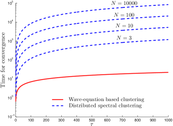
Figure 3: Comparison of convergence rates between the distributed algorithm in [12] and our proposed wave equation algorithm for $c^{2}=1.99$. The wave equation based algorithm has better scaling with $\tau$ for graphs of any size (given by $N$). The plots are upper bounds on the convergence speed.

Note that simple analysis shows that for large $\tau$ our algorithm has a convergence rate of $\sqrt{\tau}/c$ (as $O(N)$ gets dominated by $\tau$). It is interesting to note that in the discretized wave equation, though the constant $c$ loses the meaning of wave speed (that it has in the continuous case) it does impact the speed of convergence.

The convergence of wave equation based clustering is compared to convergence of distributed spectral clustering in Fig. 3, for $c^{2}=1.99$. In particular, the figure shows that wave equation based clustering has, in general, better scaling, with respect to $\tau$, than [12].

Note that the proximity of $\omega_{3}$ to $\omega_{2}$ (or the proximity of $\lambda_{3}$ to $\lambda_{2}$) will influence the constant in Eq. 16. The resolution of the FFT is $O(1/K)$, where $K$ is the number of samples. Thus, $K$ has to exceed $1/|\omega_{3}-\omega_{2}|$, to enable computation of two separate peaks. The closer $\lambda_{3}$ is to $\lambda_{2}$, the greater are the number of samples that each node needs to store in order to obtain a good estimate of $\omega_{2}$ using the FFT. A similar constant depending on the ratio of $\lambda_{2}$ and $\lambda_{3}$ arises in distributed spectral clustering [12] and any power iteration based scheme for eigenvector computation [21].

Practically, if the lowest frequency of the FFT does not change for a pre-defined length of time, we assume that convergence has been achieved.

From Eq. 16 it seems that the proposed clustering algorithm is independent of the size of the graph (since $\sqrt{\tau}/c$ dominates $O(N)$). This, however, is not true. Larger graphs with low connectivity tend to have higher mixing times. Take for example, a cyclic graph $\mathcal{C}_{N}$ shown in Fig. 4. We use the cyclic graph as a benchmark as one can explicitly compute the mixing time as a function of $N$ and make a comparison with [12]. Of course, no unique spectral cut exists for such a graph. The second eigenvalue of the Laplacian for $\mathcal{C}_{N}$ is given by,

$$\lambda_{2}=1-\cos\left(\frac{2\pi}{N}\right).$$ (18)

Thus, the mixing time of the Markov chain is given by,

$$\tau=-\frac{1}{\ln\left(\cos\left(2\pi/N\right)\right)}\approx\left(\frac{N}{2\pi}\right)^{2}\,.$$ (19)

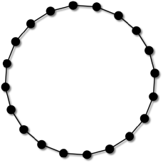
Figure 4: The ring graph $\mathcal{C}_{N}$ with $N$ nodes. Every edge has a weight of $1$.

From Eq. 16, one can show that the time for convergence of the wave equation is,

$$T_{max}=\frac{\eta}{\arccos(1+0.5c^{2}(\cos(2\pi/N)-1))}\approx\eta\frac{N}{2\pi}\,.$$ (20)

As expected, Eq. 20 predicts that as the graph becomes larger, the convergence time for the wave equation based algorithm increases. We numerically compute and compare the convergence times for random walks and wave equation on the cyclic graph (by explicitly running the iterations for both processes and checking for convergence). The results are shown in Fig. 5.

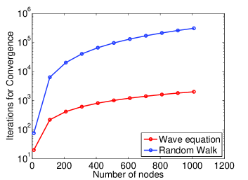
Figure 5: Convergence of random walk and wave equation on the cyclic graph $\mathcal{C}_{N}$ as a function of number of nodes, $N$.

5 Numerical results

Since our algorithm should predict the same partitions as spectral clustering, we demonstrate the algorithm on illustrative examples. Our first example, is the simple line graph shown in Fig. 6. Nodes $1$ to $100$ and $101$ to $200$ are connected to their nearest neighbors with edge weight $1$. The edge between nodes $100$ and $101$ has weight $0.1$. As expected, spectral clustering predicts a cut between nodes $100$ and $101$. We propagate the wave on the graph using update Eq. 6 at every node. At each node, one then performs an FFT on the local history of ${\bf u}$. The FFT frequencies are the same for all nodes (evident from Eq. 13) and shown in Fig. 7. The sign of the coefficients of the lowest frequency in the FFT are shown in Fig. 8. It is evident from this figure that the sign of the coefficients change sign exactly at the location of the weak connection, predicting a cut between nodes $100$ and $101$ (consistent with spectral clustering).

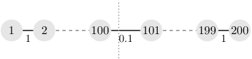
Figure 6: A line graph with nearest neighbor coupling. The edge between $100$ and $101$ is a weak connection with weight $0.1$, all other edges have weight $1.0$. Vertical line shows the predicted cut.

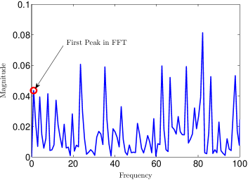
Figure 7: FFT of $\left[{\bf u}_{i}(1)\dots\bf u_{i}(T)\right]$ for any node $i$ of the line graph. Red circle marks the lowest frequency.

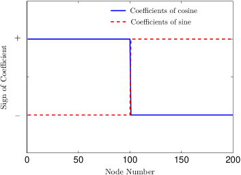
Figure 8: Signs of the coefficients of the lowest frequency for the line graph.

We now demonstrate our distributed wave equation based clustering algorithm on the Zachary Karate club graph [37] and on a Fortunato benchmark example [38]. These social networks are defined by the adjacency matrix that is determined by social interactions. We assume that all the edges have weight $1$.

W. Zachary, a sociologist, was studying friendships at a Karate club when it split into two. As expected, members picked the club with more friends. This example serves as an ideal test bed for clustering algorithms. Any effective clustering algorithm is expected to predict the observed schism. Community detection and graph clustering algorithms are routinely tested on this example, see [15, 39, 40, 41] for a few such demonstrations.

We first apply spectral clustering on this example, then run our wave equation based clustering algorithm, and compare the results in Fig. 9. As expected, we find that both algorithms partition the graph into exactly the same clusters.

We also demonstrate our algorithm on a large Fortunato benchmark with $1000$ nodes and $99084$ edges. The graph has two natural clusters with $680$ and $320$ nodes respectively. These clusters are shown in Fig. 10. The wave equation based clustering computes the graph cut exactly.

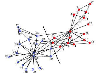
Figure 9: Graph decompositions predicted by spectral and wave equation based clustering algorithms. Both methods predict the same graph cut.

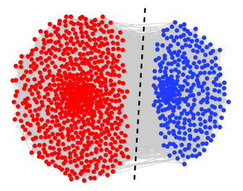
Figure 10: A Fortunato community detection benchmark with $1000$ nodes and $99084$ edges. Wave equation based clustering computes the graph cut exactly.

Thus, wave equation based eigenvector computation can be used to partition both abstract graphs on parallel computers, or physical networks such as swarms of unmanned vehicles, sensor networks, embedded networks or the Internet. This clustering can aid communication, routing, estimation and task allocation.

We now show how clustering can be effectively used to accelerate distributed estimation and search algorithms.

6 Distributed estimation over clusters

Distributed estimation has recently received significant attention see [42]–[45] and references therein. Distributed estimation algorithms require the entire network of sensors to exchange (through nearest neighbor communication) data about the measured variables in order to obtain an overall estimate, which is asymptotically (in the number of iterations) optimal. This results in estimators with error dynamics that converge to zero very slowly. It is well known that these type of algorithm can be accelerated using multi-scale approaches, see for example [46, 47, 48]. The key idea in these multi-scale approaches is to partition the sensor network into clusters, solve the distributed problem in each cluster and fuse the information between clusters.

As the overall estimation process is distributed, it is desirable that the multi-scale speedup is achieved through a distributed process as well. This means that the clustering must be computed, in a bottom-up fashion, from the structure of the network. We show in the following a simple yet illustrative example, where the wave equation based clustering algorithm can be used to accelerate distributed estimation computation by exploiting properties of the overall sensor network.

We consider the contaminant transport problem in a building [46] with two floors, each divided into 64 cells/rooms (see Fig. 11). A sensor, to detect the contaminant, is present in each cell. Sensors can communicate if their relative distance is less than 10m. However, we assume that only four sensors can communicate between floors, namely those placed within common staircases connecting the two floors. On the first floor, sensors can communicate across the empty space in between (we assume that windows are present), whereas on the second floor we assume that there are walls that reduce the communication range. We further assume that walls marked with a thick black line, see Fig. 11, degrade communication between the nodes that are inside the area to those outside.

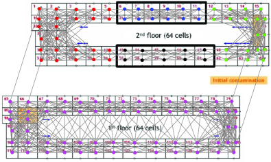
Figure 11: A two floor building subdivided into 64 cells/rooms for each floor. In each room there is a sensor node capable of communicating with neighbors within a radius of 10m. The thick black line, depicts walls that degrade communication strength.

As in [46], we assume that the contaminant is produced in four rooms, two on the first floor and two on the second. Under the simplifying assumption of perfect mixing within each cell/room volume, the contaminant propagates within the building (see [46] for details) according to:

$$\rho_{i}V_{i} \frac{dC_{i}}{dt}=\sum_{i\sim j}{F_{ji}C_{j}}-\sum_{i\sim j}{F_{ij}C_{i}}+G_{i}-R_{i}C_{i}\,,$$

$$\rho\text{ : } \text{Density}\qquad C\text{ : }\text{Contaminant concentration}$$

$$V\text{ : } \text{Volume}\qquad F_{ji}\text{ : }\text{Mass flow rate from node $j$ to $i$}$$

$$G\text{ : }$$ Contaminant generation rate

$$R\text{ : } \text{Mass removal rate}\,.$$

A constant inward flow of air is introduced at a corner of the second floor, and outflow openings exist wherever windows are open to the outside. We consider a distributed Kalman filter as one that uses consensus to average the estimates and covariance matrices between Kalman filter updates, see [46] for details.

The idea of using the wave equation for distributed clustering is to “discover” in a bottom-up fashion, the presence of clusters and exploit strong inter-cluster connectivity to accelerate computation. In particular, we demonstrate the benefit of using the “bottom-up” approach. In the building example there are two main clusters (first and second floors), which a filter and network designer can a-priori assume to know. The four clusters on the second floor, however, would not be known to the designer unless extensive communication measurements are carried out.

In order to determine the four clusters based on SNR, on the second floor, the wave equation based clustering was run for 600 steps. The clustering clearly needs to be run only once, unless there is very strong variation of SNR or the network. In this particular example we assume that the SNR and the network do not vary.

6.1 Numerical results

Numerical results are obtained by running the Kalman filter interleaved with the consensus step, see [46]. We fix 10 iterations for the consensus step in each cluster. Fig. 12 shows the estimation result for 100 updates of the Kalman filter for both clustering strategies described previously. In particular, Figs. 12a and 12b show the estimate (solid line) of the concentration (the true value is shown with dash-dot line) in room 49 made by all the sensors in the building. It can be clearly seen that the estimate in Fig. 12a is not as accurate as the one in Fig. 12b. The reason is that the consensus step for the case of four clusters on the second floor converges much faster to the true covariance compared to the case of two clusters. In comparison, if consensus is run for the case of two clusters, it requires more than 500 iterations in each consensus step to converge to the accuracy of Fig. 12b.

In the $5$ cluster case, all the nodes in the building have accurate estimates of the contaminant concentration for rooms located on the first floor. This is because sensors on the first floor are strongly connected to one another and 10 iterations are enough to converge to the true covariance (with only slight corruption by the “unconverged” averaging on the second floor).

These simulations show that the wave equation based clustering provides an efficient distributed bottom-up methodology for partitioning sensor networks and accelerating distributed estimation algorithms.

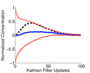
(a) Two Clusters

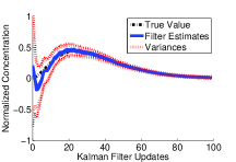
(b) Five Clusters

Figure 12: Concentration estimates for room 49. Concentration estimates (solid line) are compared to the true value (dash-dot line). The dashed lines give the $\pm 3\sigma$ curves around the estimate. As it is clear from the plots, the strategy in which the consensus step is run using five clusters (b) is much better than using two clusters (a).

7 Mobile Sensor Networks

We demonstrate the utility of distributed partitioning for computing the trajectories of mobile sensors/vehicles for the purpose of efficiently searching a large area. In [49] the authors have developed an algorithm to optimally search a region, given a prior distribution that models the likelihood of finding the target in any given location (see for example Fig. 13). The trajectories are computed using a set of ordinary differential equations given by,

$$\dot{x}_{j}(t)=u_{j}(t)\,.$$ (21)

The above equation describes the dynamics of the $j$-th vehicle, where $x_{j}(t)$ and $u_{j}(t)$ are the position and the control input of the $j$-th vehicle at time $t$ respectively. The authors prove that the control law

$$u_{j}(t)=-u_{max}\frac{B_{j}(t)}{||B_{j}(t)||}\,,$$ (22)

efficiently samples the prior distribution for search. Here,

$$B_{j}(t)=\sum_{k}\frac{\Lambda_{k}S_{k}(t)\nabla f_{k}(x_{j}(t))}{\langle f_{k},f_{k}\rangle}\,,$$ (23)

where $f_{k}$ are the Fourier basis functions that satisfy the Neumann boundary conditions on the domain to be searched and $k$ is the corresponding basis vector number. The quantities $S_{k}(t)$ are governed by the following differential equation,

$$\frac{dS_{k}(t)}{dt}=\frac{\sum_{j=1}^{N}f_{k}(x_{j}(t))}{\langle f_{k},f_{k}\rangle}-N\mu_{k}\,,$$ (24)

where $N$ is the number of vehicles.

In [49] the trajectories are computed a-priori for a given distribution (belief map), using Eqns 21, 22, 23, 24. Here we perform online computations for trajectories generation in a distributed setting . The sum $\sum_{j=1}^{N}f_{k}(x_{j}(t))$ over all vehicles in Eq. 24 is the centralized quantity that needs to be computed in a distributed manner. At every time instant (every time step of the Runge Kutta scheme), the vehicles are partitioned into groups using the wave equation based clustering algorithm and the sum in Eq. 24 is computed over the clusters and the solutions added. All the vehicles then compute a piece of their trajectory for a predetermined horizon of time (for a single Runge Kutta time step). These pieces of trajectories for each agent are merged together to give Fig. 14. In this way, the mobile sensors group themselves into clusters and compute their trajectories in a distributed manner.

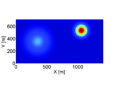
Figure 13: Prior belief map (distribution) for targets.

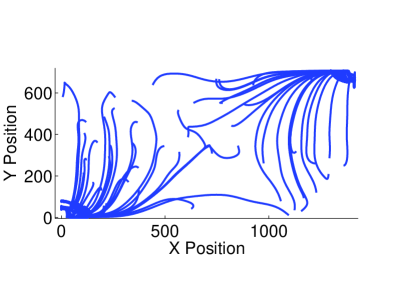
Figure 14: Trajectories generated using distributing spectral search algorithm that uses wave equation based clustering.

8 Conclusions

In this work, we have constructed a wave equation based algorithm for computing the clusters in a graph. The algorithm is completely distributed and at every node one can compute cluster assignments based solely on local information. In addition, this algorithm is orders of magnitude faster than state-of-the-art distributed eigenvector computation algorithms. Starting from a random initial condition at every node, one evolves the wave equation and updates the state based solely on the scalar states of neighbors. One then performs an FFT at each node and computes the sign of the components of the eigenvectors of the graph Laplacian. Complete eigenvector information can be transmitted to each node using multi-hop communication. This process is equivalent to spectral clustering.

The algorithm is also attractive from a distributed computing point of view, where parallel simulations of large dynamical systems [50] can be coupled to the distributed clustering approach presented here, to provide scalable solutions for problems that are computationally and theoretically intractable. This application is the subject of current research.

Wave equation based clustering is demonstrated on community detection examples. Applications to multi-scale distributed estimation and distributed search are also demonstrated.

Current work includes the extension of the wave equation based algorithm for dynamic networks. This is clearly very important in situations where the weights on the edges of the graph are time varying. Examples of systems where dynamic graphs arise include UAV swarms, nonlinear dynamical systems and evolving social graphs.

References

- [1] F. R. K. Chung, Spectral Graph Theory, 1st ed. American Mathematical Society, 1997.
- [2] U. von Luxburg, “A tutorial on spectral clustering,” Statistics and Computing, vol. 17, pp. 395–416, 2007.
- [3] M. Fiedler, “Algebraic connectivity of graphs,” Czechoslovak Mathematical Journal, vol. 23, pp. 289–305, 1973.
- [4] ——, “A property of eigenvectors of nonnegative symmetric matrices and its application to graph theory,” Czechoslovak Mathematical Journal, vol. 25, no. 4, pp. 619–633, 1975.
- [5] C. P. Kottak, Cultural Anthropology, 5th ed. McGraw-Hill, 1991.
- [6] N. Speer, H. Fröhlich, C. Spieth, and A. Zell, “Functional grouping of genes using spectral clustering and gene ontology,” IEEE International Joint Conference on Neural Networks, vol. 1, pp. 298–303, 2005.
- [7] A. Paccanaro, J. A. Casbon, and M. A. S. Saqi, “Spectral clustering of protein sequences,” Nucleic Acid Research, vol. 34, pp. 1571–1580, 2006.
- [8] I. F. Akyildiz, W. Su, Y. Sankarasubramaniam, and E. Cayirci, “A survey on sensor networks,” IEEE Communications Magazine, vol. 40, no. 8, pp. 102–114, 2002.
- [9] S. Ghiasi, A. Srivastava, X. Yang, and M. Sarrafzadeh, “Optimal energy aware clustering in sensor networks,” Sensors, vol. 2, pp. 258–269, 2002.
- [10] A. Muhammad and A. Jadbabaie, “Distributed computation of homology groups by gossip,” in Proceedings of the American Control Conference, 2007, pp. 3438–3443.
- [11] I. Herman, G. Melançon, and M. S. Marshall, “Graph visualization and navigation in information visualization: A survey,” IEEE Transactions on Visualization and Computer Graphics, vol. 6, no. 1, pp. 24–43, 2000.
- [12] D. Kempe and F. McSherry, “A decentralized algorithm for spectral analysis,” Journal of Computer and System Sciences, vol. 74, no. 1, pp. 70–83, 2008.
- [13] M. Stoer and F. Wagner, “A simple min-cut algorithm,” Journal of the ACM, vol. 44, no. 4, pp. 585–591, 1997.
- [14] D. Wagner and F. Wagner, “Between min cut and graph bisection,” in Proceedings of the 18th International Symposium on Mathematical Foundations of Computer Science (MFCS), 1993, pp. 744–750.
- [15] M. A. Porter, J.-P. Onnela, and P. J. Mucha, “Communities in networks,” Notices of the American Mathematical Society, 2009.
- [16] B. W. Kernighan and S. Lin, “A efficient heuristic procedure for partitioning graphs,” The Bell System Technical Journal, vol. 49, pp. 291–307, 1970.
- [17] J. Reichardt and S. Burnholdt, “Detecting fuzzy community structures with a Potts model,” Physical Review Letters, vol. 93, p. 218701, 2004.
- [18] G. Palla, I. Derényi, I. Farkas, and T. Vicsek, “Uncovering the overlapping community structure of complex networks in nature and sociey,” Nature, vol. 435, pp. 814–818, 2005.
- [19] S. Varigonda, T. Kalmar-Nagy, B. Labarre, and I. Mezic, “Graph decomposition methods for uncertainty propagation in complex, nonlinear interconnected dynamical systems,” IEEE Conference on Decision and Control, vol. 2, pp. 1794–1798, 2004.
- [20] D. A. Spielman and S.-H. Teng, “Nearly-linear time algorithms for graph partitioning, graph sparsification, and solving linear systems,” in Proceedings of the thirty-sixth annual ACM symposium on Theory of computing, 2004, pp. 81–90.
- [21] G. Golub and C. V. Loan, Matrix Computations. John Hopkins University Press, 1996.
- [22] M. Kac, “Can one hear the shape of a drum?” The American Mathematical Monthly, vol. 73, no. 4, pp. 1–23, 1966.
- [23] B. Mohar, “The Laplacian spectrum of graphs,” Department of Mathematics, Simon Fraser University, Canada, Tech. Rep., 1991.
- [24] U. v. Luxburg, O. Bousquet, and M. Belkin, “On the convergence of spectral clustering on random samples: the normalized case,” in Proceedings of the 17th Annual Conference on Learning Theory (COLT), 2004, pp. 457–471.
- [25] D. Shah, Gossip Algorithms. Now Publisher Inc., 2009.
- [26] L. C. Evans, Partial Differential Equations. American Mathematical Society, 1998.
- [27] M. Hein, “Uniform convergence of adaptive graph-based regularization,” in Proceedings of the 19th Annual Conference on Learning Theory. Springer, 2006, pp. 50–64.
- [28] M. Hein, J.-Y. Audibert, and U. von Luxburg, “From graphs to manifolds - weak and strong pointwise consistency of graph Laplacians,” in Proceedings of the 18th Annual Conference on Learning Theory. Springer, 2005, pp. 470–485.
- [29] M. Belkin and P. Niyogi, “Towards a theoretical foundation for Laplacian-based manifold methods,” Journal of Computer and System Sciences, vol. 74, pp. 1289–1308, 2008.
- [30] B. Nadler, S. Lafon, R. R. Coifman, and I. G. Kevrekidis, “Diffusion maps, spectral clustering and eigenfunctions of Fokker-Planck operators,” Advances in Neural Information Processing Systems, vol. 18, 2006.
- [31] ——, “Diffusion maps, spectral clustering and reaction coordinates of dynamical systems,” Applied and Computational Harmonic Analysis: Special Issue on Diffusion Maps and Wavelets, vol. 21, pp. 113 –127, 2006.
- [32] M. Franceschelli, A. Gasparri, and A. G. C. Seatzu, “Decentralized Laplacian eigenvalues estimation for networked multi-agent systems,” Proceedings of the Conference on Decision and Control, 2009.
- [33] J. Friedman and J. P. Tillich, “Wave equations for graphs and edge-based Laplacians,” Pacific Journal of Mathematics, vol. 216, no. 2, pp. 229–266, 2004.
- [34] R. R. Coifman, Y. Shkolnisky, F. J. Sigworth, and A. Singer, “Graph Laplacian tomography from unknown random projections,” IEEE Transactions on Image Processing, vol. 17, no. 10, pp. 1891–1899, 2008.
- [35] R. O. Schmidt, “Multiple emitter location and signal parameter estimation,” IEEE Transactions on Antennas and Propagation, vol. AP-34, no. 3, pp. 276–280, 1986.
- [36] S. Boyd, P. Diaconis, and L. Xiao, “Fastest mixing Markov chain on a graph,” SIAM Review, vol. 46, pp. 667–689, 2004.
- [37] W. W. Zachary, “An information flow model for conflict and fission in small groups,” Journal of Anthropological Research, vol. 33, pp. 452–473, 1977.
- [38] A. Lancichinetti, S. Fortunato, and F. Radicchi, “Benchmark graphs for testing community detection algorithms,” Physical Review E, vol. 78, p. 046110, 2008.
- [39] M. Girvan and M. E. J. Newman, “Community structure in social and biological networks,” Proceedings of the National Academy of Sciences, vol. 99, no. 12, pp. 7821–7826, 2002.
- [40] M. E. J. Newman, “Modularity and community structure in networks,” Proceedings of the National Academy of Sciences, vol. 103, pp. 8577–8582, 2006.
- [41] M. Rosvall and C. T. Bergstrom, “An information-theoretic framework for resolving community structure in complex networks,” Proceedings of the National Academy of Sciences, vol. 104, no. 18, pp. 7327–7331, 2007.
- [42] P. Alrikson and A. Rantzer, “Experimental evaluation of a distributed Kalman filter algorithm,” in IEEE Conference on Decision and Control, 2007.
- [43] R. Olfati-Saber, “Distributed Kalman filtering for sensor networks,” in IEEE Conference on Decision and Control, 2007.
- [44] R. Carli, A. Chiuso, L. Schenato, and S. Zampieri, “Distributed Kalman filtering based on consensus strategies,” IEEE Journal on Selected Areas in Communications, vol. 26, pp. 622–633, 2008.
- [45] A. Speranzon, C. Fischione, K. H. Johansson, and A. Sangiovanni-Vincentelli, “A distributed minimum variance estimator for sensor networks,” IEEE Journal on Selected Areas in Communications, vol. 26, pp. 609–621, 2008.
- [46] J.-H. Kim, M. West, E. Scholte, and S. Narayanan, “Multiscale consensus for decentralized estimation and its application to building systems,” in American Control Conference, 2008.
- [47] J.-H. Kim, M. West, S. Lall, E. Scholte, and A. Banaszuk, “Stochastic multiscale approaches to consensus problems,” in Conference on Decision and Control, 2008.
- [48] C. Selle and M. West, “Multiscale networks for distributed consensus algorithms,” in IEEE Conference on Decision and Control and Chinese Control Conference, 2009.
- [49] G. Mathew and I. Mezic, “Spectral multiscale coverage: A uniform coverage algorithm for mobile sensor networks,” in Proceedings of the Conference on Decision and Control, 2009, pp. 7872–7877.
- [50] S. Klus, T. Sahai, C. Liu, and M. Dellnitz, “An efficient algorithm for the parallel solution of high-dimensional differential equations,” Journal of Computational and Applied Mathematics, vol. 235, no. 9, pp. 3053–3062, 2011.