Abstract

The probability of emission of a single photon via Raman scattering of laser pulse on the three-level $\Lambda$ - type atom in microcavity is studied. The duration of the pulse is considered to be short enough, so that the hyperfine structure of the upper level remains totally unresolved, while that of the lower level is totally resolved. The coherent laser pulse is assumed to be in resonance with the transition between one hyperfine structure component of the lower atomic level and all hyperfine structure components of the upper level, while the quantized cavity field is assumed to be in resonance with the transition between the other hyperfine structure component of the lower level and all components of the upper one. The dependence of the photon emission probability on the mutual orientation of polarization vectors of the cavity mode and of the coherent laser pulse is analyzed. Particularly, the case is investigated, when the total electronic angular momentum of the lower atomic level equals 1/2, which is true for the ground states of alkali atoms employed in the experiments on deterministic single photon emission. It is shown, that in this case the probability of photon emission equals zero for collinear polarizations of the photon and of the laser pulse, and the probability obtains its maximum value, when the angle between their polarizations equals $60^{\circ}$.

1 Introduction

The implementation of quantum optical devices for quantum information processing is a rapidly developing field of research nowadays, passing the threshold from a learning phase into a domain of rudimentary functionality [1]. Among such devices the three-level $\Lambda$ - type atom placed inside a high-finesse cavity proved to be a useful building block for quantum communication schemes because of its ability to interface efficiently atoms and photons [2, 3, 4]. As it was pointed out in [5] and then realized experimentally in [6, 7, 8], such atoms may be employed for the controlled generation of a single photon in the cavity by means of vacuum-stimulated Raman scattering. In these experiments one branch of the atomic $\Lambda$ - type transitions was coupled to the quantized cavity field, while the other one was coupled to the coherent laser field. In course of resonant interaction with the fields inside the cavity the atom emitted a single photon. The effectiveness of this process depends on the interaction parameters, in particular, it depends on the relative orientation of polarizations of the cavity field and of the laser field, since the atomic levels are usually strongly degenerate and the contributions of various Zeeman components of resonant levels to the interaction are determined by the polarizations of the fields. Thus in the experiment [3, 4] the transitions between hyperfine components $F_{a}=3$ and $F^{\prime}_{a}=4$ of the ground state $6S_{1/2}$ and the component $F_{b}=4$ of the excited state $6P_{3/2}$ of Cesium atoms were employed, while in the experiments [6, 7, 8] they were the transitions between hyperfine components $F_{a}=2$ and $F^{\prime}_{a}=3$ of the ground state $5S_{1/2}$ and the component $F_{b}=3$ of the excited state $5P_{3/2}$ of Rubidium atoms. Such polarization dependencies were studied previously [9] for rather long interaction times, when the hyperfine structure of both the ground and the excited states was totally resolved. In this paper we study the polarization dependencies of the probability of single-photon emission via Raman scattering of rather short coherent laser pulses, such that the hyperfine structure of the excited level appears to be totally unresolved. However we consider the hyperfine structure of the ground state to remain totally resolved, since the frequencies of hyperfine splitting of ground states of alkali atoms are significantly greater, than those of the excited states. In section 2 we describe the interaction model and obtain the evolution operator for this model, while in section 3 we obtain the expression for the probability of single photon emission and analyze it numerically for the transitions in Cesium and Rubidium, employed in the experiments [3, 4] and [6, 7, 8].

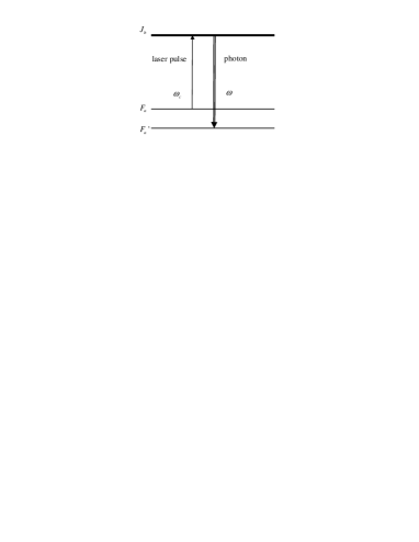
Figure 1: The level diagram.

2 Evolution operator

We assume, that the coherent laser pulse with the carrier frequency $\omega_{c}$ is in resonance with the transition $F_{a}\rightarrow J_{b}$ between one hyperfine structure component $F_{a}$ of the ground state $a$ and all the hyperfine structure components $F_{b}$ of the excited state $b$, while the quantized cavity field with the carrier frequency $\omega$ is in resonance with the transition $F^{\prime}_{a}\rightarrow J_{b}$ between some other hyperfine structure component $F^{\prime}_{a}$ of the ground state and all the components of the excited state (Fig.1). Here $F_{a}$ and $F_{b}$ are the values of the atomic total angular momenta of the ground and excited states respectively, while $J_{a}$ and $J_{b}$ denote electronic total angular momenta of these states, $F_{a,b}=|J_{a,b}-I|,...,J_{a,b}+I$, $I$ being the value of nuclear spin. The electric field strength, which contains the coherent field of the pulse and the quantized field of the cavity, may be put down as:

$${\bf\hat{E}\/}=e_{c}{\bf l\/}_{c}e^{-\imath\omega_{c}t}+\imath e_{0}{\bf l\/}\hat{a}e^{-\imath\omega t}+h.c.~{},$$ (1)

where $e_{c}$ and ${\bf l\/}_{c}$ are the constant amplitude and the unit polarization vector of the pulse, $\hat{a}$ is the photon annihilation operator for the cavity mode, while

$$e_{0}=\sqrt{\frac{2\pi\hbar\omega}{V_{c}}},$$ (2)

is the photon field, $V_{c}$ being the cavity (quantization) volume, ${\bf l\/}$ - the unit polarization vector of the cavity field. The quantum system consists of the atom and of the quantized field. The equation for the slowly-varying density matrix $\hat{\rho}$ of this system in the rotating-wave approximation is as follows:

$$\dot{\hat{\rho}}=\imath\left[\hat{V},\hat{\rho}\right],~{}\hat{V}=\chi_{c}\hat{p}_{c}-\imath\chi\hat{p}\hat{a}^{+}+h.c.$$ (3)

Here $\chi_{c}=|d|e_{c}/\hbar$ and $\chi=|d|e_{0}/\hbar$ are the reduced Rabi frequencies for the coherent pulse and for the cavity field, $d=d(J_{a}J_{b})$ being the reduced matrix element of the electric dipole moment operator for the electronic transition $J_{a}\rightarrow J_{b}$, while

$$\hat{p}_{c}=\hat{\textbf{g}}_{c}\textbf{l}_{c}^{*},~{}\hat{p}=\hat{\textbf{g}}\textbf{l}^{*},$$ (4)

$\hat{\textbf{g}}_{c}$ and $\hat{\textbf{g}}$ are the dimensionless electric dipole moment operators for the transitions $F_{a}\rightarrow J_{b}$ and $F^{\prime}_{a}\rightarrow J_{b}$. The circular components of these vector operators are expressed through Wigner 3J- and 6J- symbols and partial operators

$$\hat{P}^{F_{\alpha}F^{\prime}_{\beta}}_{M_{\alpha}M^{\prime}_{\beta}}=|F_{\alpha}M_{\alpha}><F^{\prime}_{\beta}M^{\prime}_{\beta}|,~{}\alpha,\beta=a,b,$$ (5)

in a following way:

$$\hat{g}_{cq}=\sum_{M_{a},M_{b},F_{b}}(g_{cq})^{F_{a}F_{b}}_{M_{a}M_{b}}\cdot\hat{P}^{F_{a}F_{b}}_{M_{a}M_{b}},$$ (6)

$$\hat{g}_{q}=\sum_{M^{\prime}_{a},M_{b},F_{b}}(g_{q})^{F^{\prime}_{a}F_{b}}_{M^{\prime}_{a}M_{b}}\cdot\hat{P}^{F^{\prime}_{a}F_{b}}_{M^{\prime}_{a}M_{b}},$$ (7)

$$(g_{cq})^{F_{a}F_{b}}_{M_{a}M_{b}}=(-1)^{F_{a}-M_{a}}\left(\matrix{F_{a}&1&F_{b}\cr-M_{a}&q&M_{b}}\right)g_{F_{a}F_{b}},$$ (8)

$$(g_{q})^{F^{\prime}_{a}F_{b}}_{M^{\prime}_{a}M_{b}}=(-1)^{F^{\prime}_{a}-M^{\prime}_{a}}\left(\matrix{F^{\prime}_{a}&1&F_{b}\cr-M^{\prime}_{a}&q&M_{b}}\right)g_{F^{\prime}_{a}F_{b}},$$ (9)

$$g_{F_{a}F_{b}}=(-1)^{F_{a}+J_{a}+I+1}G_{F_{a}F_{b}},$$ (10)

$$G_{F_{a}F_{b}}=[(2F_{a}+1)(2F_{b}+1)]^{1/2}\left\{\matrix{I&F_{a}&J_{a}\cr 1&J_{b}&F_{b}}\right\}.$$ (11)

Note, that the summation in (6) and (7) is carried out over all possible values of the atomic total angular momentum $F_{b}$ of the excited state.

After the action of the coherent pulse with the duration $T$ the system density matrix, being initially $\hat{\rho}_{0}$, evolves to:

$$\hat{\rho}=\hat{S}\hat{\rho}_{0}\hat{S}^{+},$$ (12)

where the evolution operator $\hat{S}$ may be expressed through the matrix exponent:

$$\hat{S}=\exp\left(\imath\hat{V}T\right)=\exp\left\{\imath\left(\hat{G}+\hat{G}^{+}\right)\right\},$$ (13)

$$\hat{G}=\theta_{c}\hat{p}_{c}-\imath\theta\hat{a}^{+}\hat{p},~{}\theta_{c}=\chi_{c}T,~{}\theta=\chi T.$$ (14)

With the use of the expansion of the exponent function in Taylor series and with the use of relation

$$(\hat{G}+\hat{G}^{+})^{2n}=\hat{Q}^{2n}+\hat{G}\hat{Q}^{2(n-1)}\hat{G}^{+}~{},~{}n=1,2,...~{},$$ (15)

where

$$\hat{Q}^{2}=\theta^{2}_{c}\hat{p}_{c}^{+}\hat{p}_{c}+\theta^{2}\hat{a}\hat{a}^{+}\hat{p}^{+}\hat{p},$$ (16)

the evolution operator $\hat{S}$ may be transformed to the expression:

$$\hat{S}=\hat{P}_{F_{a}}+\hat{P}_{F^{\prime}_{a}}+\hat{C}-\frac{1}{2}\hat{G}\hat{F}\hat{G}^{+}+\imath\hat{G}\hat{H}+\imath\hat{H}\hat{G}^{+},$$ (17)

$$\hat{C}=\cos(\hat{Q}),~{}\hat{H}=\frac{\sin(\hat{Q})}{\hat{Q}},~{}\hat{F}=\frac{\sin^{2}(\hat{Q}/2)}{(\hat{Q}/2)^{2}}.$$ (18)

3 The probability of single-photon emission

Initially the atom is at the equilibrium ground state, while the cavity field is at the vacuum state, so that the initial system density matrix is:

$$\hat{\rho}_{0}=\frac{1}{2F_{a}+1}\hat{P}_{F_{a}}\cdot|0><0|,$$ (19)

$\hat{P}_{F_{a}}$ being the projector on the subspace of the hyperfine-structure component $F_{a}$. The probability to detect a single photon in the cavity is given by the formula:

$$w=Tr\{<1|\hat{\rho}|1>\},$$ (20)

where the trace is carried out in atomic variables. With the use of the evolution operator (17) this probability may be written as:

$$w=\frac{1}{(2F_{a}+1)}Tr\{\hat{R}\hat{R}^{+}\},$$ (21)

with

$$\hat{R}=\frac{\theta\theta_{c}}{2}\hat{p}\frac{\sin^{2}(\hat{Q}_{b}/2)}{(\hat{Q}_{b}/2)^{2}}\hat{p}_{c}^{+},$$ (22)

while the atomic operator

$$\hat{Q}_{b}^{2}=\theta^{2}_{c}\hat{p}_{c}^{+}\hat{p}_{c}+\theta^{2}\hat{p}^{+}\hat{p}$$ (23)

acts in the subspace of the excited level $b$. The operators $\hat{R}$ in (21) may be also expressed in terms of atomic operators

$$\hat{Q}_{a}^{2}=\theta^{2}_{c}\hat{p}_{c}\hat{p}_{c}^{+}+\theta^{2}\hat{p}\hat{p}^{+}+\theta\theta_{c}(\hat{p}\hat{p}_{c}^{+}+\hat{p}_{c}\hat{p}^{+}),$$ (24)

acting in the subspace of the ground state levels $F_{a}$ and $F^{\prime}_{a}$:

$$\hat{R}=\hat{P}_{F^{\prime}_{a}}\cos(\hat{Q}_{a})\hat{P}_{F_{a}},$$ (25)

since

$$\theta\theta_{c}\hat{p}\hat{Q}_{b}^{2n}\hat{p}_{c}^{+}=\hat{P}_{F^{\prime}_{a}}\hat{Q}_{a}^{2(n+1)}\hat{P}_{F_{a}},~{}n=0,1,2...$$ (26)

The presentation of operators $\hat{R}$ in (21) by means of $\hat{Q}_{a}$ is more convenient here, than by means of $\hat{Q}_{b}$, because the summation in (24) in all possible values of the total angular momenta $F_{b}$ of the upper level and its projections $M_{b}$ may be carried out analytically with the help of the summation formulae for 3J- and 6J-symbols [10]. After such summation the operator $\hat{Q}_{a}^{2}$ (24) becomes as follows:

$$\hat{Q}_{a}^{2}=\theta^{2}_{c}\hat{A}_{c}+\theta^{2}\hat{A}+\theta\theta_{c}(\hat{B}+\hat{B}^{+}),$$ (27)

$$\hat{A}_{c}=\sum_{M_{a},M^{\prime}_{a}}(A_{c})^{F_{a}F_{a}}_{M_{a}M^{\prime}_{a}}\cdot\hat{P}^{F_{a}F_{a}}_{M_{a}M^{\prime}_{a}},$$ (28)

$$\hat{A}=\sum_{M_{a},M^{\prime}_{a}}(A)^{F^{\prime}_{a}F^{\prime}_{a}}_{M_{a}M^{\prime}_{a}}\cdot\hat{P}^{F^{\prime}_{a}F^{\prime}_{a}}_{M_{a}M^{\prime}_{a}},$$ (29)

$$\hat{B}=\sum_{M_{a},M^{\prime}_{a}}(B)^{F_{a}F^{\prime}_{a}}_{M_{a}M^{\prime}_{a}}\cdot\hat{P}^{F_{a}F^{\prime}_{a}}_{M_{a}M^{\prime}_{a}},~{}$$ (30)

$$(B)^{F_{a}F^{\prime}_{a}}_{M_{a}M^{\prime}_{a}}=(-1)^{M^{\prime}_{a}}\sum_{k,q}\left(\matrix{k&F_{a}&F^{\prime}_{a}\cr q&M_{a}&-M^{\prime}_{a}}\right)a_{k}f^{k}_{q},$$ (31)

$$a_{k}=(-1)^{F^{\prime}_{a}-F_{a}+I-J_{b}}(2k+1)\left\{\matrix{k&1&1\cr J_{b}&J_{a}&J_{a}}\right\}b_{k},$$ (32)

$$b_{k}=[(2F_{a}+1)(2F^{\prime}_{a}+1)]^{1/2}\left\{\matrix{k&F_{a}&F^{\prime}_{a}\cr I&J_{a}&J_{a}}\right\},$$ (33)

$$f^{k}_{q}=\sum_{q_{1},q_{2}}(-1)^{q}(l_{c})_{-q_{1}}(l)_{-q_{2}}\left(\matrix{k&1&1\cr q&q_{1}&q_{2}}\right).$$ (34)

The matrix elements $(A)^{F^{\prime}_{a}F^{\prime}_{a}}_{M_{a}M^{\prime}_{a}}$ are obtained from $(B)^{F_{a}F^{\prime}_{a}}_{M_{a}M^{\prime}_{a}}$ by the substitutions $A\rightarrow B$, $F^{\prime}_{a}\rightarrow F_{a}$ elsewhere in (31)-(33) and $l\rightarrow l_{c}$ in (34), while elements $(A_{c})^{F_{a}F_{a}}_{M_{a}M^{\prime}_{a}}$ are obtained from $(B)^{F_{a}F^{\prime}_{a}}_{M_{a}M^{\prime}_{a}}$ by the substitutions $A_{c}\rightarrow B$, $F_{a}\rightarrow F^{\prime}_{a}$ in (31)-(33) and $l_{c}\rightarrow l$ in (34). Now the probability (21) may be calculated by reducing the hermitian $2(F_{a}+F^{\prime}_{a}+1)\times 2(F_{a}+F^{\prime}_{a}+1)$ matrix $Q_{a}$ to its diagonal form.

Figure 2: Probability $w$ of single photon emission versus reduced Rabi angle $\theta$ = $\theta_{c}$ at the orthogonal polarizations $\psi=90^{\circ}$ of the cavity and laser fields. Solid line refers to the angular momenta $F_{a}=2$, $F^{\prime}_{a}=3$, $I=5/2$, $J_{a}=1/2$, $J_{b}=3/2$, while the dashed line refers to $F_{a}=3$, $F^{\prime}_{a}=4$, $I=7/2$, $J_{a}=1/2$, $J_{b}=3/2$.

The matrices $\hat{A}$, $\hat{A}_{c}$ and $\hat{B}$ in (27) simplify essentially in case, when the electronic angular momentum of the atomic ground state equals $1/2$: $J_{a}=1/2$, which is the usual case for alkali metals. In this case we obtain:

$$\hat{A}_{c}=\frac{1}{6}\hat{P}_{F_{a}},~{}\hat{A}=\frac{1}{6}\hat{P}_{F^{\prime}_{a}},$$

$$(B)^{F_{a}F^{\prime}_{a}}_{M_{a}M^{\prime}_{a}}=\imath\sin(\psi)\delta_{M_{a},M^{\prime}_{a}}B(F_{a},F^{\prime}_{a},M_{a}),$$

where $\psi$ is the angle between polarization vectors of the coherent pulse ${\bf l_{c}}$ and of the cavity field ${\bf l}$, while functions $B(F_{a},F^{\prime}_{a},M_{a})$ are defined from (31)-(34). So, in this case the photon will not be emitted in the cavity $w=0$, if the polarizations of the coherent pulse and of the photon are collinear: $\psi=0$. The dependence of the probability $w$ of single photon emission on the reduced vacuum Rabi angle $\theta$ of the cavity field, which is considered to be equal to the reduced area $\theta_{c}$ of the coherent laser pulse ($\theta$=$\theta_{c}$), at the orthogonal polarizations $\psi=90^{\circ}$ of the cavity and laser fields is presented at Fig.2. The solid line refers to the values of the angular momenta $F_{a}=2$, $F^{\prime}_{a}=3$, $I=5/2$, $J_{a}=1/2$, $J_{b}=3/2$ corresponding to the transitions in ${}^{85}Rb$, while the dashed line refers to $F_{a}=3$, $F^{\prime}_{a}=4$, $I=7/2$, $J_{a}=1/2$, $J_{b}=3/2$ corresponding to the transitions in ${}^{133}Cs$. In both cases the maximum probability values are obtained at the same value of Rabi angles $\theta_{max}=19.604$, though the values of probability at $\theta=\theta_{max}$ slightly differ: $w_{max}=0.8943$ for Rubidium transitions and $w_{max}=0.8855$ for Cesium transitions. The greater probabilities are obtained, if the coherent laser pulse in course of photon emission drives the atom from the less degenerate hyperfine structure component $F_{a}$ to the more degenerate one $F^{\prime}_{a}>F_{a}$, otherwise the probabilities are decreased by the factor $(2F_{a}+1)/(2F^{\prime}_{a}+1)$. However the maximum emission probabilities occur not at the orthogonal polarizations of laser and cavity fields. The Fig.3 represents the dependence of the probability $w$ of single photon emission at Rabi angle $\theta$=$\theta_{c}$=$\theta_{max}=19.604$, corresponding to the maximum probability values, on the angle $\psi$ between polarization vectors of the laser pulse and of the cavity field. The solid line, like at Fig.2, refers to Rubidium transitions with $F_{a}=2$, $F^{\prime}_{a}=3$, $I=5/2$, $J_{a}=1/2$, $J_{b}=3/2$, while the dashed line refers to Cesium transitions with $F_{a}=3$, $F^{\prime}_{a}=4$, $I=7/2$, $J_{a}=1/2$, $J_{b}=3/2$. As it may be seen from Fig.3 the maximum probabilities of the photon emission are obtained at the angle $\psi=60^{\circ}$ and the maximum probability values are: $w_{max}=0.9595$ for Rubidium transitions and $w_{max}=0.9397$ for Cesium transitions.

Figure 3: Probability $w$ of single photon emission versus angle $\psi$ between polarization vectors of the laser pulse and of the cavity field at the reduced Rabi angle $\theta$=$\theta_{c}$=$\theta_{max}=19.604$. Solid line refers to the angular momenta $F_{a}=2$, $F^{\prime}_{a}=3$, $I=5/2$, $J_{a}=1/2$, $J_{b}=3/2$, while the dashed line refers to $F_{a}=3$, $F^{\prime}_{a}=4$, $I=7/2$, $J_{a}=1/2$, $J_{b}=3/2$.

4 Conclusions

In the present paper we derived the expression for the probability of single photon emission via Raman scattering of short laser pulse under the conditions when the hyperfine structure of the atomic ground state is totally resolved, while the the hyperfine structure of the excited state is totally unresolved, for arbitrary values of the level angular momenta. In case of the ground state electronic angular momentum $J_{a}=1/2$, which is the usual case for the experiments on deterministic single photon emission in alkali metals, the emission probability strongly depends on the angle between polarizations of the laser pulse and of the quantized cavity field - this probability is zero at the collinear polarizations of the cavity and laser fields and it obtains its maximum values close to unity, when the angle between their polarizations constitutes $60^{\circ}$. The greater emission probabilities are obtained, if the coherent laser pulse drives the atom from the less degenerate hyperfine structure component to the more degenerate one in course of photon emission.

Acknowledgements

Authors are indebted for financial support of this work to Russian Foundation for Basic Research (grant 08-02-00161).

References

• [1] H.J. Kimble, Nature 453 (2008), pp. 1023-1030.
• [2] A.V. Gorshkov, A. Andre, M. Fleischhauer, A.S. Sorensen and M.D. Lukin, Phys.Rev.Lett. 98 (2007), 123601.
• [3] J. Laurat, H. Riedmatten, D. Felinto, Ch. Chou, E. Scomburg and H.J. Kimble, Opt.Express 14 (2006), pp. 6912-6918.
• [4] J. Laurat, K.S. Choi, H. Deng, C. Chou and H.J. Kimble, Phys.Rev.Lett. 99 (2007), 180504.
• [5] A.S. Parkins, P. Marte, P. Zoller and H.J. Kimble, Phys.Rev.Lett. 71 (1993), pp. 3095-3098.
• [6] M. Hennrich, T. Legero, A. Kuhn and G. Rempe, Phys.Rev.Lett. 85 (2000), pp. 4872-4875.
• [7] A. Kuhn, M. Hennrich and G. Rempe, Phys.Rev.Lett. 89 (2002), 067901.
• [8] T. Wilk, S.C. Webster, H.P. Specht, G. Rempe and A. Kuhn, Phys.Rev.Lett. 98 (2007), 063601.
• [9] V.A. Reshetov and I.V. Yevseyev, Laser Phys.Lett. 5 (2008), pp. 608-613.
• [10] I.I. Sobelman, Introduction to the Theory of Atomic Spectra, Pergamon, New York (1972).