Tracing High Redshift Starformation in the Current and Next Generation of Radio Surveys

Abstract:

The current deepest radio surveys detect hundreds of sources per square degree below $0.1\,$mJy. There is a growing consensus that a large fraction of these sources are dominated by star formation although the exact proportion has been debated in the literature. However, the low luminosity of these galaxies at most other wavelengths makes determining the nature of individual sources difficult. If future, deeper surveys performed with the next generation of radio instrumentation are to reap high scientific reward we need to develop reliable methods of distinguishing between radio emission powered by active galactic nuclei (AGN) and that powered by star formation. In particular, we believe that such discriminations should be based on purely radio, or relative to radio, diagnostics. These diagnostics include radio morphology, radio spectral index, polarisation, variability, radio luminosity and flux density ratios with non-radio wavelengths e.g. with different parts of the infrared (IR) regime. We discuss the advantages and limitations of these various diagnostics methods with current and future surveys. However, weeding AGN out of deep radio surveys can already provide several insights into the star formation at high redshift. As well as reproducing the well known rise with redshift in the comoving star formation rate density, we also see evidence for the continued dominance of LIRGs and ULIRGs to the total star forming budget across redshifts $1-3$. Additionally, while we see that the IR-radio relation for star forming galaxies does hold to high redshifts ($z>1$) there is a mild deviation depending on the IR waveband used and the range of IR SEDs found. We will discuss the possible reasons behind this change in properties.

1 Introduction

Traditionally radio surveys have been dominated by powerful radio-loud active galactic nuclei (AGN) and radio galaxies were the first probe of the distant Universe [1], and references therein. However, surveys by the next generation of radio telescopes we will obtain vast samples of star forming galaxies (SFGs). In fact, as studies of star formation, these surveys will have several advantages over current surveys at other wavelengths. Firstly, radio luminosity is a direct tracer of star formation rate (SFR) once AGN activity has been accounted for and secondly, the combination of area and the sensitivity will provide a fast survey speed allowing for an unprecedented census of star formation in the distant Universe.

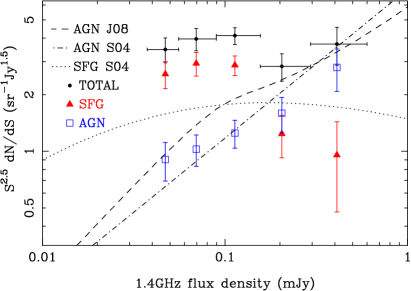
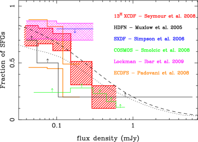
Figure 1: Left The $1.4\,$GHz Euclidean normalised source counts from the $13^{\rm H}$ field divided into SFGs and AGN [2]. Models of the contribution from different populations are overlaid: S04 [3], J08 [4]. Right Compilation from the literature of the fraction of SFGs as a function of $1.4\,$GHz flux density [2,5,6,7,8,9].

The sub-mJy regime of the radio source counts has been studied for several decades now and the up-turn below $\sim 1\,$mJy has been well characterised albeit with some scatter. Currently the debate is over the normalisation of the source counts and type of sources that are responsible for the up-turn. However, the most important question is how do we distinguish between AGN and SFGs in the deepest surveys?

We believe that as some AGN have very low emission in the radio, compared to even low Milky Way rates of star formation, the simple presence of an AGN does not necessarily infer that the radio emission of a galaxy is from an accretion driven source. Hence, methods to discriminate between whether AGN or star forming activity contribute to the observed radio flux density should be related to the radio emission, and we list some of these methods here:

• Radio morphology

• Radio spectral index/radio Spectral Energy Distribution (SED)

• Radio variability

• Radio polarisation

• Flux density ratios/full SED modeling

This list is not exhaustive and several of these methods have already been used in various combinations (e.g. [2,5,6,7,8,9]). We have found that a combination of the radio morphology and spectral index is the most effective method if you have data of sufficient quality, but in practice for the deepest surveys the flux ratio method, based on SEDs of SFGs and AGN, is the most productive. So employing these techniques, and on the assumption that one process dominates we can separate the faint radio source counts by galaxy type (e.g. Fig. 1 left).

We have demonstrated that while AGN dominate the 1.4 GHz source counts around 0.4 mJy, SFGs make up $70-80\%$ below 0.1 mJy [2] with the transition between the two populations occuring between $0.1$ and $0.2\,$mJy. So while SFGs dominate at the faintest flux densities there remains a non-negligible contribution from radio quiet AGN around $50\,\mu$Jy. This result is consistent with determinations and constraints in the literature (Fig. 1 right) which are reaching a consensus about the nature of the faint radio source counts. The observed differences in this plot are easily explained by the different methods used in discriminating between AGN and SFGs as well as sample variance between the different deep narrow survey fields used in each study.

Our knowledge of the faint radio source population will be greatly improved with surveys from up-coming radio facilities (see other contributions to these proceedings). At fainter flux densities the modeled evolution of the luminosity function of both populations suggests that the fraction of SFGs will asymptote towards $100\%$ [4]. The eVLA and eMERLIN will push to such flux densities where star formation completely dominates and provide samples of radio-selecting SFGs out to the highest redshifts. Other projects, like the Evolutionary Map of the Universe (EMU, see [10] in these proceedings) on the Australian Square Kilometer Array Pathfinder, will probe the star forming regime well below $0.1\,$mJy over a large fraction of the whole sky. However, in preparation for such surveys we must obtain a better understanding of radio emission from star formation in the local Universe and a better understanding of the radio luminosity to star formation rate (SFR) conversion.

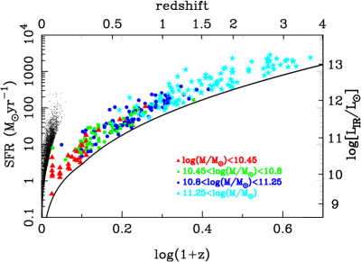
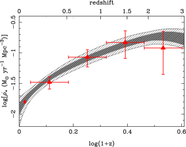
Figure 2: Left Star formation rate plotted against redshift for a sample of radio selected SFGs from the $13^{\rm H}$ field (coloured symbols indicating host galaxies of different stellar masses). Local radio-selected star forming galaxies are illustrated by black dots. Equivalent IR luminosity is plotted on the right axis. At high redshift we see massive galaxies with star formation rates in excess of that seen in the local Universe. Right Derived comoving star formation rate density (SFRD) as a function of redshift compared with the mean SFRD presented in [11]. The results in the radio agree well with those at other wavelengths which bodes well for future radio surveys making detailed studies of star formation at high redshift.

2 Science with Radio Selected Star Forming Galaxies

With the data we have in hand we can already study the properties of host galaxies of powerful starbursts selected at radio wavelengths. We discover above $z=1$ galaxies with high SFRs which are simply not detected in the local Universe (Fig. 2 left), even allowing for volume effects. In the local Universe the most extreme galaxies have SFRs of $\sim 300\,M_{\odot}$yr^-1 whereas at high redshift we see galaxies with SFRs up to almost an order of magnitude greater. Furthermore, we find that such galaxies are always have high stellar masses implying they have already built up a large population of stars [11].

We can also use such samples to study the comoving star formation rate density (SFRD) as a function of redshift (e.g. [12], [13]). We find that the radio selected sample produce results consistent with those from other wavelengths (Fig. 2 right and [11]). The future radio surveys discussed in the previous section will no doubt greatly increase the accuracy with which we can trace the formation of stars in such a plot.

From radio surveys we can not only study when stars formed, but also where. The contribution to the comoving IR luminosity density (a proxy for the SFRD) by galaxies of different IR luminosities changes with redshift [14]. The contribution of luminous IR galaxies (LIRGs, $10^{11}\leq L/L_{\odot}\leq 10^{12}$) and ultra-luminous IR galaxies (ULIRGs, $10^{12}\leq L/L_{\odot}\leq 10^{13}$) increases from $z=0$ to $z=1$. However, this is not surprising as it is a natural result of integrating a rapidly evolving luminosity function.

By exploiting the IR/radio correlation for SFGs we find that results from radio surveys agree well those from the IR and can extend such studies to redshifts greater than unity. In Fig. 3 we see that LIRGs and ULIRGs continue to make a high contribution to the IR luminosity density across $1\leq z\leq 3$. The extreme starbursts, hyper-luminous IR galaxies (HyLIRGs, $L/L_{\odot}\geq 10^{13}$) which are not seen in the local Universe only contribute a few percent to the total star forming budget at $z=2-3$.

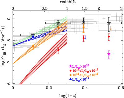
Figure 3: The comoving IR luminosity density (IRLD) plotted as a function of redshift. The gray points are SFRD data converted to IRLD from [15], the shaded regions (from [14]) are the IRLD separated by IR luminosity as indicated in the plot. The coloured points are based on radio-selected SFGs in the $13^{\rm H}$ field and follow the same division by IR luminosity. We observe that the contribution of LIRGs and ULIRGs remains high across $1\leq z\leq 3$.

3 The IR/Radio Relation for Star Forming Galaxies

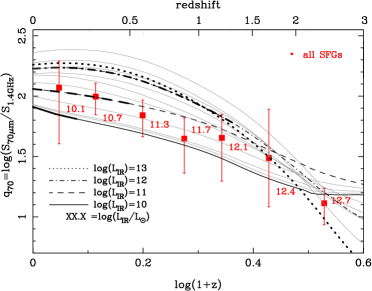
Figure 4: The mean observed value of q₇₀ ($=\log[S_{70\mu m}/S_{1.4GHz}]$) for radio-selected SFGs plotted as a function of redshift (red squares). The numbers beside each data point indicate the mean total IR luminosity derived from the radio SFR. The black lines represent the tracks from local templates from [16] at luminosities of as indicted in the figure. These lines become thinner at the redshift a given template becomes undetectable in our radio survey. The trend of a decrease in q₇₀ toward higher redshifts is generally consistent with the tracks with local SEDs.

An important question for future surveys is does the radio luminosity/star formation rate relation hold at high redshifts and extreme luminosities? This relation primarily depends on the IR/radio correlation. What do we expect at high redshift from local galaxies? In Fig. 4 we show the observed $70\,\mu$m to $1.4\,$GHz flux density ratio for average SEDs of local galaxies [16]. We observe that the flux density ratio increases with IR luminosity which is due to more luminous IR galaxies being characterised by hotter dust temperatures and hence peaking at shorter wavelengths (i.e. they contribute relatively more to the $70\,\mu$m band). However, all the tracks decrease with increasing redshifts due to k-correction effects.

We have stacked $70\,\mu$m images at positions of radio-selected SFGs and hence we can obtain a flux density ratio as a function of redshift, [17] and Fig. 4. We note, however, that we are probing different luminosities at each redshift, hence must be careful to compare each point to the correct SED track. The data broadly agree with the general trend of decreasing flux density ratio toward higher redshift, but there are differences in the detail. We see that the bin at $z\sim 0.9$, which contains SFGs close to ULIRG power ($\bar{L}\sim 10^{11.7}\,L_{\odot}$), lies next to the low luminosity tracks ($\log(L_{IR})=10$) and $2\,\sigma$ away from the ULIRG track. Why might the 70um/radio correlation change at high redshift? Locally the IR SED is luminosity dependent so it is possible that these high redshift luminous starburst may have different IR SEDs compared to local luminous starbursts. If high redshift star forming regions in luminous starbursts are more extended, they may be more optically thin and hence have less free-free absorption (and therefore have a higher radio flux). Such SEDs would also be characterised as being cooler and have a lower $70\,\mu$m flux density.

There is now strong evidence for cold LIRGs and ULIRGs at high redshift. We have found that such galaxies at $0.5\leq z\leq 1.0$ span a range of characteristic dust temperatures from the hot local starbursts to that of higher-z sub-mm selected galaxies [18]. We have also found that luminous galaxies colder than local hot starbursts dominate the luminosity density at these redshifts [19].

4 Conclusions

Radio observations of the distant Universe have traditionally been used to study AGN, but we are now begining to obtain a census of star formation from deep, wide radio surveys. There are three crucial issues in exploiting such data: (i) distinguishing between AGN and SFGs, (ii) calibrating the radio luminosity/SFR relation across all redshifts, radio luminosities and type of galaxy, and (iii) obtaining redshifts from ancillary data. The radio/IR relation for SFGs appears to depend on IR SED and hence waveband used in the IR. We must better understand this relationship locally before applying it to galaxies at high redshift.

References

- [1] G. Miley & C. De Breuck, 2008, A&AR, 15, 67
- [2] N. Seymour et al., 2008, MNRAS, 386, 1695
- [3] N. Seymour et al., 2004, MNRAS, 352, 131
- [4] R. Wilman et al., 2008, MNRAS, 388, 1335
- [5] T. Muxlow et al., 2005, MNRAS, 358, 1159
- [6] C. Simpson et al., 2006, MNRAS, 372, 741
- [7] V. Smolčić et al., 2008, ApJS, 177, 14
- [8] E. Ibar et al., 2008, MNRAS, 386, 953
- [9] P. Padovani et al., 2009, ApJ, 694, 235
- [10] R. Norris et al., 2009, \posPOS(PRA2009)003
- [11] A. Hopkins et al., 2007, ASPC, 380, 423
- [12] S. Lilly et al., 1996, ApJ, 460, L1
- [13] P. Madau et al., 1996, MNRAS, 283, 1388
- [14] E. Le Floc’h et al., 2005, ApJ, 632, 169
- [15] A. Hopkins & J.F. Beacom, 2006, ApJ, 651, 142
- [16] G. Rieke et al., 2009, ApJ, 692, 556
- [17] N. Seymour et al., 2009a, MNRAS, 398, 1573
- [18] M. Symeonidis et al., 2009, MNRAS, 397, 1728
- [19] N. Seymour et al., 2009b, MNRAS, in press