Dispersion properties of electrostatic oscillations in quantum plasmas

Bengt Eliasson Institut für Theoretische Physik IV, Ruhr-Universität Bochum, D-44780 Bochum, Germany Department of Physics, Umeå University, SE–901 87 Umeå, Sweden    Padma K. Shukla Institut für Theoretische Physik IV, Ruhr-Universität Bochum, D-44780 Bochum, Germany
Abstract

We present a derivation of the dispersion relation for electrostatic oscillations (ESOs) in a zero temperature quantum plasma. In the latter, degenerate electrons are governed by the Wigner equation, while non-degenerate ions follow the classical fluid equations. The Poisson equation determines the electrostatic wave potential. We consider parameters ranging from semiconductor plasmas to metallic plasmas and electron densities of compressed matter such as in laser-compression schemes and dense astrophysical objects. Due to the wave diffraction caused by overlapping electron wave function due to the Heisenberg uncertainty principle in dense plasmas, we have possibility of Landau damping of the high-frequency electron plasma oscillations (EPOs) at large enough wavenumbers. The exact dispersion relations for the EPOs are solved numerically and compared to the ones obtained by using approximate formulas for the electron susceptibility in the high- and low-frequency cases.

I Introduction

The field of quantum plasma physics is becoming of increasing current interest [Bonitz et al. (2003); Manfredi (2005); Shukla and Eliasson (2006); Shaikh and Shukla (2007); Crouseilles (2008); Serbeto (2008); Shukla (2009)], motivated by its potential applications in modern technology (e.g. metallic and semiconductor nanostructures-such as metallic nanoparticles, metal clusters, thin metal films, spintronics, nanotubes, quantum well and quantum dots, nano-plasmonic devices, quantum x-ray free-electron lasers, etc.). In dense quantum plasmas and in the Fermi gas of metals, the number densities of degenerate electrons are extremely high so that their wave functions overlap, and they therefore electrons obey the Fermi-Dirac statistics. The collective oscillations in quantum plasmas have been studied by several authors in the past [Klimontovich and Silin (1952); Bohm (1952); Bohm and Pines (1953); Pines (1961); Klimontovich and Silin (1961); Ferrel (1957)] with applications to the Fermi plasmas in metals and semiconductors, and to electrostatic oscillations in quantum pair plasmas [Mendonça et al. (2008)]. Watanabe (1956) studied experimentally the Bohm-Pines dispersion relation of the electron plasma oscillations by measuring the energy loss of electrons by the excitation of collective modes in metals. The Fermi degenerate dense plasma may also arise when a pellet of hydrogen is compressed to many times the solid density in the fast ignition scenario for inertial confinement fusion [Azechiet al. (1991); Azechi et al. (2006); Son and Fisch (2005); Lindl (1995); Tabak et al. (1994, 2005)]. Since there is an impressive developments in the field of short pulse petawatt laser technology, it is highly likely that such plasma conditions can be achieved by intense laser pulse compression using powerful x-ray pulses. Here ultrafast x-ray Thomson scattering techniques can be used to measure the features of laser enhanced plasma lines, which will, in turn, give invaluable informations regarding the equation of state of shock compressed dense matters. Recently, spectrally resolved x-ray scattering measurements [Kritcher et al. (2008); Lee et al. (2009)] have been performed in dense plasmas allowing accurate measurements of the electron velocity distribution function, temperature, ionization state, and of plasmons in the warm dense matter regime [Glenzer et al. (2007)]. This novel technique promises to access the degenerate, the closely coupled, and the ideal plasma regime, making it possible to investigate extremely dense states of matter, such as the inertial confinement fusion fuel during compression, reaching super-solid densities.

In this paper, we present a study of the dispersion properties of electrostatic oscillations in a dense quantum plasma, by employing the Wigner-Poisson model. We point out the differences between different regimes comprising the relatively low density regime of semiconductor plasmas, and the higher density regimes corresponding to metallic electron densities and laser compressed plasmas, as well as plasmas in dense astrophysical objects such as white dwarf stars.

II Derivation of the dispersion relation for the Wigner-Poisson system

We here present a derivation of the dispersion relation for electrostatic waves in a degenerate quantum plasma. The electron dynamics is governed by the Wigner equation

$\displaystyle\frac{\partial f_{1}}{\partial t}+{\bf v}\cdot\nabla f_{1}=-\frac{iem_{e}^{3}}{(2\pi)^{3}\hbar^{4}}\int\int d^{3}\lambda d^{3}v^{\prime}\exp\left[i\frac{m_{e}}{\hbar}({\bf v}-{\bf v}^{\prime})\cdot{\boldsymbol{\lambda}}\right]$
$\displaystyle\times\left[\phi_{1}\left({\bf x}+\frac{\boldsymbol{\lambda}}{2},t\right)-\phi_{1}\left({\bf x}-\frac{\boldsymbol{\lambda}}{2},t\right)\right]f_{0}({\bf v}^{\prime}),$ (1)

where the electrostatic potential $\phi$ is given by the Poisson equation

$$\nabla^{2}\phi_{1}=\frac{e}{\epsilon_{0}}\bigg{(}\int f_{1}d^{3}v-n_{i1}\bigg{)}.$$ (2)

Here $e$ is the magnitude of the electron charge, $m_{e}$ is the electron mass, $\hbar$ is the Planck constant divided by $2\pi$, and $\epsilon_{0}$ is the permittivity of free space. Furthermore, $f_{0}$ and $n_{0}$ denote the equilibrium electron distribution function and the electron number density, respectively, while $f_{1}$, $\phi_{1}$ and $n_{i1}$ denote the perturbed electron distribution function, the electrostatic potential, and the ion number density, respectively.

Assuming that $f_{1}$, $\phi_{1}$ and $n_{i1}$ are proportional to $\exp(-i\omega t+i{\bf k}\cdot{\bf x})$, where $\omega$ is the frequency and ${\bf k}$ is the wave vector, we obtain from Eq. (1) and (2), respectively,

$\displaystyle(\omega-{\bf k}\cdot{\bf v})f_{1}=\frac{em_{e}^{3}}{(2\pi)^{3}\hbar^{4}}\int\int d^{3}\lambda d^{3}v^{\prime}\exp\left[i\frac{m_{e}}{\hbar}({\bf v}-{\bf v}^{\prime})\cdot{\boldsymbol{\lambda}}\right]$
$\displaystyle\times\left[e^{i{\bf k}\cdot\boldsymbol{\lambda}/2}-e^{-i{\bf k}\cdot\boldsymbol{\lambda}/2}\right]f_{0}({\bf v}^{\prime})\phi_{1}(\omega,{\bf k}),$ (3)
$$k^{2}\phi_{1}=-\frac{e}{\epsilon_{0}}\bigg{(}\int f_{1}d^{3}v-n_{i1}\bigg{)}.$$ (4)

Since ions are non-degenerate in quantum plasmas, we have for $\omega\gg kV_{Ti}$,

$$n_{i1}=-\frac{\epsilon_{0}k^{2}}{e}\chi_{i}\phi,$$ (5)

where

$$\chi_{i}=-\frac{\omega_{pi}^{2}}{\omega^{2}}$$ (6)

is the ion susceptibility, $V_{Ti}$ is the ion thermal speed, and $\omega_{pi}$ is the ion plasma frequency.

Rewriting (3) as

$\displaystyle(\omega-{\bf k}\cdot{\bf v})f_{1}=\frac{iem_{e}^{3}}{(2\pi)^{3}\hbar^{4}}\int\int d^{3}\lambda d^{3}v^{\prime}$
$\displaystyle\times\left\{\exp\left[\frac{m_{e}}{\hbar}({\bf v}-{\bf v}^{\prime})\cdot{\boldsymbol{\lambda}}+i{\bf k}\cdot\boldsymbol{\lambda}/2\right]\right.$
$\displaystyle\left.-\exp\left[i\frac{m_{e}}{\hbar}({\bf v}-{\bf v}^{\prime})\cdot{\boldsymbol{\lambda}}-i{\bf k}\cdot\boldsymbol{\lambda}/2\right]\right\}f_{0}({\bf v}^{\prime})\phi_{1}(\omega,{\bf k}),$ (7)

and performing the integration over $\boldsymbol{\lambda}$ space, we have

$\displaystyle(\omega-{\bf v}\cdot{\bf k})f_{1}=\frac{em_{e}^{3}}{\hbar^{4}}\int d^{3}v^{\prime}\left\{\delta\left[\frac{m_{e}}{\hbar}({\bf v}-{\bf v}^{\prime})+\frac{\bf k}{2}\right]\right.$
$\displaystyle\left.-\delta\left[\frac{m_{e}}{\hbar}({\bf v}-{\bf v}^{\prime})-\frac{\bf k}{2}\right]\right\}f_{0}({\bf v}^{\prime})\phi_{1}(\omega,{\bf k}),$ (8)

where $\delta$ is the Dirac delta function. Now, the integration can be performed over ${\bf v}^{\prime}$ space, obtaining the result

$$(\omega-{\bf k}\cdot{\bf v})f_{1}=\frac{e}{\hbar}\left[f_{0}\left({\bf v}+\frac{\hbar{\bf k}}{2m_{e}}\right)-f_{0}\left({\bf v}-\frac{\hbar{\bf k}}{2m_{e}}\right)\right]\phi_{1}(\omega,{\bf k}).$$ (9)

Eliminating $n_{i1}$ and $f_{1}$ in (4) with the help of (5) and (9), we obtain the dispersion relation

$$1+\chi_{e}+\chi_{i}=0,$$ (10)

where the ion susceptibility is given by (6) and the electron susceptibility is given by

$$\chi_{e}=-\frac{4\pi e^{2}k^{2}}{\hbar}\int\left[\frac{f_{0}\left({\bf v}+\frac{\hbar{\bf k}}{2m_{e}}\right)}{(-\omega+{\bf k}\cdot{\bf v})}-\frac{f_{0}\left({\bf v}-\frac{\hbar{\bf k}}{2m_{e}}\right)}{(-\omega+{\bf k}\cdot{\bf v})}\right]d^{3}u.$$ (11)

Suitable changes of variables in the two terms in square brackets in Eq. (11) now give

$$\chi_{e}=-\frac{4\pi e^{2}k^{2}}{\hbar}\int\left[\frac{1}{[-\omega+{\bf k}\cdot({\bf u}-\frac{\hbar{\bf k}}{2m_{e}})]}-\frac{1}{[-\omega+{\bf k}\cdot({\bf u}+\frac{\hbar{\bf k}}{2m_{e}})]}\right]f_{0}({\bf u})d^{3}u,$$ (12)

which can be rewritten as

$$\chi_{e}=-\frac{4\pi e^{2}}{m_{e}}\int\frac{f_{0}({\bf u})}{(\omega-{\bf k}\cdot{\bf u})^{2}-\frac{\hbar^{2}k^{4}}{4m_{e}^{2}}}d^{3}u.$$ (13)

This expression was also been derived by Bohm and Pines (1953) by using a series of canonical transformations of the Hamiltonian of the system [see for example the dispersion relation (57) in their paper], and by Ferrel (1957) by using the method of self-consistent fields.

We now choose a coordinate system such that the $x$ axis is aligned with the wave vector ${\bf k}$. Then, (13) takes the form

$$\chi_{e}=-\frac{4\pi e^{2}}{m_{e}}\int\frac{f_{0}({\bf u})}{(\omega-ku_{x})^{2}-\frac{\hbar^{2}k^{4}}{4m_{e}^{2}}}d^{3}u.$$ (14)

We next consider a dense plasma with degenerate electrons in the zero temperature limit. Then, the background distribution function takes the simple form

$$f_{0}=\left\{\begin{array}[]{cc}2\left(\frac{m_{e}}{2\pi\hbar}\right)^{3},&|{\bf u}|\leq V_{Fe}\\ 0,&\mbox{elsewhere,}\end{array}\right.$$ (15)

where $V_{Fe}=(2{\cal E}_{Fe}/m_{e})^{1/2}$ is the speed of an electron on the Fermi surface, and ${\cal E}_{Fe}=(3\pi^{2}n_{0})^{2/3}\hbar^{2}/(2m_{e})$ is the Fermi energy. The integration in (14) can be performed over velocity space perpendicular to $u_{x}$, using cylindrical coordinate in $u_{y}$ and $u_{z}$, obtaining the result

$$\chi_{e}=-\frac{4\pi e^{2}}{m_{e}}\int\frac{F_{0}(u_{x})}{(\omega-ku_{x})^{2}-\frac{\hbar^{2}k^{4}}{4m_{e}^{2}}}du_{x},$$ (16)

where

$\displaystyle F_{0}(u_{x})=\int\int f_{0}({\bf u})du_{y}du_{z}=2\pi\int_{0}^{\sqrt{V_{Fe}^{2}-u_{x}^{2}}}2\left(\frac{m_{e}}{2\pi\hbar}\right)^{3}u_{\perp}\,du_{\perp}$
$\displaystyle=\left\{\begin{array}[]{cc}2\pi\left(\frac{m_{e}}{2\pi\hbar}\right)^{3}(V_{Fe}^{2}-u_{x}^{2}),&|u_{x}|\leq V_{Fe}\\ 0,&\mbox{elsewhere.}\end{array}\right.$ (19)

It is interesting to note that the distribution, which is flat-topped in three-dimensions becomes parabola-shaped in the remaining velocity dimension after the integration over the two perpendicular velocity dimensions. Hence, the electron distribution function $F_{0}(u_{x})$ in (19) may support Landau damping if the pole of the denominator in (16) falls into the range of negative slope of $F_{0}(u_{x})$ in velocity space. Equation (16) can be written as

$\displaystyle\chi_{e}=-\frac{8\pi^{2}e^{2}}{m_{e}}\left(\frac{m_{e}}{2\pi\hbar}\right)^{3}\int_{-V_{Fe}}^{V_{Ve}}\frac{V_{Fe}^{2}-u_{x}^{2}}{(\omega-ku_{x})^{2}-\frac{\hbar^{2}k^{4}}{4m_{e}^{2}}}du_{x}$
$\displaystyle=\frac{3\omega_{pe}^{2}}{4V_{Fe}^{3}}\int_{-V_{Fe}}^{V_{Ve}}\frac{V_{Fe}^{2}-u_{x}^{2}}{(\omega-ku_{x})^{2}-\frac{\hbar^{2}k^{4}}{4m_{e}^{2}}}du_{x}.$ (20)

Performing the integration over velocity space, we have from (20)

$\displaystyle\chi_{e}=\frac{3\omega_{pe}^{2}}{4k^{2}V_{Fe}^{2}}\left\{2-\frac{m_{e}}{\hbar kV_{Fe}}\left[V_{Fe}^{2}-\left(\frac{\omega}{k}+\frac{\hbar k}{2m_{e}}\right)^{2}\right]\log\left|\frac{\frac{\omega}{k}-V_{Fe}+\frac{\hbar k}{2m_{e}}}{\frac{\omega}{k}+V_{Fe}+\frac{\hbar k}{2m_{e}}}\right|\right.$
$\displaystyle\left.+\frac{m_{e}}{\hbar kV_{Fe}}\left[V_{Fe}^{2}-\left(\frac{\omega}{k}-\frac{\hbar k}{2m_{e}}\right)^{2}\right]\log\left|\frac{\frac{\omega}{k}-V_{Fe}-\frac{\hbar k}{2m_{e}}}{\frac{\omega}{k}+V_{Fe}-\frac{\hbar k}{2m_{e}}}\right|\right\}.$ (21)

In the derivation of (21), we have assumed that the waves are only weakly damped, so that, when integrating over poles, only the principal parts of the integrals are kept. In the limit $\hbar k/m_{e}\rightarrow 0$, we have from (21)

$$\chi_{e}=\frac{3\omega_{pe}^{2}}{k^{2}V_{Fe}^{2}}\left(1-\frac{\omega}{2kV_{Fe}}\log\left|\frac{\omega+kV_{Fe}}{\omega-kV_{Fe}}\right|\right),$$ (22)

where it holds that $\omega$ is real and $\omega/k>V_{Fe}$. Hence in this ”semi-classical” limit, we do not have Landau damping. [We call (22) ”semi-classical”, since it can be derived from the Vlasov equation for electrons using the flat-topped background electron distribution function given by (15).]

III Electron oscillations

We here consider high-frequency ($\omega\gg\omega_{pi}$) oscillations so that $\chi_{i}\ll 1$ in (6). Then, expanding (21) for small wavenumbers up to terms containing $k^{4}$, we obtain from (10) the dispersion relation

$$\omega^{2}=\omega_{pe}^{2}+\frac{3}{5}k^{2}V_{Fe}^{2}+(1+\alpha)\frac{\hbar^{2}k^{4}}{4m_{e}^{2}},$$ (23)

where $\alpha=(48/175)m_{e}^{2}V_{Fe}^{4}/\hbar^{2}\omega_{pe}^{2}\approx 2.000(n_{0}a_{0}^{3})^{1/3}$ and $a_{0}=\hbar^{2}/m_{e}e^{2}\approx 53\times 10^{-10}\,\mathrm{cm}$ is the Bohr radius. For a typical metal such as gold, which has a free electron number density of $n_{0}=5.9\times 10^{22}\,\mathrm{cm}^{-3}$, we would have $\alpha\approx 0.4$. For the free electron density in semiconductors, which is many orders of magnitude less than in metals, $\alpha$ is much smaller and can safely be dropped compared to unity. However, for electron plasma oscillations in dense matters, $\alpha$ could be larger than unity. It should be noted that the term proportional to $\alpha$ in (23) was not discussed by Bohm and Pines (1953) and others, but was, however, obtained and discussed by Ferrel (1957) in his study of collective electron oscillations in metals [see Eq. (10) in his paper, where, in his notation, it should be $(\Delta v^{2}/v_{0}^{2})^{2}=12/175$].

It is interesting to note that (21) may admit Landau damping above a certain critical wavenumber, $k>k_{cr}$ and corresponding frequency $\omega>\omega_{cr}$. This occurs if the denominator in the integral of (20) vanishes within the integration limits $u_{x}=\pm V_{Fe}$. For the critical wavenumber and frequency, we have

$$\omega=\omega_{cr}=k_{cr}V_{Fe}+\frac{\hbar k_{cr}^{2}}{2}m_{e}.$$ (24)

Inserting this expression into (21) we note that the term involving the logarithm on the second line of (21) vanishes, and we obtain the critical wavenumber $k=k_{cr}$ from

$$1+\frac{3\omega_{pe}^{2}}{4k_{cr}^{2}V_{Fe}^{2}}\bigg{[}2-\bigg{(}2+\frac{\hbar k_{cr}}{m_{e}V_{Fe}}\bigg{)}\log\bigg{(}1+\frac{2m_{e}V_{Fe}}{\hbar k_{cr}}\bigg{)}\bigg{]}=0.$$ (25)

A careful examination of the dispersion relation for $k>k_{cr}$, should involve Landau contours to correctly take into account Landau damping. Here we are interested in low- and high-frequency waves in the weakly damped regime and have postponed the investigation of Landau damping of the system to future studies.

IV Ion oscillations

In a quantum plasma system composed of mobile ions and inertialess electrons, we have possibility of low-phase speed (in comparison with the Fermi electron thermal speed) ion-acoustic-like oscillations. For low-frequency ($\omega\ll kV_{Fe}$) waves, we have from (21)

$$\chi_{e}=\frac{3\omega_{pe}^{2}}{2k^{2}V_{Fe}^{2}}\bigg{[}1-\frac{m_{e}}{\hbar kV_{Ve}}\bigg{(}V_{Fe}^{2}-\frac{\hbar^{2}k^{2}}{4m_{e}^{2}}\bigg{)}\log\left|\frac{V_{Fe}-\frac{\hbar k}{2m_{e}}}{V_{Fe}+\frac{\hbar k}{2m_{e}}}\right|\bigg{]}.$$ (26)

For small wavenumbers $\hbar k\ll m_{e}V_{Fe}$, we have the approximate electron susceptibility, up to terms containing factors of $k^{4}$,

$$\chi_{e}\approx\frac{3\omega_{pe}^{2}}{k^{2}V_{Fe}^{2}+\hbar k^{4}/12m_{e}^{2}}.$$ (27)

Using the dispersion relation

$${\varepsilon}(\omega,k)=1+\chi_{e}+\chi_{i}=0,$$ (28)

we employ (6) to obtain the frequency of ion acoustic waves as

$$\omega=\frac{\omega_{pi}}{(1+\chi_{e})^{1/2}},$$ (29)

with $\chi_{e}$ given by (26) or (27). For $\chi_{e}$ given by the approximate expression (27), we have

$$\omega=\frac{\omega_{pi}(k^{2}V_{Fe}^{2}+\hbar^{2}k^{4}/12m_{e}^{2})^{1/2}}{(3\omega_{pe}^{2}+k^{2}V_{Fe}^{2}+\hbar^{2}k^{4}/12m_{e}^{2})^{1/2}}=\frac{kC_{s}(1+\hbar^{2}k^{2}/12m_{e}^{2}V_{Fe}^{2})^{1/2}}{(1+k^{2}V_{Fe}^{2}/3\omega_{pe}^{2}+\hbar^{2}k^{4}/36m_{e}^{2}\omega_{pe}^{2})^{1/2}},$$ (30)

where $C_{s}=\sqrt{m_{e}V_{Fe}^{2}/3m_{i}}$ is the Fermi ion acoustic speed. We note that $\omega\rightarrow\omega_{pi}$ as $k\rightarrow\infty$.

V Density regimes of the system

We note that there is a critical density parameter in the system. When the inter-particle distance is smaller than the Bohr radius, then the quantum statistical pressure dominates the wave dynamics, while in the opposite case, the quantum tunneling effects become important when the wavelength is comparable to the inter-particle distance. This can be seen by normalize the system such that $\omega/\omega_{pe}=\Omega$ and $kV_{Fe}/\omega_{pe}=K$. Then, Eq. (21) takes the form

$\displaystyle\chi_{e}=\frac{3}{4K^{2}}\left\{2-\frac{\beta}{K}\left[1-\left(\frac{\Omega}{K}+\frac{K}{2\beta}\right)^{2}\right]\log\left|\frac{\frac{\Omega}{K}-1+\frac{K}{2\beta}}{\frac{\Omega}{K}+1+\frac{K}{2\beta}}\right|\right.$
$\displaystyle\left.+\frac{\beta}{K}\left[1-\left(\frac{\Omega}{K}-\frac{K}{2\beta}\right)^{2}\right]\log\left|\frac{\frac{\Omega}{K}-1-\frac{K}{2\beta}}{\frac{\Omega}{K}+1-\frac{K}{2\beta}}\right|\right\},$ (31)

where

$$\beta=\frac{m_{e}V_{Fe}^{2}}{\hbar\omega_{pe}}=3^{2/3}\pi^{5/6}(a_{0}^{3}n_{0})^{1/6}.$$ (32)

In the scaled variables, (22) and (23) take the form

$$\chi_{e}=\frac{3}{K^{2}}\left(1-\frac{\Omega}{2K}\log\left|\frac{\Omega+K}{\Omega-K}\right|\right),$$ (33)

and

$$\Omega^{2}=1+\frac{3}{5}K^{2}+\bigg{(}\frac{1}{\beta^{2}}+\frac{48}{175}\bigg{)}\frac{K^{4}}{4},$$ (34)

respectively. We note that the limit $\hbar k/m_{e}\rightarrow 0$ to obtain (22) from (21) corresponds to $\beta\rightarrow\infty$ to obtain (33) from (31). For $\beta\gg 1$, the quantum statistical pressure dominates, while for $\beta\ll 1$, the quantum tunneling effects dominate. Considering the value of $\beta$ for different physical systems, we note that $\beta=0.1$ corresponds to relatively low density degenerate plasma such as in semiconductors, while $\beta=1$ corresponds to typical free electron densities in metals. The high density case $\beta=10$ corresponds to high density matter which may be obtained in laser compression schemes or which exist in white dwarf stars. Even though we have formally considered the semiclassical limit $\beta\rightarrow\infty$, it should be kept in mind that an upper limit for the validity of our theory is when the electron density becomes high enough that the Fermi speed $V_{Fe}$ becomes comparable with the speed of light. In this limit, the inter-particle distance $n^{-1/3}$ approaches the Compton length $\lambda_{C}=2\pi\hbar/m_{e}c\approx 2.4\times 10^{-12}$, and we have an electron number density of the order $10^{35}\,\mathrm{m}^{-3}$, corresponding to $\beta\approx 27$. For larger values of $\beta$, the equilibrium equation of state for the electrons [Chandrasekhar (1935)] change from $P=({2}/{5}){\cal E}_{F}n_{0}({n_{e}}/{n_{0}})^{5/3}$ to $P=({3}/{\pi})^{1/3}({4\pi ch}/{8})n_{e}^{4/3}$. For this case, we need to include relativistic effects in the electron susceptibility.

In the normalized variables, the condition (25) for the critical wavenumber for the limit between undamped and Landau damped high-frequency waves is given by

$$1+\frac{3}{4K_{cr}^{2}}\bigg{[}2-\bigg{(}2+\frac{K_{cr}}{\beta}\bigg{)}\log\bigg{(}1+\frac{2\beta}{K_{cr}}\bigg{)}\bigg{]}=0,$$ (35)

and the normalized critical frequency is obtained from (24) as

$$\Omega_{cr}=K_{cr}+K_{cr}^{2}/2\beta,$$ (36)

where $K_{cr}=k_{cr}V_{Fe}/\omega_{pe}$ and $\Omega_{cr}=\omega_{cr}/\omega_{pe}$.

Finally, for the low-frequency case, the electron susceptibilities (26) is in the normalized variables given by

$$\chi_{e}=\frac{3}{2K^{2}}\bigg{[}1-\frac{\beta}{K}\bigg{(}1-\frac{K^{2}}{4\beta^{2}}\bigg{)}\log\left|\frac{1-\frac{K}{2\beta}}{1+\frac{K}{2\beta}}\right|\bigg{]}.$$ (37)

and the expression for small wavenumbers (27) is given by

$$\chi_{e}\approx\frac{3}{K^{2}+\hbar K^{4}/12\beta^{2}}.$$ (38)

VI Numerical results

Refer to caption
Figure 1: Dispersion curves ($\omega$ versus $k$) for different values of $\beta=m_{e}V_{Fe}^{2}/\hbar\omega_{pe}$. The solid curves show solutions of (10) using the exact susceptibility (21), the dashed curves show the expanded solution (23), and the dash-dotted curve shows solutions of (10) using the ”semi-classical” electron susceptibility (22). The dotted curve indicates the border between undamped waves and Landau damped waves, given by (3.2) and (3.3) [or (5.5) and (5.6)].
Refer to caption
Figure 2: Closeup of the dispersion curves in Fig. 1.
Refer to caption
Figure 3: Dispersion curves ($\omega$ versus $k$) for the low-frequency ion oscillations, for different values of $\beta=m_{e}V_{Fe}^{2}/\hbar\omega_{pe}$. The solid curves show the wave frequency given by (29) using the low-frequency electron susceptibility (26), while the dashed curves uses the approximate electron susceptibility (27). For $\beta=10$ the solid and dashed curves are indistinguishable.

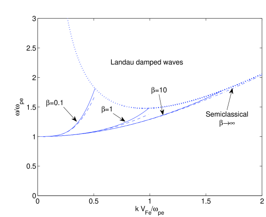
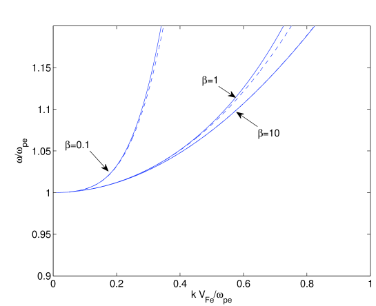
In Figs. 1 and 2, we show dispersion curves for the high-frequency ($\omega\gg\omega_{pi}$) waves for different values of $\beta$, obtained from the solutions of the dispersion relation (10), by using the electron susceptibility (21), as well as the expansion (23) and the limiting semi-classical case (22). We have also indicated the border between undamped and Landau damped waves, obtained from (24) and (25). We note that the dispersion curve for the semiclassical case in Fig 1 always lies in the undamped regime, below the border between undamped and Landau damped waves. For the undamped waves, the expansion (23) approximates the exact dispersion relation within a few percent, and can therefore be used instead of (21) for most cases. This holds especially for small wavenumbers, as can be seen in the closeup in Fig. 2.

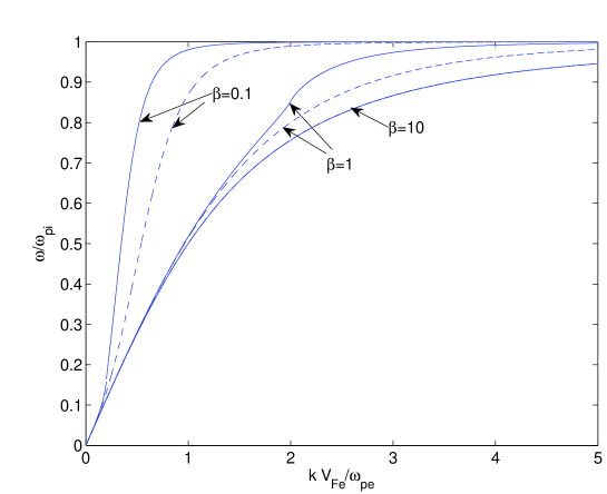
The dispersion curves for the low-frequency ion-acoustic oscillations are plotted in Fig. 3, were we have depicted the $\omega$ in (29) for $\chi_{e}$ given by the exact expression (26) and the approximate expansion (27), and for different values of $\beta$. We note that the dispersion curves show agreement at small wavenumbers but deviate significantly for larger wavenumbers in the case $\beta=0.1$, while the agreement is better for $\beta=1$ and excellent for $\beta=10$. It should be kept in mind that when $\hbar k\sim m_{e}V_{Fe}$ then the wavelength of the oscillations is comparable to the inter-particle distance, and there will be corrections due to the discrete nature of the ion background. Thus, the theory is not valid for oscillations with $\hbar k\gg m_{e}V_{Fe}$.

VII Conclusions

In this paper, we have here studied the dispersion properties of electrostatic oscillations in quantum plasmas for different parameters ranging from semiconductor plasmas, to typical metallic electron densities and to densities corresponding to compressed matter and dense astrophysical objects. We have derived a simplified expansion that accurately approximates the exact dispersion relation for small wavenumbers. The possibility of Landau damping due to quantum tunneling effects at large wavenumbers has also been discussed, and conditions for Landau damping has been derived. The present results should be useful in understanding the salient features of electrostatic plasma oscillations in dense plasmas with degenerate electrons. The latter are encountered in metals, in highly compressed intense laser-solid density plasma experiments, and in compact astrophysical objects (e.g. interior of white dwarf stars).

Acknowledgements.
This work was supported by the Deutsche Forschungsgemeinschaft through the project SH21/3-1 of the Research Unit 1048, and by the Swedish Research Council (VR).

References

  • Azechiet al. (1991) Azechi H. et al. 1991 High-Density Compression Experiments at ILE, Osaka. Laser Part. Beams 9, 193–207.
  • Azechi et al. (2006) Azechi H. et al. 2006 Present Status of the FIREX Programme for the Demonstration of Ignition and Burn. Plasma Phys. Control. Fusion 48, B267–B275.
  • Bohm (1952) Bohm D. 1952. A Suggested Interpretation of the Quantum Theory in Terms of ”Hidden” Variables. I. Phys. Rev. 85, 166–179.
  • Bohm and Pines (1953) Bohm, D. and Pines, D. 1953 A Collective Description of Electron Interactions: III. Coulomb Interactions in a Degenerate Gas. Phys. Rev. 92, 609–625.
  • Bonitz et al. (2003) Bonitz M., Semkat D., Filinov A. et al. 2003 Theory and Simulation of Strong Correlations in Quantum Coulomb Systems. J. Phys. A: Math. Gen. 36, 5921–5930.
  • Chandrasekhar (1935) Chandrasekhar S. 1935 The Highly Collapsed Configurations of a Stellar Mass (second paper). MNRAS 95, 207–225.
  • Crouseilles (2008) Crouseilles N., Hervieux, P. A., and Manfredi G. 2008 Quantum Hydrodynamic Models for Nonlinear Electron Dynamics in Thin Metal Films. Phys. Rev. B 78 155412.
  • Ferrel (1957) Ferrel R. A. 1957 Characteristic Energy Loss of Electrons Passing through Metal Foils. II. Dispersion Relation and Short Wavelength Cutoff for Plasma Oscillations Phys. Rev. 107, 450–462.
  • Glenzer et al. (2007) Glenzer S. H., Landen, O. L., Neumayer, P., et al. 2007 Observations of Plasmons in Warm Dense Matter, Phys. Rev. Lett. 98 065002.
  • Klimontovich and Silin (1952) Klimontovich Y. L. and Silin V. P. 1952 Doklady Akad. Nauk S. S. S. R. 82 361.; 1952 JFTF (Journal Experimental Teoreticheskoi Fisiki) 23 151.
  • Klimontovich and Silin (1961) Klimontovich Y. and Silin V. P. 1961 The Spectra of Systems of Interacting Particles. In Plasma Physics, Ed. J. E. Drummond (McGraw-Hill, New York) Chap. 2 pp. 35–87.
  • Kritcher et al. (2008) Kritcher A. L. et al. 2008 Ultrafast X-ray Thomson Scattering of Shock-Compressed Matter. Science 322 69–71.
  • Lee et al. (2009) Lee H. J. et al. 2009 X-Ray Thomson-Scattering Measurements of Density and Temperature in Shock-Compressed Beryllium. Phys. Rev. Lett. 102 115001.
  • Lindl (1995) Lindl J. 1995 Development of the Indirect-Drive Approach to Inertial Confinement Fusion and the Target Physics Basis for Ignition and Gain. Phys. Plasmas 2, 3933.
  • Manfredi (2005) Manfredi G. 2005 How to Model Quantum Plasmas. Fields Inst. Commun. 46 263–287.
  • Mendonça et al. (2008) Mendonça, J. T., Ribeiro, E. and Shukla, P. K. 2008 Wave kinetic description of quantum electron-positron plasmas. J. Plasma Phys., 74, 91–94.
  • Pines (1961) Pines D. 1961 I. Quantum Plasma Physics: Classical and Quantum Plasmas. J. Nucl. Energy: Part C: Plasma Phys. 2 5–17.
  • Serbeto (2008) Serbeto A., Mendonça J. T., Tsui K. H. & Bonifacio R. 2008 Quantum Wave Kinetics of High-Gain Free-Electron Lasers. Phys. Plasmas 15, 013110.
  • Shaikh and Shukla (2007) Shaikh D. and Shukla P. K. 2007 Fluid Turbulence in Quantum Plasmas. Phys. Rev. Lett. 99, 125002.
  • Shukla and Eliasson (2006) Shukla P. K. and Eliasson B. 2006 Formation and Dynamics of Dark Solitons and Vortices in Quantum Electron Plasmas. Phys. Rev. Lett. 96, 245001.
  • Shukla (2009) Shukla P. K. 2009 A New Spin on Quantum Plasmas. Nature Phys. 5, 92–93.
  • Son and Fisch (2005) Son S. and Fisch N. J. 2005 Current-Drive Efficiency in a Degenerate Plasma Phys. Rev. Lett. 95 225002.
  • Tabak et al. (1994) Tabak M. et al. 1994 Ignition and High Gain with Ultrapowerful Lasers Phys. Plasmas 1, 1626–1634.
  • Tabak et al. (2005) Tabak M. et al. 2005 Review of Progress in Fast Ignition Phys. Plasmas 12 057305.
  • Watanabe (1956) Watanabe H. 1956 Experimental Evidence for the Collective Nature of the Characteristic Energy Loss of Electrons in Solids –Studies on the Dispersion Relation of Plasma Frequency– J. Phys. Soc. Jpn 11, 112–119.