Sampling the Fermi statistics
and other conditional product measures

Abstract

Through a Metropolis-like algorithm with single step computational cost of order one, we build a Markov chain that relaxes to the canonical Fermi statistics for $k$ non-interacting particles among $m$ energy levels. Uniformly over the temperature as well as the energy values and degeneracies of the energy levels we give an explicit upper bound with leading term $km\ln k$ for the mixing time of the dynamics. We obtain such construction and upper bound as a special case of a general result on (non-homogeneous) products of ultra log-concave measures (like binomial or Poisson laws) with a global constraint. As a consequence of this general result we also obtain a disorder-independent upper bound on the mixing time of a simple exclusion process on the complete graph with site disorder. This general result is based on an elementary coupling argument, illustrated in a simulation appendix and extended to (non-homogeneous) products of log-concave measures.

Key words: Metropolis algorithm, Markov chain, sampling, mixing time, product measure, conservative dynamics.

AMS 2010 classification: 60J10, 82C44.

1 From the Fermi statistics to general conditional products of log-concave measures

1.1 Sampling the Fermi statistics

Given two positive integers $k$ and $m$, given a non-negative real number $\beta$, given $m$ real numbers $v_{1}$, …, $v_{m}$ and given $m$ integers $n_{1}$, …, $n_{m}$ such that

$$n:=\sum_{j=1}^{m}n_{j}\geq k,$$ (1.1)

the canonical Fermi statistics at inverse temperature $\beta$ for $k$ non-interacting particles among the $m$ energy levels $1$, …, $m$, with energy values $v_{1}$, …, $v_{m}$ and degeneracies $n_{1}$, …, $n_{m}$ is the conditional probability measure on

$${\cal X}_{k,m}:=\left\{(k_{1},\dots,k_{m})\in{\mathbb{N}}^{m}:\>k_{1}+\cdots+k_{m}=k\right\}$$ (1.2)

given by

$$\nu:=\mu(\cdot|{\cal X}_{k,m})$$ (1.3)

with $\mu$ the product measure on ${\mathbb{N}}^{m}$ such that

$$\mu(k_{1},\dots,k_{m}):=\frac{1}{Z}\prod_{j=1}^{m}\binom{n_{j}}{k_{j}}\exp\{-\beta k_{j}v_{j}\},$$ (1.4)

$$Z:=\sum_{k_{1},\dots,k_{m}}\prod_{j=1}^{m}\binom{n_{j}}{k_{j}}\exp\{-\beta k_{j}v_{j}\},$$ (1.5)

with $\binom{n_{j}}{k_{j}}=0$ whenever $k_{j}>n_{j}$. In other words, $\nu$ is a (non-homogeneous) product of binomial laws in $k_{1}$, …, $k_{m}$ with the global constraint

$$k_{1}+\dots+k_{m}=k$$ (1.6)

and we can write

$$\nu(k_{1},\dots,k_{m})=\frac{1}{Q}\prod_{j=1}^{m}e^{\phi_{j}(k_{j})},\quad(k_{1},\dots,k_{m})\in{\cal X}_{k,m}$$ (1.7)

where the $\phi_{j}$ are defined by

$$\phi_{j}:k_{j}\in{\mathbb{N}}\mapsto-\beta k_{j}v_{j}+\ln\binom{n_{j}}{k_{j}}\in{\mathbb{R}}\cup\{-\infty\}$$ (1.8)

and $Q$ is such that $\nu$ is a probability measure.

The first aim of this paper is to describe an algorithm that simulates a sampling according to $\nu$ in a time that can be bounded from above by an explicit polynomial in $k$ and $m$, uniformly over $\beta$, $(v_{j})_{1\leq j\leq m}$ and $(n_{j})_{1\leq j\leq m}$. The reason why we prefer a bound in $k$ and $m$ rather than in the ‘volume’ of the system $n=\sum_{j}n_{j}$, will be clarified later.

A first naive (and wrong) idea to do so consists in choosing the position (the energy level) of a first, second, … and eventually $k^{\rm th}$ particle in the following way. First choose randomly the position of the first particle according to the exponential weights associated with the ‘free entropies’ of the empty sites, that is choose level $j$ with a probability proportional to $\exp\{-\beta v_{j}+\ln n_{j}\}$. Then decrease by 1 the degeneracy of the chosen energy level and repeat the procedure to choose the position of the second, third, … and eventually $k^{\rm th}$ particle. It is easy to check that, doing so, the final distribution of the occupation numbers $k_{1}$, …, $k_{m}$ associated with the different energy levels, that is of the numbers of particles placed in each level, is in general not given by $\nu$ as soon as $k$ is larger than one. But it turns out that this naive idea can be adapted to build an efficient algorithm to perform approximate samplings under the Fermi statistics.

Very classically, the fast sampling performed by the algorithm we will build will be obtained by running a Markov chain $X$ with transition matrix $p$ on ${\cal X}_{k,m}$ and with equilibrium measure $\nu$. The efficiency of the algorithm will be measured through the bounds that we will be able to give on the mixing time $t_{\epsilon}$, defined for any positive $\epsilon<1$ by

$$t_{\epsilon} := \inf\{t\geq 0:\>d(t)\leq\epsilon\}$$ (1.9)

$$d(t) := \max_{\eta\in{\cal X}_{k,m}}\|p^{t}(\eta,\cdot)-\nu\|_{\rm TV}$$ (1.10)

where $\|\cdot\|_{\rm TV}$ stands for the total variation distance defined for any probability measures $\nu_{1}$ and $\nu_{2}$ on ${\cal X}_{k,m}$ by

$$\|\nu_{1}-\nu_{2}\|_{\rm TV}:=\max_{A\subset{\cal X}_{k,m}}|\nu_{1}(A)-\nu_{2}(A)|=\frac{1}{2}\sum_{\eta\in{\cal X}_{k,m}}|\nu_{1}(\eta)-\nu_{2}(\eta)|.$$ (1.11)

As a consequence, estimating mixing times is not the only one issue of this paper, building a ‘good’ Markov chain is part of the problem.

As far as that part of the problem is concerned, we propose to build a Metropolis-like algorithm that uses the ‘free energies’ of the naive approach to define a conservative dynamics. Assuming that at time $t\in{\mathbb{N}}$ the system is in some configuration $X_{t}=\eta$ in ${\cal X}_{k,m}$ with $\nu(\eta)>0$, and defining for any $\eta=(k_{1},\dots,k_{m})$ and any distinct $i$ and $j$ in $\{1;\cdots;m\}$

$$\eta^{ij}:=(k^{\prime}_{1},\dots,k^{\prime}_{m})\quad\mbox{with}\quad k^{\prime}_{s}=\left\{\begin{array}[]{ll}k_{s}&\mbox{for $s\in\{1;\cdots;m\}\setminus\{i;j\}$}\\ k_{i}-1&\mbox{if $s=i$}\\ k_{j}+1&\mbox{if $s=j$}\end{array}\right.,$$ (1.12)

the configuration at time $t+1$ will be decided as follows:

• choose a particle with uniform probability (it will stand in a given level $i$ with probability $k_{i}/k$),

• choose an energy level with uniform probability (a given level $j$ will be chosen with probability $1/m$),

• with $i$ the level where stood the chosen particle and $j$ the chosen energy level, extract a uniform variable $U$ on $[0;1)$ and set $X_{t+1}=\eta^{ij}$ if $i\neq j$ and

  $$U<\exp\{-\beta v_{j}+\ln(n_{j}-k_{j})+\beta v_{i}-\ln(n_{i}-(k_{i}-1))\},$$ (1.13)

  $X_{t+1}=\eta$ if not.

In other words, denoting by $[a]^{+}=(a+|a|)/2$ the positive part of any real number $a$ and with

$$\psi_{j}:k_{j}\in\{0;\cdots;n_{j}\}\mapsto-\beta v_{j}+\ln(n_{j}-k_{j})\in{\mathbb{R}}\cup\{-\infty\},\quad j\in\{1;\cdots;m\},$$ (1.14)

for any distinct $i$ and $j$ in $\{1;\cdots;m\}$

$$P(X_{t+1}=\eta^{ij}|X_{t}=\eta)=p(\eta,\eta^{ij})=\frac{k_{i}}{k}\frac{1}{m}\exp\{-[\psi_{i}(k_{i}-1)-\psi_{j}(k_{j})]^{+}\},$$ (1.15)

and

$$P(X_{t+1}=\eta|X_{t}=\eta)=p(\eta,\eta)=1-\sum_{i\neq j}p(\eta,\eta^{ij}).$$ (1.16)

Remark: In order to avoid any ambiguity in (1.15) in the case $k_{i}=0$, we set $\psi_{i}(-1)=+\infty$ (even though the algorithm we described does not require any convention for $\psi_{i}(-1)$).

This Markov chain is certainly irreducible and aperiodic. To prove that it relaxes to $\nu$ we will check the reversibility of the process with respect to $\nu$. Then we will have to estimate the mixing time of the process. We will carry out both the tasks in a more general setup.

1.2 A general result

For any function $f:{\mathbb{N}}\rightarrow{\mathbb{R}}$ we define

$$\nabla^{+}f:x\in{\mathbb{N}}\mapsto\nabla^{+}_{x}f:=f(x+1)-f(x)$$ (1.17)

$$\nabla^{-}f:x\in{\mathbb{N}}\setminus\{0\}\mapsto\nabla^{-}_{x}f:=f(x-1)-f(x)$$ (1.18)

$$\Delta f:x\in{\mathbb{N}}\setminus\{0\}\mapsto\Delta_{x}f:=\nabla_{x}^{+}f+\nabla_{x}^{-}f=-\nabla^{-}_{x}(\nabla^{+}f)$$ (1.19)

and we say that a measure $\gamma$ on the integers

$$\gamma:x\in{\mathbb{N}}\mapsto e^{\phi(x)}\in{\mathbb{R}}_{+},$$ (1.20)

with $\phi:{\mathbb{N}}\rightarrow{\mathbb{R}}\cup\{-\infty\}$, is log-concave if ${\mathbb{N}}\setminus\gamma^{-1}(\{0\})$ is an interval of the integers and

$$\gamma(x)^{2}\geq\gamma(x-1)\gamma(x+1),\quad x\in{\mathbb{N}}\setminus\{0\},$$ (1.21)

i.e., if $\nabla^{+}\phi$ is non-increasing, or, equivalently, $-\Delta\phi$ is non-negative (with the obvious extension of the previous definitions to such a possibly non-finite $\phi$). The measure $\mu$ defined in (1.4) is a product of log-concave measures and the canonical Fermi statistics is such a product measure normalized over the condition (1.6).

N.B. From now on, and except for explicit mentioning of additional hypotheses, we will only assume that the probability measure $\nu$ we want to sample is a product of log-concave measures normalized over the global constraint (1.6), i.e., that $\nu$ is a probability on ${\cal X}_{k,m}$ that can be written in the form (1.7) with non-increasing $\nabla^{+}\phi_{j}$’s.

In this more general setup we will often refer to the indices $j$ in $\{1;\cdots;m\}$ as sites rather than energy levels of the system.

Actually the $e^{\phi_{j}}$’s of the Fermi statistics are much more than log-concave measures. They are ultra log-concave measures according to the following definition by Pemantle [2] and Liggett [3].

Definition 1.2.1

A measure $\gamma:{\mathbb{N}}\rightarrow{\mathbb{R}}_{+}$ is ultra log-concave if $x\mapsto x!\gamma(x)$ is log-concave.

In other words $e^{\phi_{j}}$ is ultra log-concave if and only if

$$\psi_{j}:=\nabla^{+}\phi_{j}+\ln(1+\cdot)$$ (1.22)

is non-increasing (for the Fermi statistics observe that so are the $\phi_{j}$’s and that (1.22) is consistent with (1.14)).

For birth and death processes that are reversible with respect to ultra log-concave measures, Caputo, Dai Pra and Posta [10] proved modified log-Sobolev inequalities and stronger convex entropy decays, both giving good upper bounds on the mixing time of the processes. Johnson [13] proved also easier Poincaré inequalities that give weaker bounds on the mixing times. We refer to [4], [5], [9] for an introduction to this classical functional inequality approach to convergence to equilibrium and we note that for such birth and death processes the ultra-log concavity hypotheses allowed for a Bakry-Émery like approach (see [1]) to derive (modified) log-Sobolev inequalities. Actually, [10] was an attempt to extend this celebrated analysis to Markov processes with jumps (see also [15] for a more geometric perspective). But it turns out, as we will soon review, that beyond the case of birth and death processes the role of ultra log-concavity to follow the Bakry-Émery line in the discrete setup is still unclear.

In this paper we will not follow the functional analysis approach to control mixing times. To bound from above the mixing time of a Markov chain that is reversible with respect to a conditional product of ultra log-concave measures, we will follow (and recall in Section 2) the non less classical, and, in this case, elementary, probabilistic approach via coalescent coupling. We will prove:

Theorem 1

If $\nu$ derives from a product of ultra log-concave measures, then the Markov chain with transition matrix $p$ defined by

$$p(\eta,\eta^{ij}) = \frac{k_{i}}{k}\frac{1}{m}\exp\{-[\psi_{i}(k_{i}-1)-\psi_{j}(k_{j})]^{+}\},$$ (1.23)

$$\qquad\eta=(k_{1},\dots,k_{m})\in{\cal X}_{k,m}\setminus\nu^{-1}\{0\},$$

$$\qquad i\neq j\in\{1;\cdots;m\},$$

$$p(\eta,\eta) = 1-\sum_{i\neq j}p(\eta,\eta^{ij})$$ (1.24)

is reversible with respect to $\nu$ and, for any positive $\epsilon<1$, its mixing time $t_{\epsilon}$ satisfies

$$t_{\epsilon}\leq km\ln(k/\epsilon).$$ (1.25)

Proof: see Section 2.

The most relevant point of Theorem 1 with respect to the previous results we know stands in the uniformity of the upper bound above the disorder of the system (except for the ultra log-concavity hypothesis on $e^{\phi_{j}}$ in each $j$). In particular and as far as the Fermi statistics is concerned, our estimate does not depend on the temperature, and, more generally it is independent from the energy values as well as the level degeneracies.

To illustrate this fact let us start with the case $n_{j}=1$ for all $j$. In this case our dynamics is a simple exclusion process with site disorder. Caputo ([6], [12]) proved Poincaré inequalities for such processes, in their continuous time version, assuming a uniform lower (and upper) bound on general transition rates, while Caputo, Dai Pra and Posta [10], looking at particular rates for the process and still assuming moderate disorder – that is, uniform lower and upper bounds on these rates – proved a modified log-Sobolev inequality. For the particular choice of rates they made, the upper bound on the mixing time implied by [10] could not hold in a strong disorder context (for example with $k=1$, $m=3$, $v_{1}=v_{2}=0$, $v_{3}>0$ and $\beta\gg 1$). Our uniformity over the disorder of the system depends then strongly on our particular choice for the transition probabilities. As it is often the case with Markov processes on discrete state space, the details of the dynamics are not less important than the properties of its equilibrium measure.

Under the moderate disorder hypotheses of [6], [10], [12], however, the upper bound on the mixing time implied by [10] and suggested by [6], [12] is better than our upper bound in Theorem 1 (by a factor of order $k$). But we will see that introducing such moderate disorder hypotheses in our arguments directly improves our result by a factor of order $m\geq k$ (see the last remark at the end of Section 2).

To close the discussion on simple exclusion processes we note that those of the arguments in [12] that do not depend on the disorder suggest an upper bound on the mixing time of order $m^{2}\ln m$. Theorem 1 improves this estimate when $k$ is small with respect to $m$.

As far as more general conditional non-homogeneous product of log-concave measures are concerned, we stress once again that Theorem 1 gives a uniform bound over the disorder that can be improved by a factor of order $m$ by adding moderate disorder hypotheses (see the last remark at the end of Section 1.4 and our simulation Appendix). Then, such product measures can be equilibrium measures of zero-range processes with a continuous time generator as in [8], [10]:

$${\cal L}_{\eta}f:=\frac{1}{m}\sum_{i\neq j}c_{i}(k_{i})\Big{(}f(\eta^{ij})-f(\eta)\Big{)}.$$ (1.26)

where the $c_{j}:k_{j}\in{\mathbb{N}}\mapsto[0,+\infty)$ are such that $c_{j}(0)=0$ and $c_{j}(k_{j})>0$ for $k_{j}>0$. Indeed, such a process is reversible with respect to $\nu$ provided that

$$\forall j\in\{1;\cdots;m\},\;\forall k_{j}\in{\mathbb{N}},\;\phi_{j}(k_{j})=\sum_{0<l\leq k_{j}}\ln\frac{1}{c_{j}(l)}\;.$$ (1.27)

Boudou, Caputo, Dai Pra and Posta [8] proved a Poincaré inequality for such a process, assuming that there exists a positive $c$ such that

$$\forall j\in\{1;\cdots;m\},\;\forall k_{j}\in{\mathbb{N}},\;c_{j}(k_{j}+1)-c_{j}(k_{j})\geq c.$$ (1.28)

This is a moderate disorder hypothesis that implies the log-concavity of the $\mu_{j}$. To go to modified log-Sobolev inequalities, i.e., to good mixing time estimates rather than simple gap estimates, there is the additional hypothesis in [10] that there exists a non-negative $\delta<c$ such that

$$\forall j\in\{1;\cdots;m\},\;\forall k_{j}\in{\mathbb{N}},\;c_{j}(k_{j}+1)-c_{j}(k_{j})\leq c+\delta.$$ (1.29)

Clearly there are ultra log-concave measures that do not satisfy (1.29): to have an ultra log-concave measure one needs a strongly decreasing $\nabla^{+}\phi_{j}$, i.e., a strongly increasing $c_{j}$. Conversely, it is not true that (1.28) and (1.29) imply ultra log-concavity, i.e.,

$$\forall j\in\{1;\cdots;m\},\;\forall k_{j}\geq 1,\;\ln\frac{k_{j}+1}{c_{j}(k_{j}+1)}\leq\ln\frac{k_{j}}{c_{j}(k_{j})}\;.$$ (1.30)

However, elementary algebra shows that (1.28) together with (1.29) implies

$$\forall j\in\{1;\cdots;m\},\;\forall k_{j}\geq 1,\;\ln\frac{k_{j}+1/2}{c_{j}(k_{j}+1)}\leq\ln\frac{k_{j}}{c_{j}(k_{j})}$$ (1.31)

and this strangely looks like (1.30). Therefore we said that the role played by ultra log-concavity is still unclear along the functional analysis line of research in the discrete setup. We conclude stressing once again that in this paper we will follow a different line, that our uniform bound on the mixing time comes from an elementary coupling argument and that we do not need any moderate disorder hypothesis.

1.3 Interpolating between sites and particles

It seems that today available techniques are such that the less log-concavity we have, the more homogeneity we need to control the convergence to equilibrium. Staying to the papers mentioned above, without ultra log-concavity or at least something that looks like ultra log-concavity we only have Poincaré inequalities for non-homogeneous product of log-concave measures, and without log-concavity we have modified log-Sobolev inequalities for homogeneous product measures only (see [10]). In addition, the only result we know for a conservative dynamics in (weakly) disordered context and with an equilibrium measure that is a product of measures that are not log-concave is that of Landim and Noronha Neto [7] for the (continuous) Ginzburg-Landau process.

We will see that all the ideas of the proof of Theorem 1 can be extended to deal with a large class of conditional product of log-concave measures that are not ultra log-concave. To do so, let us define

$$\delta:=\max\left\{\lambda\in[0;1]:\>\forall j\in\{1;\cdots;m\},\,\forall k_{j}>0,\,-\Delta_{k_{j}}\phi_{j}\geq\lambda\ln\frac{1+k_{j}}{k_{j}}\right\}.$$ (1.32)

In other words, $\delta$ is the largest real number in $[0;1]$ for which all the

$$\psi_{j}^{[\delta]}:=\nabla^{+}\phi_{j}+\delta\ln(1+\cdot),\quad j\in\{1;\cdots;m\},$$ (1.33)

are non-increasing. Denoting by $a\wedge b$ the minimum of two real numbers $a$, $b$ and defining

$$l_{\delta}:=k^{\delta}(k\wedge m)^{1-\delta}$$ (1.34)

we will prove:

Theorem 2

If $\delta>0$ then the Markov chain with transition matrix $p$ defined by

$$p(\eta,\eta^{ij}) = \frac{k_{i}^{\delta}}{l_{\delta}}\frac{1}{m}\exp\left\{-\left[\psi_{i}^{[\delta]}(k_{i}-1)-\psi_{j}^{[\delta]}(k_{j})\right]^{+}\right\},$$ (1.35)

$$\qquad\eta=(k_{1},\dots,k_{m})\in{\cal X}_{k,m}\setminus\nu^{-1}\{0\},$$

$$\qquad i\neq j\in\{1;\cdots;m\},$$

$$p(\eta,\eta) = 1-\sum_{i\neq j}p(\eta,\eta^{ij})$$ (1.36)

is reversible with respect to $\nu$ and, for any positive $\epsilon<1$, its mixing time $t_{\epsilon}$ satisfies

$$t_{\epsilon}\leq\frac{(k\wedge m)^{1-\delta}}{\delta}km\ln(k/\epsilon).$$ (1.37)

Remark 1: By Hölder’s inequality, if $\delta>0$ then

$$\sum_{i=1}^{m}k_{i}^{\delta}=\sum_{i=1}^{m}k_{i}^{\delta}{\tt 1\tt l}^{1-\delta}_{\{k_{i}\neq 0\}}\leq\bigg{(}\sum_{i=1}^{m}k_{i}\bigg{)}^{\delta}\bigg{(}\sum_{i=1}^{m}{\tt 1\tt l}_{\{k_{i}\neq 0\}}\bigg{)}^{1-\delta}\leq l_{\delta}$$ (1.38)

and this ensures that (1.35)-(1.36) define a probability matrix.

Remark 2: As far as this can make sense in our discrete setup, we note that the hypothesis $\delta>0$ is slightly weaker than a “uniform strict log-concavity hypothesis” (see (1.32)).

Proof of Theorem 2: see Section 3.

For $\delta=1$ the transition matrix represents an algorithm starting with a uniform choice of a particle. For $\delta=0$ Theorem 2 is empty but (1.35)-(1.36) still define a Markov chain $X$ that can be seen as a particular version of a discrete state space non-homogeneous Ginzburg-Landau process. In this case the transition matrix represents an algorithm that starts with a uniform choice of a (non-empty) site. The case $0<\delta<1$ can be seen as an interpolation between uniform choices of site and particle. More precisely, assuming that at time $t\in{\mathbb{N}}$ the system is in some configuration $X_{t}=\eta=(k_{1},\dots,k_{m})$ in ${\cal X}_{k,m}\setminus\nu^{-1}\{0\}$, the configuration at time $t+1$ can be decided as follows.

• Choose a site $i$ or no site at all with probabilities proportional to $k_{i}^{\delta}$ and $l_{\delta}-\sum_{i}k_{i}^{\delta}$.

• If some site $i$ was chosen, then proceed as in the previously described algorithm using the functions $\psi_{j}^{[\delta]}$ instead of the $\psi_{j}$’s, if not, then set $X_{t+1}=\eta$.

1.4 Last remarks and original motivation

First, we note that as long as one wants bounds that are uniform over the disorder, Theorem 1 gives the right order for the mixing time: for the Fermi statistic in the very low temperature regime with, for example, $v_{1}<v_{2}<\dots<v_{m}$ and $n_{1},n_{2}\geq k$, the equilibrium measure will be concentrated on $(k,0,\dots,0)$ while, starting from $(0,k,0,\dots,0)$, the system will reach the ground state in a time of order $km\ln k$ for large $k$ (this is a coupon-collector estimate). This fact is illustrated in our simulation Appendix.

Next, we observe that, with our definitions, $p(\eta,\eta)$ can often be close to one, especially in strong disorder situations or when the right and left hand sides in (1.38) are far from each other. If one would like to use these results to perform practical simulations, then it could be useful to note that the computational time would still be improved by implementing an algorithm that at each step simulates, for a given configuration $\eta$ on the trajectory of the Markov chain, the elapsed time before the particle reach a different configuration (this is a geometric time) and choose this configuration $\eta^{\prime}\neq\eta$ according to the (easy to compute) associated law. It would then be enough to stop the algorithm as soon as the total simulated time goes beyond the mixing time (and then return the last configuration, that the system occupied at the mixing time) rather than waiting for the original algorithm to make a step number equal to the mixing time.

Turning back to the first naive and wrong idea, it is interesting to note that it can easily be modified to determine the most probable states of the system, i.e., the configurations $\eta^{*}=(k_{1}^{*},\dots,k_{m}^{*})$ in ${\cal X}_{k,m}$ such that

$$\sum_{j=1}^{m}\phi_{j}(k_{j}^{*})=\max_{k_{1}+\cdots+k_{m}=k}\sum_{j=1}^{m}\phi_{j}(k_{j}).$$ (1.39)

One can prove, using the concavity of the $\phi_{j}$’s, that the most probable configurations for the system with $k$ particles can be obtained from the most probable configurations $(k^{\prime}_{1},\dots,k^{\prime}_{m})$ for the system with $k-1$ particles simply adding one particle where the corresponding gain in ‘free energy’ is the highest, that is in $j^{*}$ such that

$$\nabla^{+}_{k^{\prime}_{j^{*}}}\phi_{j^{*}}=\max_{j}\nabla^{+}_{k^{\prime}_{j}}\phi_{j}.$$ (1.40)

As a consequence one can place the particles one by one, each time maximizing this free energy gain, to build the most probable configuration.

Then, as a referee pointed out, since the sampling problem is a trivial one in the Poissonian case (when all the $\mu_{j}$’s are Poisson measures, so that $\nu$ is nothing but a multinomial law $M$), one can ask about the expected time needed to perform a rejection sampling with respect to the multinomial case. It is given by $\max_{\eta}\nu(\eta)/M(\eta)$. If we take the Fermi statistics with $m=k$ and all the $n_{j}$ equal to 1, then we find (optimizing on the multinomial parameters by a geometric/arithmetic mean comparison) $k^{k}/k!\sim e^{k}/\sqrt{2\pi k}$. Of course, the sampling problem for that Fermi statistics is also a trivial one. But if we take $\beta=0$ and all the $n_{j}$ equal to 2, it is not anymore a trivial problem and we find an expected time for the rejection sampling that is logarithmically equivalent to $(e/2)^{k}$.

Turning back to the Fermi statistics we now explain why we were interested in bounds in $k$ and $m$ rather than in the volume $n$. Iovanella, Scoppola and Scoppola defined in [11] an algorithm to individuate cliques (i.e., complete subgraphs) with $k$ vertices inside a large Erdös-Reyni random graph with $n$ vertices. Their algorithm requires to perform repeated approximate samplings of Fermi statistics in volume $n$, with $k$ particles and $m=2k+1$ energy levels. Now, the key observation is that the largest cliques in Erdös-Reyni graphs with $n$ vertices are of order $\ln n$, so that $k$ and $m$ in this problem are logarithmically small with respect to $n$. Before Theorem 1 the samplings for their algorithm were done by running simple exclusion processes with $k$ particles on the complete graph (with site disorder) of size $n$. Such processes converge to equilibrium in a time of order $kn\ln k$. Now the samplings are done in a time of order $km\ln k\sim 2k^{2}\ln k$, and that was the original motivation of the present work.

Finally we note that our bound in $k$ and $m$ is not only useful when $k$ is small with respect to $n$ but also when $k$ is close to $n$. In this case we can define a dynamics on the $n-k$ vacancies rather than on the $k$ particles.

2 Proof of Theorem 1

In this section we assume that $\nu$ is a measure on ${\cal X}_{k,m}$ deriving from a product of ultra log-concave measures, which means that we can write $\nu(k_{1},\ldots,k_{m})=(1/Q)\prod_{j}e^{\phi_{j}(k_{j})}$ and, for all $j\in\{1;\cdots;m\}$, $\psi_{j}$ defined by (1.22) is non-increasing.

2.1 Reversibility

We first prove that the transition matrix $p$ defined by (1.23) and (1.24) is reversible with respect to the measure $\nu$. Let $\eta=(k_{1},\ldots,k_{m})\in{\cal X}_{k,m}\setminus\nu^{-1}\{0\}$ and let $i\not=j\in\{1;\cdots;m\}$. We have $p(\eta,\eta^{ij})\neq 0$ if and only if $\nu(\eta^{ij})\neq 0$ and, in that case,

$$\frac{\nu(\eta^{ij})}{\nu(\eta)}=\frac{e^{\phi_{i}(k_{i}-1)+\phi_{j}(k_{j}+1)}}{e^{\phi_{i}(k_{i})+\phi_{j}(k_{j})}}=\exp\{\nabla_{k_{i}}^{-}\phi_{i}+\nabla^{+}_{k_{j}}\phi_{j}\}$$ (2.1)

while

$$\frac{p(\eta^{ij},\eta)}{p(\eta,\eta^{ij})} = \frac{k_{j}+1}{k_{i}}\exp\{-[\psi_{j}(k_{j})-\psi_{i}(k_{i}-1)]^{+}$$ (2.2)

$$\qquad\qquad\qquad+[\psi_{i}(k_{i}-1)-\psi_{j}(k_{j})]^{+}\}$$

$$= \exp\{\psi_{i}(k_{i}-1)-\psi_{j}(k_{j})+\ln(k_{j}+1)-\ln(k_{i})\}$$ (2.3)

$$= \exp\{\nabla^{+}_{k_{i}-1}\phi_{i}-\nabla^{+}_{k_{j}}\phi_{j}\}$$ (2.4)

$$= \exp\{-\nabla_{k_{i}}^{-}\phi_{i}-\nabla^{+}_{k_{j}}\phi_{j}\}$$ (2.5)

so that

$$\nu(\eta)p(\eta,\eta^{ij})=\nu(\eta^{ij})p(\eta^{ij},\eta).$$ (2.6)

2.2 A few words about the coupling method

In order to upper bound the mixing time of the Markov chain with transition matrix $p$, we will use the coupling method. Given a Markov chain $(X^{1},X^{2})$ on ${\cal X}_{k,m}\times{\cal X}_{k,m}$, we say it is a (Markovian) coupling for the dynamics if both $X^{1}$ and $X^{2}$ are Markov chains with transition matrix $p$. Given such a coupling, we define the coupling time $\tau_{\rm couple}$ as the first (random) time for which the chains meet, that is

$$\tau_{\rm couple}:=\inf\{t\geq 0:X^{1}_{t}=X^{2}_{t}\}.$$ (2.7)

In this work, every coupling will also satisfy the condition

$$t\geq\tau_{\rm couple}\Rightarrow X^{1}_{t}=X^{2}_{t}.$$ (2.8)

Then, it is a well-known fact that for all $t\geq 0$,

$$d(t)\leq\max_{\eta,\theta\in{\cal X}_{k,m}}P(\tau_{\rm couple}>t|X^{1}_{0}=\eta,X^{2}_{0}=\theta)$$ (2.9)

where $d(t)$ is defined by (1.10). A proof of this fact as well as an exhaustive introduction to mixing time theory can be found in [14].

In the proof of both 1 and 2 we will build a coupling for which there exists a function $\rho$ that measures in some sense a ‘distance’ between $X^{1}_{t}$ and $X^{2}_{t}$ and from which we will get a bound on the mixing time thanks to the following proposition.

Proposition 2.2.1

Let $(X^{1},X^{2})$ be a coupling for a Markov chain with transition matrix $p$. We assume that the coupling satisfies the property (2.8). Let $\rho:{\cal X}_{k,m}\times{\cal X}_{k,m}\rightarrow{\mathbb{N}}$ such that $\rho(\eta,\theta)=0$ if and only if $\eta=\theta$. If $M$ is the maximum of $\rho$ and if there exists $\alpha>1$ such that, for all $t\geq 0$,

$$E\left(\rho(X^{1}_{t+1},X^{2}_{t+1})|X^{1}_{t},X^{2}_{t}\right)\leq\left(1-\frac{1}{\alpha}\right)\rho(X^{1}_{t},X^{2}_{t}),$$ (2.10)

then for all $\epsilon>0$ the mixing time $t_{\epsilon}$ of the dynamics is upper bounded by $\alpha\ln(M/\epsilon)$.

Proof: Remark that (2.10) actually means that $(\rho(X^{1}_{t},X^{2}_{t})(1-1/\alpha)^{-t})_{t\in{\mathbb{N}}}$ is a super-martingale. Taking the expectation we get

$$E(\rho(X^{1}_{t+1},X^{2}_{t+1}))\leq\left(1-\frac{1}{\alpha}\right)E(\rho(X^{1}_{t},X^{2}_{t}))$$ (2.11)

As a consequence

$$E(\rho(X^{1}_{t},X^{2}_{t}))\leq\left(1-\frac{1}{\alpha}\right)^{t}E(\rho(X^{1}_{0},X^{2}_{0}))\leq Me^{-\frac{t}{\alpha}}.$$ (2.12)

Since we assume $\rho(\eta,\theta)=0$ if and only if $\eta=\theta$ and (2.8),

$$P(\tau_{\rm couple}>t)=P(\rho(X^{1}_{t},X^{2}_{t})>0)=P(\rho(X^{1}_{t},X^{2}_{t})\geq 1).$$ (2.13)

From Markov’s inequality and (2.12) we deduce

$$P(\tau_{\rm couple}>t)\leq E(\rho(X^{1}_{t},X^{2}_{t}))\leq Me^{-\frac{t}{\alpha}}.$$ (2.14)

Since the upper bound in (2.14) is uniform in $X^{1}_{0}$ and $X^{2}_{0}$, according to (2.9) we get

$$d(t)\leq Me^{-\frac{t}{\alpha}}.$$ (2.15)

Thus, given $\epsilon>0$, if $t\geq\alpha\ln(M/\epsilon)$ then $d(t)\leq\epsilon$, so that $t_{\epsilon}\leq\alpha\ln(M/\epsilon)$.    $\Box$

2.3 A colored coupling

In order to prove Theorem 1, we introduce a dynamics on the set of the possible distributions of the $k$ particles in the $m$ energy levels. Therefore we define the set of the configurations of $k$ distinguishable particles in $m$ energy levels

$$\Omega:=\{\omega:\{1;\dots;k\}\to\{1;\dots;m\}\}$$ (2.16)

and for every such distribution $\omega$, we define $\xi(\omega)=(k_{1},\ldots,k_{m})\in{\cal X}_{k,m}$ by

$$\forall i\in\{1;\dots;m\},k_{i}:=\sum_{x=1}^{k}{\tt 1\tt l}_{\{\omega(x)=i\}}.$$ (2.17)

We will couple two dynamics $\omega^{1}$ and $\omega^{2}$ on $\Omega$, then we will work with the coupling $(\xi(\omega^{1}),\xi(\omega^{2}))$. We will build the coupling $(\omega^{1},\omega^{2})$ thanks to the coloring we now introduce.

At step $t$, a red-blue coloring of $(\omega^{1}_{t},\omega^{2}_{t})$ is a couple of functions $C^{1},C^{2}:\{1;\dots;k\}\to\{{\rm blue};{\rm red}\}$ such that for all energy level $i\in\{1;\dots;m\}$, the number of blue particles in the level $i$ is the same in both distributions, i.e., if $|A|$ refers to the cardinality of the set $A$,

$$|\{x:C^{1}(x)={\rm blue},\omega^{1}_{t}(x)=i\}|=|\{x:C^{2}(x)={\rm blue},\omega^{2}_{t}(x)=i\}|$$ (2.18)

and an energy level cannot contain red particles in both distributions

$$C^{1}(x)={\rm red} \Rightarrow \forall y,(\omega^{2}_{t}(y)=\omega^{1}_{t}(x)\Rightarrow C^{2}(y)={\rm blue}),$$ (2.19)

$$C^{2}(x)={\rm red} \Rightarrow \forall y,(\omega^{1}_{t}(y)=\omega^{2}_{t}(x)\Rightarrow C^{1}(y)={\rm blue}).$$ (2.20)

As a consequence of (2.18), there exists a one-to-one correspondence

$$\Phi:\{x:C^{1}(x)={\rm blue}\}\to\{x:C^{2}(x)={\rm blue}\}$$ (2.21)

such that for all $x$, $\omega^{2}_{t}(\Phi(x))=\omega^{1}_{t}(x)$. Since the number of blue particles is the same in both distributions, so is the number of red particles. Moreover, $\xi(\omega^{1}_{t})=\xi(\omega^{2}_{t})$ if and only if all particles are blue. Then we are willing to provide a coupling $(\omega^{1},\omega^{2})$ for which the number of red particles is non-increasing. This number does not depend on the red-blue coloring and at any time $t$ we will call it $\rho_{t}$. Writing $\xi(\omega^{1}_{t})=(k^{1}_{1},\ldots,k^{1}_{m})$ and $\xi(\omega^{2}_{t})=(k^{2}_{1},\ldots,k^{2}_{m})$ we have the identities

$$\rho_{t}=\frac{1}{2}\sum_{i=1}^{m}|k^{1}_{i}-k^{2}_{i}|=\sum_{i=1}^{m}[k^{1}_{i}-k^{2}_{i}]^{+}=\sum_{i=1}^{m}[k^{2}_{i}-k^{1}_{i}]^{+}.$$ (2.22)

We are now ready to build our coupling $(\omega^{1},\omega^{2})$. Given $(\omega^{1}_{t},\omega^{2}_{t})$ and a red-blue coloring $(C^{1},C^{2})$ at step $t$ (such a coloring certainly exists for any couple of distributions $(\omega^{1}_{t},\omega^{2}_{t})$), let $x^{1}$ be a uniform random integer in $\{1;\dots;k\}$.

• If $C^{1}(x^{1})={\rm blue}$: then we set $x^{2}=\Phi(x^{1})$ where $\Phi$ is provided by (2.21).

• If $C^{1}(x^{1})={\rm red}$: let $x^{2}$ be a uniform random integer in $\{x:C^{2}(x)={\rm red}\}$.

Lemma 2.3.1

The random integer $x^{2}$ has a uniform distribution on the set $\{1;\dots;k\}$.

Proof: We write

$$P(x^{2}=y) = \sum_{x=1}^{k}P(x^{2}=y|x^{1}=x)P(x^{1}=x)$$ (2.24)

$$= \sum_{x:C^{1}(x)={\rm blue}}{\tt 1\tt l}_{\{y=\Phi(x)\}}\frac{1}{k}$$

$$+\sum_{x:C^{1}(x)={\rm red}}\frac{{\tt 1\tt l}_{\{C^{2}(y)={\rm red}\}}}{\rho_{t}}\frac{1}{k}$$

$$= \frac{{\tt 1\tt l}_{\{C^{2}(y)={\rm blue}\}}}{k}+\frac{{\tt 1\tt l}_{\{C^{2}(y)={\rm red}\}}}{\rho_{t}}\frac{\rho_{t}}{k}$$ (2.25)

$$= \frac{1}{k}.$$ (2.26)

$\Box$

We then choose an energy level $j$ uniformly in $\{1;\dots;m\}$ and we write $\xi(\omega^{1}_{t})=(k^{1}_{1},\ldots,k^{1}_{m})$ and $\xi(\omega^{2}_{t})=(k^{2}_{1},\ldots,k^{2}_{m})$.

• If $C^{1}(x^{1})={\rm blue}$: then $C^{2}(x^{2})={\rm blue}$, and $x^{1}$, $x^{2}$ are in the same energy level $i:=\omega^{1}_{t}(x^{1})=\omega^{2}_{t}(x^{2})$. Let $a\not=b\in\{1;2\}$ such that $\psi_{i}(k^{a}_{i}-1)-\psi_{j}(k^{a}_{j})\leq\psi_{i}(k^{b}_{i}-1)-\psi_{j}(k^{b}_{j})$. Then,

  $$p_{a} := \exp\{-[\psi_{i}(k^{a}_{i}-1)-\psi_{j}(k^{a}_{j})]^{+}\}$$ (2.27)

  $$\geq \exp\{-[\psi_{i}(k^{b}_{i}-1)-\psi_{j}(k^{b}_{j})]^{+}\}\;=:\;p_{b}.$$ (2.28)

  Let $U$ be a uniform random variable on $[0;1)$.

  • If $U<p_{b}$: then we set $\omega^{a}_{t+1}(x)=\omega^{a}_{t}(x)$ for all $x\not=x^{a}$, $\omega^{a}_{t+1}(x^{a})=j$, $\omega^{b}_{t+1}(x)=\omega^{b}_{t}(x)$ for all $x\not=x^{b}$ and $\omega^{b}_{t+1}(x^{b})=j$. Then $\xi(\omega^{a}_{t+1})=(\xi(\omega^{a}_{t}))^{ij}$ and $\xi(\omega^{b}_{t+1})=(\xi(\omega^{b}_{t}))^{ij}$, and for any red-blue coloring of $(\omega^{1}_{t+1},\omega^{2}_{t+1})$ the number of red particles $\rho_{t+1}$ remains the same (since both particles $x^{1}$ and $x^{2}$ have moved together).

  • If $p_{b}\leq U<p_{a}$: then we set $\omega^{a}_{t+1}(x)=\omega^{a}_{t}(x)$ for all $x\not=x^{a}$, $\omega^{a}_{t+1}(x^{a})=j$ and $\omega^{b}_{t+1}(x)=\omega^{b}_{t}(x)$ for all $x$. Then $\xi(\omega^{a}_{t+1})=(\xi(\omega^{a}_{t}))^{ij}$ and $\xi(\omega^{b}_{t+1})=\xi(\omega^{b}_{t})$. The only situation in which the number of red particles could increase is the following: $k^{a}_{j}\geq k^{b}_{j}$ and $k^{a}_{i}\leq k^{b}_{i}$. Since $\psi_{i}$ and $\psi_{j}$ are non-increasing, this would imply $p_{a}\leq p_{b}$ that contradicts $p_{b}\leq U<p_{a}$. Then, $\rho_{t+1}\leq\rho_{t}$ for any red-blue coloring of $(\omega^{1}_{t+1},\omega^{2}_{t+1})$.

  • If $U\geq p_{a}$: then we set $\omega^{a}_{t+1}=\omega^{a}_{t}$ and $\omega^{b}_{t+1}=\omega^{b}_{t}$. Then $\xi(\omega^{a}_{t+1})=\xi(\omega^{a}_{t})$, $\xi(\omega^{b}_{t+1})=\xi(\omega^{b}_{t})$ and $\rho_{t+1}=\rho_{t}$.

• If $C^{1}(x^{1})={\rm red}$: then $C^{2}(x^{2})={\rm red}$, and we define $i^{1}:=\omega^{1}_{t}(x^{1})$ and $i^{2}:=\omega^{2}_{t}(x^{2})$. Note that according to (2.19), $i^{1}\not=i^{2}$. Let then $V^{1},V^{2}$ be two independent uniform random variables on $[0;1)$.

  • If $V^{1}<\exp\{-[\psi_{i^{1}}(k^{1}_{i^{1}}-1)-\psi_{j}(k^{1}_{j})]^{+}\}$ then we set $\omega^{1}_{t+1}(x)=\omega^{1}_{t}(x)$ for all $x\not=x^{1}$ and $\omega^{1}_{t+1}(x^{1})=j$ and then $\xi(\omega^{1}_{t+1})=(\xi(\omega^{1}_{t}))^{ij}$; otherwise we leave $\omega^{1}_{t+1}=\omega^{1}_{t}$.

  • If $V^{2}<\exp\{-[\psi_{i^{2}}(k^{2}_{i^{2}}-1)-\psi_{j}(k^{2}_{j})]^{+}\}$ then we set $\omega^{2}_{t+1}(x)=\omega^{2}_{t}(x)$ for all $x\not=x^{2}$ and $\omega^{2}_{t+1}(x^{2})=j$ and then $\xi(\omega^{2}_{t+1})=(\xi(\omega^{2}_{t}))^{ij}$; otherwise we leave $\omega^{2}_{t+1}=\omega^{2}_{t}$.

  Whether red particles move or not, the number of red particles cannot increase, so it is clear that $\rho_{t+1}\leq\rho_{t}$.

We conclude

Proposition 2.3.2

$(\rho_{t})_{t\in{\mathbb{N}}}$ is a non-increasing process.

and claim

Proposition 2.3.3

The process $(\xi(\omega^{1}),\xi(\omega^{2}))$ is a coupling for the Markov chain with transition matrix $p$.

Proof: Writing $\xi(\omega^{1}_{t})=\eta$ and given $i,j\in\{1;\dots;m\}$,

$$P(\xi(\omega^{1}_{t+1})=\eta^{ij})$$

$$\quad=\quad P(\xi(\omega^{1}_{t+1})=\eta^{ij}|C^{1}(x^{1})={\rm blue})P(C^{1}(x^{1})={\rm blue})$$

$$\quad\quad\quad+\;P(\xi(\omega^{1}_{t+1})=\eta^{ij}|C^{1}(x^{1})={\rm red})P(C^{1}(x^{1})={\rm red}).$$ (2.29)

We have

$$P(C^{1}(x^{1})={\rm red})=1-P(C^{1}(x^{1})={\rm blue})=\frac{\rho_{t}}{k}$$ (2.30)

and

$$P(\xi(\omega^{1}_{t+1})=\eta^{ij}|C^{1}(x^{1})={\rm blue})$$

$$\quad=\quad P(\omega^{1}_{t}(x^{1})=i|C^{1}(x^{1})={\rm blue})\times\frac{1}{m}\times P(U<p_{1})$$ (2.31)

$$\quad=\quad\frac{k^{1}_{i}\wedge k^{2}_{i}}{(k-\rho_{t})m}\exp\{-[\psi_{i}(k^{1}_{i}-1)-\psi_{j}(k^{1}_{j})]^{+}\}$$ (2.32)

$$P(\xi(\omega^{1}_{t+1})=\eta^{ij}|C^{1}(x^{1})={\rm red})$$

$$\quad=\quad P(\omega^{1}_{t}(x^{1})=i|C^{1}(x^{1})={\rm red})\times\frac{1}{m}\times P(V^{1}<p_{1})$$ (2.33)

$$\quad=\quad\frac{[k^{1}_{i}-k^{2}_{i}]^{+}}{\rho_{t}m}\exp\{-[\psi_{i}(k^{1}_{i}-1)-\psi_{j}(k^{1}_{j})]^{+}\}$$ (2.34)

which finally leads to

$$P(\xi(\omega^{1}_{t+1})=\eta^{ij})=\frac{k^{1}_{i}}{km}\exp\{-[\psi_{i}(k^{1}_{i}-1)-\psi_{j}(k^{1}_{j})]^{+}\}=p(\eta,\eta^{ij}).$$ (2.35)

Then, $P(\xi(\omega^{1}_{t+1})=\eta^{ij}|\omega^{1}_{t},\omega^{2}_{t})$ depends on $\xi(\omega^{1}_{t})$ only, which means that $\xi(\omega^{1})$ is a Markov chain. Besides, according to (2.35) its transition matrix is $p$. Finally, by Lemma 2.3.1, the same is true for $\xi(\omega_{2})$.     $\Box$

From now on, we will write $X^{1}_{t}:=\xi(\omega^{1}_{t})$ and $X^{2}_{t}:=\xi(\omega^{2}_{t})$. The previous proposition ensures that $(X^{1},X^{2})$ is a coupling for the dynamics with transition matrix $p$.

2.4 Estimating the coupling time

We will use Proposition 2.2.1. Since $(\rho_{t})_{t\in{\mathbb{N}}}$ is non increasing and $\rho_{t}=0$ if and only if $X^{1}_{t}=X^{2}_{t}$, all we have to do is to estimate from below the probability of the event $\{\rho_{t+1}<\rho_{t}\}$.

Proposition 2.4.1

If at step $t$ of the coupled dynamics $(\omega^{1},\omega^{2})$ we assume that red particles have been chosen, i.e., $C^{1}(x^{1})={\rm red}=C^{2}(x^{2})$, then there is a choice of $j\in\{i^{1};i^{2}\}$ for which the number of red particles decreases with probability 1, where $i^{1}$ (resp. $i^{2}$) still refers to $\omega^{1}_{t}(x^{1})$ (resp. $\omega^{2}_{t}(x^{2})$).

Proof: If the inequalities

$$\exp\{-[\psi_{i^{1}}(k^{1}_{i^{1}}-1)-\psi_{i^{2}}(k^{1}_{i^{2}})]^{+}\} < 1$$ (2.36)

$$\exp\{-[\psi_{i^{2}}(k^{2}_{i^{2}}-1)-\psi_{i^{1}}(k^{2}_{i^{1}})]^{+}\} < 1$$ (2.37)

hold together, then $\psi_{i^{1}}(k^{1}_{i^{1}}-1)>\psi_{i^{2}}(k^{1}_{i^{2}})$ and $\psi_{i^{2}}(k^{2}_{i^{2}}-1)>\psi_{i^{1}}(k^{2}_{i^{1}})$. Besides, since $C^{1}(x^{1})={\rm red}$, according to (2.19) $k^{1}_{i^{1}}>k^{2}_{i^{1}}$ from which we get $k^{1}_{i^{1}}-1\geq k^{2}_{i^{1}}$ and, since $\psi_{i^{1}}$ is non-increasing, $\psi_{i^{1}}(k^{1}_{i^{1}}-1)\leq\psi_{i^{1}}(k^{2}_{i^{1}})$. Likewise, since $C^{2}(x^{2})={\rm red}$ we have $\psi_{i^{2}}(k^{2}_{i^{2}}-1)\leq\psi_{i^{2}}(k^{1}_{i^{2}})$. We finally may write

$$\psi_{i^{1}}(k^{1}_{i^{1}}-1)>\psi_{i^{2}}(k^{1}_{i^{2}})\geq\psi_{i^{2}}(k^{2}_{i^{2}}-1)>\psi_{i^{1}}(k^{2}_{i^{1}})\geq\psi_{i^{1}}(k^{1}_{i^{1}}-1)$$ (2.38)

which is absurd. As a result, either (2.36) or (2.37) is false. For instance let us assume that (2.36) is false, then if $j=i^{2}$, with probability 1 we have $\omega^{1}_{t+1}(x)=\omega^{1}_{t}(x)$ for all $x\not=x^{1}$, $\omega^{1}_{t+1}(x^{1})=i^{2}\not=\omega^{1}_{t}(x^{1})$ and $\omega^{2}_{t+1}=\omega^{2}_{t}$. Then, the number of red particles for any red-blue coloring of $(\omega^{1}_{t+1},\omega^{2}_{t+1})$ is exactly $\rho_{t+1}=\rho_{t}-1$.     $\Box$

It follows

Corollary 2.4.2

At step $t$, if $\rho_{t}>0$, the probability for $\rho_{t+1}$ to be $\rho_{t}-1$ is at least $\rho_{t}/km$.

Consequently, and owing to the fact that $\rho_{t}$ cannot increase, we have the inequality $E(\rho_{t+1}-\rho_{t}|X^{1}_{t},X^{2}_{t})\leq-P(\rho_{t+1}=\rho_{t}-1|X^{1}_{t},X^{2}_{t})$ from which we deduce

$$E(\rho_{t+1}|X^{1}_{t},X^{2}_{t})\leq\left(1-\frac{1}{km}\right)\rho_{t}.$$ (2.39)

Then we can apply Proposition 2.2.1 to $\rho(X^{1}_{t},X^{2}_{t})=\rho_{t}$ with $M=k$ and $\alpha=km$, which finally proves Theorem 1.

Remark: Adding “moderate disorder hypotheses” we can gain a lot, depending on the specific model we consider. For example in the case of our simple exclusion dynamics, i.e., for the Markov chain associated with the Fermi statistics when all the $n_{j}$’s are equal to 1, we can gain a factor of order $m$. We can indeed assume that $k/m\leq 1/2$ (if not, we consider a dynamics on the vacancies rather than on the particles as mentioned in Section 1.4) and, if, for example, $\nu$ derives from an homogeneous product measure, i.e., $\psi_{i}=\psi_{j}$ for all $i$ and $j$, then there are much more than one choice for $j$ for which the number of red particles will decrease with probability 1 when red particles were chosen: any of the more than $m/2$ vacant sites in $X^{1}_{t}$ or $X^{2}_{t}$ will do the job. In this case we gain a factor $m/2$, first in Corollary 2.4.2, then in the final estimate. More generally, if the functions $|\psi_{i}-\psi_{j}|$ are uniformly bounded (this is a moderate disorder hypothesis), then, when red particles are chosen together with one of these more than $m/2$ vacant sites, the probability that the number of red particles decrease is bounded away from zero: once again we gain a factor of order $m$.

3 Proof of Theorem 2

We now work with the dynamics defined by (1.35)-(1.36) and we assume $\delta>0$. First, the reversibility of this dynamics with respect to $\nu$ still holds, with exactly the same computation as in Subsection 2.1. However, it is no longer possible to work with an underlying process $\omega_{t}\in\Omega$ since the factor $k_{i}^{\delta}$ cannot stand for a number of particles as soon as $\delta<1$. Therefore we need to adapt the coupling $(X^{1},X^{2})$ directly on ${\cal X}_{k,m}$.

3.1 Generalizing the previous coupling

At step $t$, let us assume $X^{1}_{t}=(k^{1}_{1},\ldots,k^{1}_{m})\in{\cal X}_{k,m}$ and $X^{2}_{t}=(k^{2}_{1},\ldots,k^{2}_{m})\in{\cal X}_{k,m}$. We define the following sets:

$$R_{1} := \{i\in\{1;\dots;m\}:k^{1}_{i}>k^{2}_{i}\},$$ (3.1)

$$R_{2} := \{i\in\{1;\dots;m\}:k^{2}_{i}>k^{1}_{i}\},$$ (3.2)

$$B := \{i\in\{1;\dots;m\}:k^{1}_{i}=k^{2}_{i}\},$$ (3.3)

and the following quantities:

$$w_{1}:=\sum_{i\in R_{1}}(k^{1}_{i})^{\delta}, w_{1}^{\prime}:=\sum_{i\in R_{2}}(k^{1}_{i})^{\delta},$$ (3.4)

$$w_{2}:=\sum_{i\in R_{2}}(k^{2}_{i})^{\delta}, w_{2}^{\prime}:=\sum_{i\in R_{1}}(k^{2}_{i})^{\delta},$$ (3.5)

$$w_{B}:=\sum_{i\in B}(k^{1}_{i})^{\delta}=\sum_{i\in B}(k^{2}_{i})^{\delta}.$$ (3.6)

Finally we define

$$\rho_{t}:=\frac{1}{2}\sum_{i=1}^{m}|k^{1}_{i}-k^{2}_{i}|=\sum_{i=1}^{m}[k^{1}_{i}-k^{2}_{i}]^{+}=\sum_{i=1}^{m}[k^{2}_{i}-k^{1}_{i}]^{+}.$$ (3.7)

Keeping in mind the previous coloring, $R_{1}$ (resp. $R_{2}$) is the set of sites in which there are red particles for the first (resp. the second) configuration, $B$ is the set of sites in which there are only blue particles or no particles for both configurations, $w_{1}$ (resp. $w_{2}$) is proportional to the probability to choose a site for the first (resp. the second) configuration in which there are red particles, $w_{1}^{\prime}$ (resp. $w_{2}^{\prime}$) is proportional to the probability to choose a site for the first (resp. the second) configuration in which there are only blue particles while there are red particles in the second (resp. the first) configuration, $w_{B}$ is proportional to the probability to choose a site in which there are only blue particles for both configurations, and $l_{\delta}-(w_{B}+w_{1}+w_{1}^{\prime})$ (resp. $l_{\delta}-(w_{B}+w_{2}+w_{2}^{\prime})$) is proportional to the probability not to choose any site for the first (resp. the second) configuration, and it can be positive as soon as $\delta<1$. Finally, $\rho_{t}$ still stands for the number of red particles and it is clear that $\rho_{t}=0$ if and only if $X^{1}_{t}=X^{2}_{t}$.

N.B. In the remaining part of this subsection, we assume $w_{1}+w_{1}^{\prime}\geq w_{2}+w_{2}^{\prime}$ in order to not overload the notations and not increase the number of cases to investigate. Obviously, the case $w_{1}+w_{1}^{\prime}\leq w_{2}+w_{2}^{\prime}$ is exactly symmetric.

Let $I$ be a uniform random variable on $[0;l_{\delta})$.

• If $I<w_{B}$: then there exists a unique $i\in B$ such that

  $$\sum_{i^{\prime}\in B;i^{\prime}<i}(k^{1}_{i^{\prime}})^{\delta}\leq I<\sum_{i^{\prime}\in B;i^{\prime}\leq i}(k^{1}_{i^{\prime}})^{\delta}$$ (3.8)

  and we set $i^{1}=i^{2}=i$.

  Remark: We then have, for all $i\in\{1;\dots;m\}$,

  $$P(i^{1}=i|{\rm(i)}) = {\tt 1\tt l}_{\{i\in B\}}\frac{(k^{1}_{i})^{\delta}}{w_{B}},$$ (3.9)

  $$P(i^{2}=i|{\rm(i)}) = {\tt 1\tt l}_{\{i\in B\}}\frac{(k^{1}_{i})^{\delta}}{w_{B}}={\tt 1\tt l}_{\{i\in B\}}\frac{(k^{2}_{i})^{\delta}}{w_{B}}.$$ (3.10)

• If $w_{B}\leq I<w_{B}+w_{1}^{\prime}$: then there exists a unique $i\in R_{2}$ such that

  $$\sum_{i^{\prime}\in R_{2};i^{\prime}<i}(k^{1}_{i^{\prime}})^{\delta}\leq I-w_{B}<\sum_{i^{\prime}\in R_{2};i^{\prime}\leq i}(k^{1}_{i^{\prime}})^{\delta}$$ (3.11)

  and we set $i^{1}=i^{2}=i$.

  Remark: We then have, for all $i\in\{1;\dots;m\}$,

  $$P(i^{1}=i|{\rm(ii)}) = {\tt 1\tt l}_{\{i\in R_{2}\}}\frac{(k^{1}_{i})^{\delta}}{w_{1}^{\prime}},$$ (3.12)

  $$P(i^{2}=i|{\rm(ii)}) = {\tt 1\tt l}_{\{i\in R_{2}\}}\frac{(k^{1}_{i})^{\delta}}{w_{1}^{\prime}}.$$ (3.13)

• If $w_{B}+w_{1}^{\prime}\leq I<w_{B}+w_{1}^{\prime}+w_{1}$: then there exists a unique $i\in R_{1}$ such that

  $$\sum_{i^{\prime}\in R_{1};i^{\prime}<i}(k^{1}_{i^{\prime}})^{\delta}\leq I-w_{B}-w_{1}^{\prime}<\sum_{i^{\prime}\in R_{1};i^{\prime}\leq i}(k^{1}_{i^{\prime}})^{\delta}.$$ (3.14)

  We set $i^{1}=i$ and we define $u:=I-w_{B}-w_{1}^{\prime}-\sum_{i^{\prime}\in R_{1};i^{\prime}<i}(k^{1}_{i^{\prime}})^{\delta}$, so that $0\leq u<(k^{1}_{i})^{\delta}$. Notice that since $i\in R_{1}$, $k^{1}_{i}>k^{2}_{i}$. If $u<(k^{2}_{i})^{\delta}$ then we set $i^{2}=i$. Otherwise, for all $i^{\prime}\in R_{2}$ we write $\overline{k}_{i^{\prime}}:=\sum_{\ell\in R_{2};\ell<i^{\prime}}(k^{1}_{\ell})^{\delta}$ and we denote by $T$ the disjoint union of intervals

  $$T:=\left\{\bigcup_{i^{\prime}\in R_{2}}\left[\overline{k}_{i^{\prime}}+(k^{1}_{i^{\prime}})^{\delta};\overline{k}_{i^{\prime}}+(k^{2}_{i^{\prime}})^{\delta}\right)\right\}\cup[w_{2}+w_{2}^{\prime};w_{1}+w_{1}^{\prime}).$$ (3.15)

  Let $I^{\prime}$ be a uniform random variable on $T$. If there exists $i^{\prime}\in R_{2}$ such that $I^{\prime}\in\left[\overline{k}_{i^{\prime}}+(k^{1}_{i^{\prime}})^{\delta};\overline{k}_{i^{\prime}}+(k^{2}_{i^{\prime}})^{\delta}\right)$ then we set $i^{2}=i^{\prime}$. Else we do not define $i^{2}$.

  Remark: We then have, for all $i\in\{1;\dots;m\}$,

  $$P(i^{1}=i|{\rm(iii)})={\tt 1\tt l}_{\{i\in R_{1}\}}\frac{(k^{1}_{i})^{\delta}}{w_{1}}$$ (3.16)

  and for all $i^{\prime}\in\{1;\dots;m\}$,

  $$P(i^{2}=i^{\prime}|{\rm(iii)})$$

  $$\quad=\quad{\tt 1\tt l}_{\{i^{\prime}\in R_{1}\}}\frac{(k^{2}_{i^{\prime}})^{\delta}}{w_{1}}$$

  $$\quad\quad\quad+\;{\tt 1\tt l}_{\{i^{\prime}\in R_{2}\}}\sum_{i\in R_{1}}\frac{(k^{1}_{i})^{\delta}-(k^{2}_{i})^{\delta}}{w_{1}}\times\frac{(k^{2}_{i^{\prime}})^{\delta}-(k^{1}_{i^{\prime}})^{\delta}}{\lambda(T)}$$ (3.17)

  where

  $$\lambda(T) := \sum_{i^{\prime}\in R_{2}}\left((k^{2}_{i^{\prime}})^{\delta}-(k^{1}_{i^{\prime}})^{\delta}\right)+(w_{1}+w_{1}^{\prime})-(w_{2}+w_{2}^{\prime})$$ (3.18)

  $$= w_{1}-w_{2}^{\prime}$$ (3.19)

  so that

  $$P(i^{2}=i^{\prime}|{\rm(iii)})={\tt 1\tt l}_{\{i^{\prime}\in R_{1}\}}\frac{(k^{2}_{i^{\prime}})^{\delta}}{w_{1}}+{\tt 1\tt l}_{\{i^{\prime}\in R_{2}\}}\frac{(k^{2}_{i^{\prime}})^{\delta}-(k^{1}_{i^{\prime}})^{\delta}}{w_{1}}.$$ (3.20)

• If $I\geq w_{B}+w_{1}+w_{1}^{\prime}$ (this case cannot occur when $\delta=1$): then we do not define $i^{1}$ and $i^{2}$.

Before going ahead with the definition of our coupling we note, as a direct consequence of our remarks in (i), (ii), (iii) and of of the fact that $I$ has a uniform distribution:

Proposition 3.1.1

For all $i\in\{1;\dots;m\}$, $P(i^{1}=i|X^{1}_{t},X^{2}_{t})=(k^{1}_{i})^{\delta}/l_{\delta}$ and $P(i^{2}=i|X^{1}_{t},X^{2}_{t})=(k^{2}_{i})^{\delta}/l_{\delta}$.

We then choose an integer $j\in\{1;\dots;m\}$ with uniform law and we distinguish once again between our four previous cases.

• If $i^{1}\in B$: then $i^{2}=i^{1}$, we just write $i^{1}=i^{2}=i$. Then $k^{1}_{i}=k^{2}_{i}$. Thus, let $a,b\in\{1;2\}$ such that $a\not=b$ and $k^{a}_{j}\leq k^{b}_{j}$. Since both $\psi_{i}^{[\delta]}$ and $\psi_{j}^{[\delta]}$ are non-increasing,

  $$p_{a} := \exp\left\{-\left[\psi_{i}^{[\delta]}(k^{a}_{i}-1)-\psi_{j}^{[\delta]}(k^{a}_{j})\right]^{+}\right\}$$ (3.21)

  $$\geq \exp\left\{-\left[\psi_{i}^{[\delta]}(k^{b}_{i}-1)-\psi_{j}^{[\delta]}(k^{b}_{j})\right]^{+}\right\}\;=:\;p_{b}.$$ (3.22)

  Let $U$ be a uniform random variable on $[0;1)$.

  • If $U<p_{b}$: we set $X^{a}_{t+1}=(X^{a}_{t})^{ij}$ and $X^{b}_{t+1}=(X^{b}_{t})^{ij}$.

  • If $p_{b}\leq U<p_{a}$: we set $X^{a}_{t+1}=(X^{a}_{t})^{ij}$ and $X^{b}_{t+1}=X^{b}_{t}$.

  • If $p_{a}\leq U$: we set $X^{a}_{t+1}=X^{a}_{t}$ and $X^{b}_{t+1}=X^{b}_{t}$.

  In any of these cases, we certainly have $\rho_{t+1}=\rho_{t}$.

• If $i^{1}\in R_{2}$: then $i^{2}=i^{1}$, we just write $i^{1}=i^{2}=i$. Let $a,b\in\{1;2\}$ such that $a\not=b$ and $\psi_{i}^{[\delta]}(k^{a}_{i}-1)-\psi_{j}^{[\delta]}(k^{a}_{j})\leq\psi_{i}^{[\delta]}(k^{b}_{i}-1)-\psi_{j}^{[\delta]}(k^{b}_{j})$, so that

  $$p_{a} := \exp\left\{-\left[\psi_{i}^{[\delta]}(k^{a}_{i}-1)-\psi_{j}^{[\delta]}(k^{a}_{j})\right]^{+}\right\}$$ (3.23)

  $$\geq \exp\left\{-\left[\psi_{i}^{[\delta]}(k^{b}_{i}-1)-\psi_{j}^{[\delta]}(k^{b}_{j})\right]^{+}\right\}\;=:\;p_{b}.$$ (3.24)

  Let $U$ be a uniform random variable on $[0;1)$.

  • If $U<p_{b}$: we set $X^{a}_{t+1}=(X^{a}_{t})^{ij}$ and $X^{b}_{t+1}=(X^{b}_{t})^{ij}$.

  • If $p_{b}\leq U<p_{a}$: we set $X^{a}_{t+1}=(X^{a}_{t})^{ij}$ and $X^{b}_{t+1}=X^{b}_{t}$.

  • If $p_{a}\leq U$: we set $X^{a}_{t+1}=X^{a}_{t}$ and $X^{b}_{t+1}=X^{b}_{t}$.

  In the last case we obviously have $\rho_{t+1}=\rho_{t}$. In the first case the particles move together and $\rho_{t+1}=\rho_{t}$. In the second case the number of red particles could increase only if $k_{i}^{a}\leq k_{i}^{b}$ and $k_{j}^{a}\geq k_{j}^{b}$, but, since $\psi_{i}^{[\delta]}$ and $\psi_{j}^{[\delta]}$ are non increasing, this would contradict $p_{a}>p_{b}$. As a consequence we have $\rho_{t+1}\leq\rho_{t}$ in all the three cases.

• If $i^{1}\in R_{1}$: there are three cases for $i^{2}$. Either $i^{2}=i^{1}=i$ and this case is the symmetric of $(ii)$. Or $i^{2}$ is randomly chosen in $R_{2}$, and we define

  $$p_{1}:=\exp\left\{-\left[\psi_{i^{1}}^{[\delta]}(k^{1}_{i^{1}}-1)-\psi_{j}^{[\delta]}(k^{1}_{j})\right]^{+}\right\},$$ (3.25)

  $$p_{2}:=\exp\left\{-\left[\psi_{i^{2}}^{[\delta]}(k^{2}_{i^{2}}-1)-\psi_{j}^{[\delta]}(k^{2}_{j})\right]^{+}\right\}.$$ (3.26)

  Or else $i^{2}$ is not defined, and we set $p_{2}:=0$ still defining $p_{1}$ by (3.25). Let then $V^{1}$, $V^{2}$ be independent uniform random variables on $[0;1)$.

  • If $V^{1}<p_{1}$: we set $X^{1}_{t+1}=(X^{1}_{t})^{i^{1}j}$, else we set $X^{1}_{t+1}=X^{1}_{t}$.

  • If $V^{2}<p_{2}$: we set $X^{2}_{t+1}=(X^{2}_{t})^{i^{2}j}$, else we set $X^{2}_{t+1}=X^{2}_{t}$.

  In the first case we have $\rho_{t+1}\leq\rho_{t}$ as previously. In the last two cases we also have $\rho_{t+1}\leq\rho_{t}$ since only particles from $R_{1}$ in the first configuration and from $R_{2}$ in the second configuration can move.

• If $i_{1}$ and $i_{2}$ are not defined: then we simply set $(X^{1}_{t+1},X^{2}_{t+1})=(X^{1}_{t},X^{2}_{t})$ and we have $\rho_{t+1}=\rho_{t}$.

In any of the previous cases, once $i^{1}$, $i^{2}$ and $j$ have been defined, the probability for $X^{1}_{t+1}$ (resp. $X^{2}_{t+1}$) to be $(X^{1}_{t})^{i^{1}j}$ (resp. $(X^{2}_{t})^{i^{2}j}$) is $\exp\{-[\psi_{i^{1}}^{[\delta]}(k^{1}_{i^{1}}-1)-\psi_{j}^{[\delta]}(k^{1}_{j})]^{+}\}$ (resp. $\exp\{-[\psi_{i^{2}}^{[\delta]}(k^{2}_{i^{2}}-1)-\psi_{j}^{[\delta]}(k^{2}_{j})]^{+}\}$). Thus, according to Proposition 3.1.1, the fact that $j$ is uniformly chosen in $\{1;\dots;m\}$ and our study on the variation of $\rho$ we conclude:

Proposition 3.1.2

The process $(X^{1},X^{2})$ is a coupling for the dynamics defined by (1.35)-(1.36) and such that $(\rho_{t})_{t\in{\mathbb{N}}}$ is non-increasing.

3.2 Estimating the coupling time

Similarly to the proof of Theorem 1 we will use Proposition 2.2.1: since $(\rho_{t})_{t\in{\mathbb{N}}}$ is non-increasing it will be enough to give a lower bound for the probability of $\{\rho_{t+1}<\rho_{t}\}$.

Proposition 3.2.1

If at step $t$ of the coupled dynamics $(X^{1},X^{2})$, we assume that “red particles have been chosen”, i.e., $i^{1}\in R_{1}$ and $i^{2}\in R_{2}$, then, there is a choice of $j\in\{i^{1};i^{2}\}$ for which the number of red particles decreases with probability 1.

Proof: Assuming $i^{1}\in R_{1}$ and $i^{2}\in R_{2}$ yields $k^{1}_{i^{1}}>k^{2}_{i^{1}}$ and $k^{1}_{i^{2}}<k^{2}_{i^{2}}$. Using exactly the same argument as for Proposition 2.4.1 we prove that either $\exp\{-[\psi_{i^{1}}^{[\delta]}(k^{1}_{i^{1}}-1)-\psi_{i^{2}}^{[\delta]}(k^{1}_{i^{2}})]^{+}\}=1$ or $\exp\{-[\psi_{i^{2}}^{[\delta]}(k^{2}_{i^{2}}-1)-\psi_{i^{1}}^{[\delta]}(k^{2}_{i^{1}})]^{+}\}=1$. Eventually, if one red particle in some configuration moves to a site with a red particle in the other configuration, then both particles turn blue and the number of red particles decreases by one.     $\Box$

Corollary 3.2.2

At step $t$, the probability for $\rho_{t+1}$ to be $\rho_{t}-1$ is at least $\delta k^{\delta-1}\rho_{t}/ml_{\delta}$.

Proof: The probability to choose $i^{1}\in R_{1}$ and $i^{2}\in R_{2}$ is

$$P(i^{1}\in R_{1},i^{2}\in R_{2})$$

$$\quad=\quad\sum_{i^{\prime}\in R_{2}}\sum_{i\in R_{1}}P(i^{2}=i^{\prime}|i^{1}=i)\times P(i^{1}=i)$$ (3.27)

$$\quad=\quad\sum_{i^{\prime}\in R_{2}}\sum_{i\in R_{1}}\frac{(k^{1}_{i})^{\delta}-(k^{2}_{i})^{\delta}}{(k^{1}_{i})^{\delta}}\frac{(k^{2}_{i^{\prime}})^{\delta}-(k^{1}_{i^{\prime}})^{\delta}}{\lambda(T)}\times\frac{(k^{1}_{i})^{\delta}}{l_{\delta}}$$ (3.28)

$$\quad=\quad\frac{1}{l_{\delta}}\sum_{i^{\prime}\in R_{2}}((k^{2}_{i^{\prime}})^{\delta}-(k^{1}_{i^{\prime}})^{\delta}).$$ (3.29)

Since, for any concave function $f:{\mathbb{R}}_{+}\rightarrow{\mathbb{R}}$ and any $s\in{\mathbb{N}}\setminus\{0\}$, $(z_{1},\dots,z_{s})\in{\mathbb{R}}_{+}^{s}\mapsto f(\sum_{i}z_{i})-\sum_{i}f(z_{i})$ is non-increasing in all its $s$ variables (as a consequence of the slope inequalities), by concavity of $z\mapsto z^{\delta}$ and using the fact that, for all $i^{\prime}\in R_{2}$, $k^{2}_{i^{\prime}}>k^{1}_{i^{\prime}}$ we get

$$P(i^{1}\in R_{1},i^{2}\in R_{2}) \geq \frac{1}{l_{\delta}}\left[\bigg{(}\sum_{i^{\prime}\in R_{2}}k^{2}_{i^{\prime}}\bigg{)}^{\delta}-\bigg{(}\sum_{i^{\prime}\in R_{2}}k^{1}_{i^{\prime}}\bigg{)}^{\delta}\right]$$ (3.30)

$$= \frac{1}{l_{\delta}}\left[\bigg{(}\rho_{t}+\sum_{i^{\prime}\in R_{2}}k^{1}_{i^{\prime}}\bigg{)}^{\delta}-\bigg{(}\sum_{i^{\prime}\in R_{2}}k^{1}_{i^{\prime}}\bigg{)}^{\delta}\right].$$ (3.31)

Using the same property of concave functions on ${\mathbb{R}}^{+}$ (with $s=2$) and the fact that $\sum_{i^{\prime}\in R_{2}}k^{1}_{i^{\prime}}\leq k-\rho_{t}$, then using once again the concavity of $z\mapsto z^{\delta}$, we write

$$P(i^{1}\in R_{1},i^{2}\in R_{2})\geq\frac{1}{l_{\delta}}\left[k^{\delta}-(k-\rho_{t})^{\delta}\right]\geq\frac{\delta k^{\delta-1}\rho_{t}}{l_{\delta}}$$ (3.32)

so that, by the previous proposition,

$$P(\rho_{t+1}=\rho_{t}-1|X^{1}_{t},X^{2}_{t})\geq\frac{\delta k^{\delta-1}\rho_{t}}{ml_{\delta}}.$$ (3.33)

$\Box$

As a consequence

$$E(\rho_{t+1}|X^{1}_{t},X^{2}_{t})\leq\left(1-\frac{\delta}{km(k\wedge m)^{1-\delta}}\right)\rho_{t}$$ (3.34)

and, by Proposition 2.2.1, this finally proves Theorem 2.

Appendix A Simulation appendix

In this appendix we report on simulations for the temporal evolution of $d(t)$ defined in (1.10) as well as the dependency in $\beta$ of the mixing time $t_{\epsilon}$ defined in (1.9) with $\epsilon=0.1$ in the context of the Fermi statistics $\nu$ associated with $k=50$ particles among $m=20$ energy levels with two different profiles.

• In the first case we chose $v_{j}=j/20$ and $n_{j}=2^{j}$ for $1\leq j\leq m$ so that $n=\sum_{j}2^{j}=2^{21}-2$. See Figure 1.

  

  

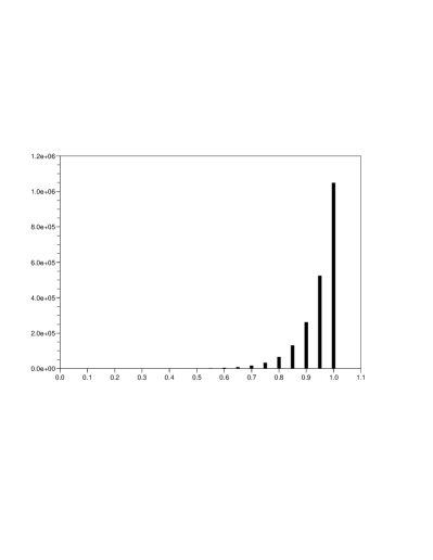
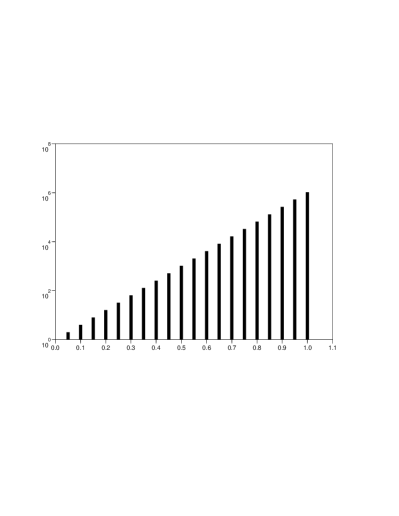
  Figure 1: Degeneracies of the energy levels for case 1, in semi-logarithmic representation for the second picture.

• In the second case we chose the same $v_{j}$’s, the same volume $n=2^{21}-2$ and we chose the degeneracies according two a multinomial law with parameters $n$, $1/20$, …, $1/20$. See Figure 2.

  

  

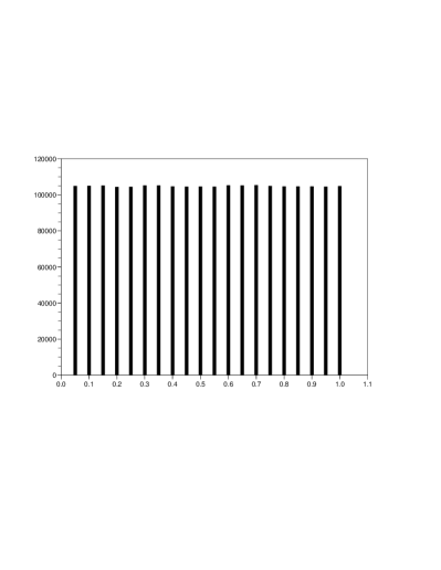
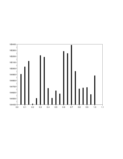
  Figure 2: Degeneracies of the energy levels for case 2, with shifted and rescaled axis for the second picture.

We were then interested in

$$d(t)=\max_{\eta\in{\cal X}_{k,m}}\|p^{t}(\eta_{0},\cdot)-\nu\|_{TV}=\max_{\eta\in{\cal X}_{k,m}}\frac{1}{2}\sum_{\eta\in{\cal X}_{k,m}}|p^{t}(\eta_{0},\eta)-\nu(\eta)|$$ (A.1)

for $t\geq 0$. The cardinality of ${\cal X}_{k,m}$ being very large (equal to $\binom{69}{19}\simeq 5\times 10^{16}$ in case 2), one faces three difficulties with such a formula:

• One cannot compute $\nu(\eta)$ and $p^{t}(\eta_{0},\eta)$ for given $\eta$ and $\eta_{0}$.

• The sum in (A.1) contained too many terms to be computed.

• It is not possible to try all the possible $\eta_{0}$ before taking the maximum in (A.1).

We addressed the first difficulty by replacing $p^{t}(\eta_{0},\cdot)$ by the empirical measure

$$\mu_{t}^{N}:=\frac{1}{N}\sum_{l=1}^{N}\delta_{X_{t}^{l}}$$ (A.2)

computed with a large number $N$ of simulated independent copies $(X_{t}^{l})_{t\in{\mathbb{N}}}$ of our Markov chain starting from $\eta_{0}$ and, using Theorem 1, by replacing $\nu$ by

$$\nu^{N}:=\frac{1}{2T}\sum_{t=T+1}^{2T}{\mu^{\prime}_{t}}^{N}+{\mu^{\prime\prime}_{t}}^{N}$$ (A.3)

with $T:=\lfloor km\ln(k/\epsilon)\rfloor$ and where ${\mu^{\prime}_{t}}^{N}$ and ${\mu^{\prime\prime}_{t}}^{N}$ are independently computed like $\mu_{t}^{N}$, starting from two different configurations. We addressed the second difficulty by looking at a coarse grained version $\bar{\cal X}_{k,m}$ of ${\cal X}_{k,m}$ through the free entropy $\phi$. More precisely, with $I^{N}=[\phi_{-},\phi_{+}]$ the smallest interval containing the support of $\phi(\nu^{N})=\nu^{N}\circ\phi^{-1}$ we divided $I^{N}$ into $M$ intervals of length $\Delta=(\phi_{+}-\phi_{-})/M$, we extended this partition of $I^{N}$ into a partition of ${\mathbb{R}}$ in intervals of length $\Delta$ and grouped in a same class the configurations $\eta\in{\cal X}_{k,m}$ that fall into a same interval. (For possible cases where $\phi_{-}=\phi_{+}$, we used a partition of ${\mathbb{R}}$ into intervals of length $10^{-6}$.) With $\bar{\phi}$ the canonical projection from ${\cal X}_{k,m}$ to $\bar{\cal X}_{k,m}$ we could then compute $\|\bar{\phi}(\mu_{t}^{N})-\bar{\phi}(\nu^{N})\|_{TV}$ rather than $\|\mu_{t}^{N}-\nu^{N}\|_{TV}$. Note that

$$\|\bar{\phi}(\mu_{t}^{N})-\bar{\phi}(\nu^{N})\|_{TV}\leq\|\mu_{t}^{N}-\nu^{N}\|_{TV},$$ (A.4)

and we also have, for large $M$ and as soon as $\phi$ is an injection from ${\cal X}_{k,m}$ to ${\mathbb{R}}$,

$$\|\mu_{t}^{N}-\nu^{N}\|_{TV}=\|\bar{\phi}(\mu_{t}^{N})-\bar{\phi}(\nu^{N})\|_{TV}+o(1).$$ (A.5)

As far as the third difficulty was concerned we underestimated

$$\bar{d}^{N}(t)=\max_{\eta_{0}\in{\cal X}_{k,m}}\|\bar{\phi}(\mu_{t}^{N})-\bar{\phi}(\nu^{N})\|_{TV}$$ (A.6)

by making a guess on a particular configuration $\eta_{0}$ for which $\|\bar{\phi}(\mu_{t}^{N})-\bar{\phi}(\nu^{N})\|_{TV}$ could be of the order of $\bar{d}^{N}(t)$. We simply took an $\eta_{0}$ for which we could have say, for all $\beta$, that it was “very far from typical configurations”. We first took $\eta_{0}=(0,\dots,0,k)$ since typical configurations are concentrated on the low energy levels when $\beta$ is large and have their occupation numbers $k_{j}$ distributed like the degeneracies $n_{j}$ when $\beta$ is small. Since this last point tends to show that in case 1 our specific $\eta_{0}$ is “not so far” from typical equilibrium configurations (we will come back on this point later), we also considered a different $\eta_{0}$, that one for which the high energy levels are empty and the low energy levels are saturated or as close to saturation as possible:

$$\eta_{0}=\left\{\begin{array}[]{ll}(2,4,8,16,20,0,\dots,0)&\mbox{in case 1,}\\ (50,0,\dots,0)&\mbox{in case 2.}\end{array}\right.$$ (A.7)

Then we simply took the maximum of the two quantities $\|\bar{\phi}(\mu_{t}^{N})-\bar{\phi}(\nu^{N})\|_{TV}$ computed, in each case, with these two specific choices.

Summing up, we approximated $d(t)$ by

$$\bar{d}_{0}^{N}(t)=\max_{\eta_{0}\in{\cal X}_{k,m}^{0}}\|\bar{\phi}(\mu_{t}^{N})-\bar{\phi}(\nu^{N})\|_{TV}$$ (A.8)

where ${\cal X}_{k,m}^{0}$ is the two configuration set described above. We chose $N=1024$ and $M=\sqrt{N}=32$ and we plotted for different temperatures a graphical representation of the law of $\bar{\phi}(\nu^{N})$ and the temporal evolution of $\bar{d}_{0}^{N}(t)$ for $0\leq t\leq 2T$. See Figures 3 to 7 for case 1 and Figures 8 to 12 for case 2.

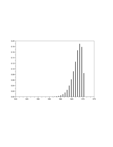
Figure 3: Probability distribution function of $\bar{\phi}(\nu^{N})$ and temporal evolution of $\bar{d}_{0}^{N}(t)$ for case 1 and $\beta=0$.

Figure 4: Probability distribution function of $\bar{\phi}(\nu^{N})$ and temporal evolution of $\bar{d}_{0}^{N}(t)$ for case 1 and $\beta=4$.

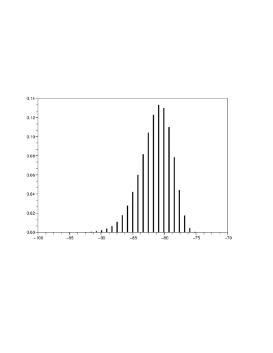
Figure 5: Probability distribution function of $\bar{\phi}(\nu^{N})$ and temporal evolution of $\bar{d}_{0}^{N}(t)$ for case 1 and $\beta=16$.

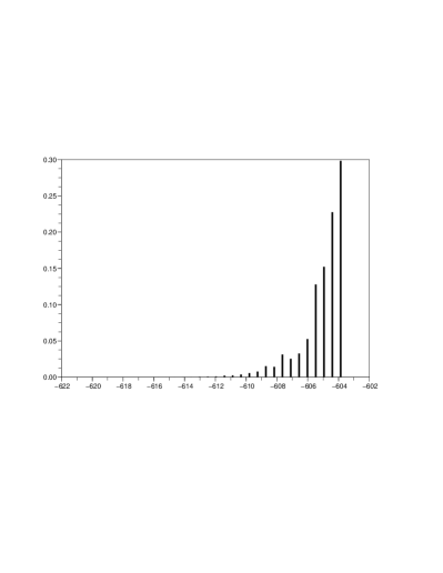
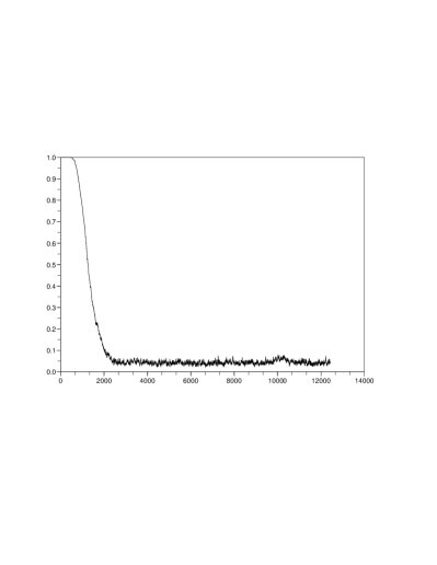
Figure 6: Probability distribution function of $\bar{\phi}(\nu^{N})$ and temporal evolution of $\bar{d}_{0}^{N}(t)$ for case 1 and $\beta=63$.

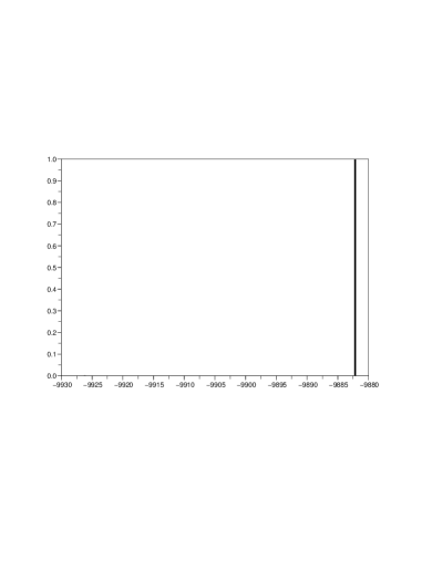
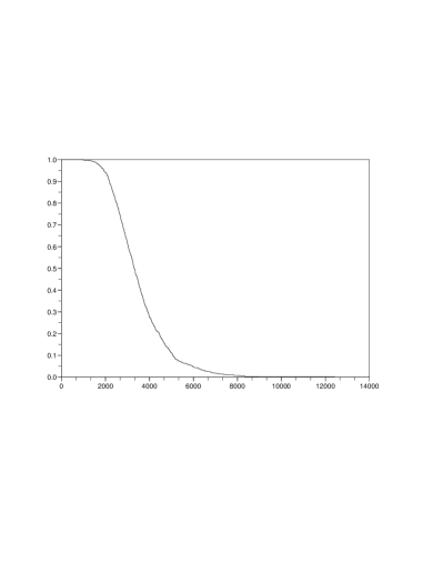
Figure 7: Probability distribution function of $\bar{\phi}(\nu^{N})$ and temporal evolution of $\bar{d}_{0}^{N}(t)$ for case 1 and $\beta=1000$.

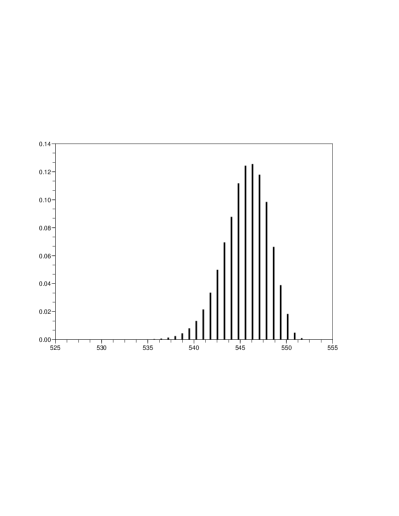
Figure 8: Probability distribution function of $\bar{\phi}(\nu^{N})$ and temporal evolution of $\bar{d}_{0}^{N}(t)$ for case 2 and $\beta=0$.

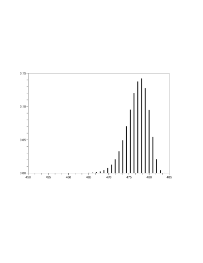
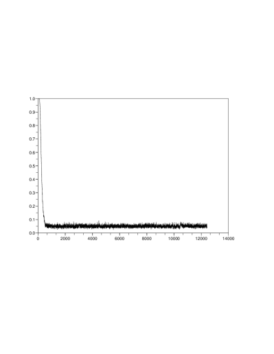
Figure 9: Probability distribution function of $\bar{\phi}(\nu^{N})$ and temporal evolution of $\bar{d}_{0}^{N}(t)$ for case 2 and $\beta=4$.

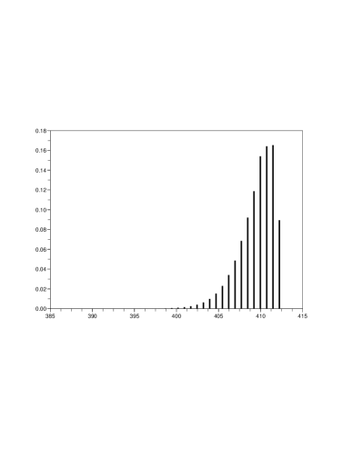
Figure 10: Probability distribution function of $\bar{\phi}(\nu^{N})$ and temporal evolution of $\bar{d}_{0}^{N}(t)$ for case 2 and $\beta=16$.

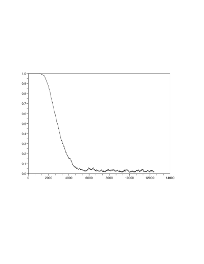
Figure 11: Probability distribution function of $\bar{\phi}(\nu^{N})$ and temporal evolution of $\bar{d}_{0}^{N}(t)$ for case 2 and $\beta=63$.

Figure 12: Probability distribution function of $\bar{\phi}(\nu^{N})$ and temporal evolution of $\bar{d}_{0}^{N}(t)$ for case 2 and $\beta=1000$.

For each temperature we get in each case an estimation $\hat{t}_{\epsilon}$ of $t_{\epsilon}$. Estimating $t_{\epsilon}$ in this way for 51 temperatures ($\beta=0$ included) we show in Figure 13 the graphical representations of the simulated dependency of $\hat{t}_{\epsilon}$ on $\beta>0$ together with our upper bound from Theorem 1.

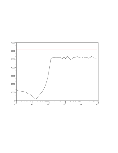
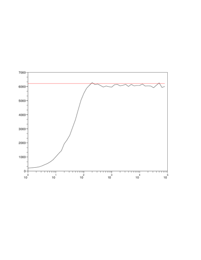
Figure 13: Dependency of $\hat{t}_{\epsilon}$ on $\beta$ in case 1 and 2 respectively (semi-logarithmic representation). The horizontal line stands for our theoretical upper bound.

We can now conclude with a few comments. First, with such a procedure, $t_{\epsilon}$ is essentially underestimated. Indeed, except for the replacement of $p^{t}(\eta_{0},\cdot)$ and $\nu$ by $\mu^{N}_{t}$ and $\nu^{N}$ our successive approximations underestimated $d(t)$ then $t_{\epsilon}$. As a consequence we recover with case 2 that $km\ln(k/\epsilon)$ is the best upper bound on $t_{\epsilon}$ that is uniform over the disorder.

Second, we note that $\beta$ can be seen as a tuning parameter for the disorder. We recover that our theoretical estimate on $t_{\epsilon}$ can be improved by a factor of order $m$ in weak disorder situations.

Last, it is worth to note that case 1 suggests that $t_{\epsilon}$ is not generally decreasing with the temperature. In our preliminary simulations we only considered $\eta_{0}=(0,\dots,0,50)$ to estimate the mixing time. Then we feared that our non monotonic estimation could be an artefact of our simulation. This led us to introduce the alternative saturated low level starting configuration, confirming in that way the non-monotonicity.

References

- [1] D. Bakry, M. Émery (1985) Diffusions hypercontractives, Séminaire de probabilités, XIX, 1983/84 Lecture Notes in Math., 1123, Springer, Berlin, 177–206.
- [2] R. Pemantle (1997) Towards a theory of negative dependence, J. Math. Phys. 41, 1371–1390.
- [3] T. M. Liggett (1997) Ultra logconcave sequences and negative dependence, J. Combin. Theory Ser. A 79, 315–325.
- [4] L. Saloff-Coste (1997) Lectures on finite Markov chains, in Lectures on probability theory and statistics, Saint-Flour 1996 Lecture Notes in Math., 1665, Springer, 301–413
- [5] C. Ané, S. Blachère, D. Chafaï, P. Fougères, I. Gentil, F. Malrieu, C. Roberto and G. Scheffer (2000) Sur les inégalités de Sobolev logarithmiques Panoramas et Synthèses no. 10, SMF, Paris.
- [6] P. Caputo (2004) Spectral gap inequalities in product spaces with conservation laws, in: T. Funaki and H. Osada (eds.) Adv. Studies in Pure Math.
- [7] C. Landim, J. Noronha Neto (2005) Poincaré and logarithmic Sobolev inequality for Ginzburg-Landau processes in random environment, Probab. Theory Related Fields 131, 229–260
- [8] A.S. Boudou, P. Caputo, P. Dai Pra, G. Posta (2006) Spectral gap inequalities for interacting particle systems via a Bochner type inequality, J. Funct. Anal. 232, 222–258.
- [9] R. Montenegro and P. Tetali (2006) Mathematical Aspects of Mixing Times in Markov Chains, Book in series Foundations and Trends in Theoretical Computer Science (ed: M. Sudan), vol. 1:3, NOW Publishers, Boston-Delft.
- [10] P. Caputo, P. Dai Pra, G. Posta (2007) Convex entropy decay via the Bochner-Bakry-Emery approach, Annales de l’Institut Henri Poincaré Probab. et Stat. (to appear), arXiv:0712.2578.
- [11] A. Iovanella, B. Scoppola, E. Scoppola (2007) Some spin glass ideas applied to the clique problem, Journal of Statistical Physics, 126, 895–915.
- [12] P. Caputo (2008) On the spectral gap of the Kac walk and other binary collision processes, ALEA, Latin American Journal Of Probability And Mathematical Statistics 4, 205–222.
- [13] O. Johnson (2008) Bounds on the Poincaré constant of ultra log-concave random variables, arXiv:0801.2112, preprint.
- [14] D.A. Levin, Y. Peres, E.L. Wilmer (2008) Markov Chains and mixing times, American Mathematical Society.
- [15] A. Joulin, Y. Ollivier (2009) Curvature, concentration, and error estimates for Markov chain Monte Carlo, The Annals of Probability (to appear) arXiv:0904.1312.