Dirac Fermions in Graphene Nanodisk and Graphene Corner:
Texture of Vortices with Unusual Winding Number

Abstract

We analyze the zero-energy sector of the trigonal zigzag nanodisk and corner based on the Dirac theory of graphene. The zero-energy states are shown to be indexed by the edge momentum and grouped according to the irreducible representation of the trigonal symmetry group $C_{3v}$. Wave functions are explicitly constructed as holomorphic or antiholomorphic functions around the K or K’ point. Each zero-energy mode is a chiral edge mode. We find a texture of magnetic vortices. It is intriguing that a vortex with the winding number $2$ emerges in the state belonging to the $E$ (doublet) representation. The realization of such a vortex is vary rare.

Graphene nanostructureGraphEx has opened a field of carbon-based nanoelectronics and spintronics alternative of silicon or GaAs. Carbon is a common material and ecological. Large spin relaxation length is ideal for spintronicsTombros . The basic graphene derivatives are nanoribbonsFujita96 ; EzawaRibbon ; Brey73 and nanodisksEzawaDisk ; Fernandez ; Hod ; Wang ; Potasz . They correspond to quantum wires and quantum dots, respectively. Regarding a nanodisk as a quantum dot with internal degrees of freedom, similar but richer physics and applications are anticipatedEzawaCouloKondoSpin . There are many type of nanodisks, among which the trigonal zigzag nanodisk [Fig.1] is prominent in its electronic and magnetic properties owing to the zero-energy sectorEzawaDisk . The main feature is that it becomes a quasiferromagnet in the presence of Coulomb interactionsEzawaDisk . Recently trigonal nanodisks have been experimentally obtained by way of the Ni etching of a graphene sheetNi . An experimental realization will undoubtedly accelerate further experimental and theoretical studies on graphene nanodisks.

In graphene, the physics of electrons near the Fermi energy is described by the massless two-component Dirac equation or the Weyl equationSlonczewski ; Semenoff ; Ajiki . Nanoribbons have been successfully analyzed based on the Weyl equationBrey73 , but this is not yet the case with respect to nanodisks. The Dirac theory of graphene nanodisks must be indispensable to explore deeper physics and promote further researches.

The carbon atoms form a honeycomb lattice in graphene. We take the basis vectors $\mathbf{a}_{1}=\left(1,0\right)a$ and $\mathbf{a}_{2}=(1/2,\sqrt{3}/2)a$ with $a$ the lattice constant ($a\approx 2.46$Å). The honeycomb lattice is bipartite and has two different atoms per primitive cell, which we call the A and B sites [Fig.1]. The Brillouin zone is a hexagon in the reciprocal lattice with opposite sides identified. We start with the tight-binding model (TBM) only with the nearest neighbor hopping $t$. We ignore the spin degree of freedom in most parts in what follows.

The band structure is such that the Fermi point is reached by six corners of the first Brillouin zone, among which there are only two inequivalent points. We call them the K and K’ points. The dispersion relation is linear around them, $E_{\kappa}\left(\mathbf{k}\right)\simeq\hbar v_{\text{F}}|\mathbf{k}-\mathbf{K}_{\tau}|$ with $\tau=\pm$, where $v_{\text{F}}=\sqrt{3}ta/2\hbar$ is the Fermi velocity and $\mathbf{K}_{\tau}=a^{-1}\left(\tau 2\pi/3,2\pi/\sqrt{3}\right)$ for the K point ($K_{+}$) and the K’ point ($K_{-}$).

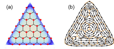
Figure 1: (Color on line) Trigonal zigzag graphene nanodisk. (a) The nanodisk size is defined by $N=N_{\text{ben}}-1$ with $N_{\text{ben}}$ the number of benzenes on one side of the trigon. Here, $N=5$. The A sites are indicated by red dots. The electron density is found to be localized along the edges. (b) A vortex texture emerges in the real-space Berry connection. In this example, the winding number is $2$ for the vortex at the center of mass while it is $1$ for all others.

The dispersion relation near the K and K’ points is that of ‘relativistic’ Dirac fermions. Indeed, the TBM yields the quantum-mechanical HamiltonianSlonczewski ; Semenoff ; Ajiki ,

$$H_{\tau}=\hbar v_{\text{F}}\left(\begin{array}[c]{cc}0&\tau\hat{k}_{x}-i\hat{k}_{y}\\ \tau\hat{k}_{x}+i\hat{k}_{y}&0\end{array}\right),$$ (1)

where we have introduced the reduced wave number by $\hat{\mathbf{k}}=\mathbf{k}-\boldsymbol{K}_{\tau}$. The Hamiltonian acts on the two-component envelope function, $\Phi_{\tau}=(\phi_{\text{A}}^{\tau},\phi_{\text{B}}^{\tau})$. Each Hamiltonian describes the two-component massless Dirac fermion or the Weyl fermion. The Weyl equations read

$$i\hbar\partial_{t}\Phi_{\tau}(\mathbf{x})=v_{\text{F}}\mathbf{\sigma}\cdot\mathbf{p}_{\tau}\Phi_{\tau}(\mathbf{x}),$$ (2)

where $\mathbf{p}_{\tau}=\hbar(\tau\hat{k}_{x},\hat{k}_{y})=-i\hbar(\tau\partial_{x},\partial_{y})$. The wave function is given by $\psi_{S}^{\tau}(\mathbf{x})=e^{i\boldsymbol{K}_{\tau}\cdot\boldsymbol{x}}\phi_{S}^{\tau}(\mathbf{x})$.

The symmetries are as follows. We note that $H_{\text{K'}}=\sigma_{y}H_{\text{K}}\sigma_{y}$ and $\sigma_{z}H_{\tau}\sigma_{z}=-H_{\tau}$, where $\sigma_{y}$ and $\sigma_{z}$ are the generators of the mirror symmetry and the electron-hole symmetry, respectively.

In terms of the complex variable, the Weyl equation reads

$$\partial_{z^{\ast}}\phi_{\text{A}}^{\text{K}}(\boldsymbol{x}) =i\varepsilon\phi_{\text{B}}^{\text{K}}(\boldsymbol{x}), \partial_{z}\phi_{\text{B}}^{\text{K}}(\boldsymbol{x}) =i\varepsilon\phi_{\text{A}}^{\text{K}}(\boldsymbol{x}),$$ (3a)

$$\partial_{z}\phi_{\text{A}}^{\text{K'}}(\boldsymbol{x}) =-i\varepsilon\phi_{\text{B}}^{\text{K'}}(\boldsymbol{x}), \partial_{z^{\ast}}\phi_{\text{B}}^{\text{K'}}(\boldsymbol{x}) =-i\varepsilon\phi_{\text{A}}^{\text{K'}}(\boldsymbol{x}),$$ (3b)

with $$\varepsilon=E/2\hbar v_{\text{F}} E=0$$. The envelope functions are holomorphic or antiholomorphic for the zero-energy state ().

Dirac electrons on zigzag edge: We analyze a graphene sheet placed in the upper half plane ($y\geq 0$) with the edge at $y=0$. Translational invariance in the $x$ direction dictates the envelope function is of the form $\phi_{S}^{\tau}(x,y)=e^{i\hat{k}_{x}x}f_{S}^{\tau}\left(y\right)$. Due to the analyticity requirement we obtain

$$\phi_{\text{A}}^{\text{K}}(\boldsymbol{x}) =C_{\text{A}}^{\text{K}}e^{i\hat{k}(x+iy)}, \phi_{\text{B}}^{\text{K}}(\boldsymbol{x}) =C_{\text{B}}^{\text{K}}e^{i\hat{k}(x-iy)},$$ (4a)

$$\phi_{\text{A}}^{\text{K'}}(\boldsymbol{x}) =C_{\text{A}}^{\text{K'}}e^{i\hat{k}(x-iy)}, \phi_{\text{B}}^{\text{K'}}(\boldsymbol{x}) =C_{\text{B}}^{\text{K'}}e^{i\hat{k}(x+iy)},$$ (4b)

with $$C_{S}^{\tau}$$ being normalization constants. Hereafter we ignore such normalization constants.

According to the TBM result, there are no electrons in the B site on edges. Hence we require $\phi_{\text{B}}^{\tau}\left(y=0\right)=0$. By avoiding divergence at $y\rightarrow\infty$, the resultant envelope functions are found to be $\phi_{\text{A}}^{\text{K}}(\boldsymbol{x})=e^{i\hat{k}z}$ for $\hat{k}>0$ and $\phi_{\text{A}}^{\text{K'}}(\boldsymbol{x})=e^{i\hat{k}z^{\ast}}$ for $\hat{k}<0$, with all other components being zero.

The wave number is a continuous parameter for an infinitely long graphene edge. According to the TBM result, the flat band emerges for

$$-\pi\leq ak<-2\pi/3\quad\text{and}\quad 2\pi/3<ak\leq\pi,$$ (5)

around the K’ and K points, respectively. The boundary points $ak=-\pi$ and $ak=\pi$ are to be identified since they represent the same point in the Brillouin zone.

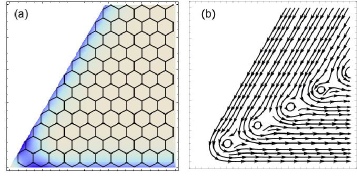
Figure 2: (Color on line) (a) Trigonal corner of graphene. The electron density is found to be localized along the edges. (b) Real-space Berry connection for the trigonal corner. A series of vortices are found to be present.

Dirac electrons in trigonal corner: We apply the above analysis to the study of the envelope functions for electrons in the zero-energy sector of the zigzag trigonal corner [Fig.2(a)], which is an infinite region surrounded by the $x$ axis and the line with the angle $\arg z=\pi/3$. They are holomorphic (antiholomorphic) around the K (K’) point. Here we discuss envelope functions around the K point. We start with the solution $\phi_{1}\left(z\right)=Ce^{i\hat{k}z}$ for the upper half plane. We rotate this by the angle $\pi/3$, which presents us with the solution $\phi_{2}\left(z\right)=Ce^{i\hat{k}z\exp\left[2\pi i/3\right]}$ for another half plane. The trigonal corner is given by the overlap region of these two half planes, which is described by a linear combination of these two functions with an appropriate coefficient. It is to be fixed by imposing the boundary condition: Since the top of the corner is located at $z=0$, where there is no atom, we impose $\phi_{\text{A}}^{\text{K}}(0)=0$. The resultant function is $\phi_{\text{A}}^{\text{K}}(\mathbf{x})=\phi\left(z\right)$ with

$$\phi\left(z\right)=e^{i\hat{k}z}-e^{i\hat{k}z\exp\left[2\pi i/3\right]}.$$ (6)

The phase shift is $\pi$ at the corner. The envelope function around the K’ point ($\hat{k}<0$) is given by $\phi_{\text{A}}^{\text{K'}}(\mathbf{x})=\phi\left(z^{\ast}\right)$.

We calculate the real-space Berry connection, $\mathcal{A}_{i}(\mathbf{x})=-i\left\langle\phi\right|\partial_{i}\left|\phi\right\rangle$. It exhibits a series of vortices [Fig.2(b)], where the wave function vanishes. It has an infinite number of zero points at $z_{n}=(2\pi n/\sqrt{3}\hat{k})e^{\pi i/6}$, $n=1,2,3,\cdots$, around which it is expanded as $\phi\left(z\right)=\hat{k}(z-z_{n})$.

Dirac electrons in trigonal nanodisk: Our main purpose is to apply the above result to the analysis of the zero-energy sector of the trigonal zigzag nanodisk [Fig.1]. The envelope function of the trigonal zigzag nanodisk can be constructed by making a linear combination of envelope functions for three trigonal corners. We consider the trigonal region whose corners are located at $z_{1}=\left(L,0\right)$, $z_{2}=\left(-L,0\right)$, $z_{3}=\left(0,\sqrt{3}L\right)$. As the boundary conditions we impose $\phi\left(z_{1}\right)=\phi\left(z_{2}\right)=\phi\left(z_{3}\right)=0$. The envelope function is obtained around the K point ($\hat{k}>0$) as $\phi_{\text{A}}^{\text{K}}(\mathbf{x})=\phi\left(z\right)$ with

$$\phi\left(z\right) =e^{i\hat{k}z}-e^{i\hat{k}L}e^{i\hat{k}\left(z-L\right)\exp\left[-2\pi i/3\right]}$$

$$-e^{-i\hat{k}L}e^{i\hat{k}\left(z+L\right)\exp\left[2\pi i/3\right]}.$$ (7)

The envelope function around the K’ point ($\hat{k}<0$) is given by $\phi_{\text{A}}^{\text{K'}}(\mathbf{x})=\phi\left(z^{\ast}\right)$. Note that $\phi_{\text{B}}^{\tau}(\mathbf{x})=0$ identically, as is consistent with the TBM resultEzawaDisk .

The wave number is quantized for a finite edge such as in the trigonal nanodisk. We focus on the wave function $\psi_{\text{A}}^{\tau}\left(\mathbf{x}\right)$ at one of the A sites on an edge. For definiteness let us take it on the $x$-axis. We investigate the phase shift between two points $(x,0)$ and $(x+ma,0)$,

$$\Theta^{\tau}(x,m)=\tau\frac{2\pi m}{3}+\arg\phi\left(x+ma\right)-\arg\phi\left(x\right),$$ (8)

with (7). There are $N$ links along one edge of the size-$N$ nanodisk, for which we obtain precisely $\Theta^{\tau}(a/2,N)=Nak$. On the other hand, the phase shift is $\pi$ at the corner. The total phase shift is $3Nak+3\pi$, when we encircle the nanodisk once. This phase shift agrees with the TBM result. By requiring the single-valueness of the wave function, and taking into account the allowed region of the wave number (5), we find that the wave number is quantized as

$$ak_{n}=\pm\left[(2n+1)/3N+2/3\right]\pi,\quad 0\leq n\leq(N-1)/2.$$ (9)

When $N$ is even, there are $N/2$ states for $k_{n}>0$ and $N/2$ states $k_{n}<0$. When $N$ is odd, there are $(N-1)/2$ states for $k_{n}>0$ and $(N-1)/2$ states for $k_{n}<0$. Additionally, there seem to appear two modes with $ak_{n}=\pm\pi$ at $n=(N-1)/2$. However, they are identified with one another, since they are located at the boundary of the Brillouin zone. There are $N$ states in both of the cases, as agrees with the TBM resultEzawaDisk .

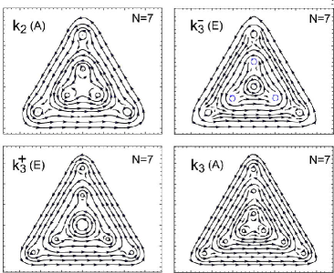
Figure 3: Vortex textures in the real-space Berry connection for the state $|k_{n}^{\alpha}\rangle$ in the nanodisk with $N=7$. The representation is indicated in the parenthesis. There are $n$ vortices along the $y$-axis in $|k_{n}^{\alpha}\rangle$. A vortex appears at the center of mass for the $E$-mode $|k_{n}^{\pm}\rangle$. It is interesting that the winding number is $2$ in the state $|k_{n}^{+}\rangle$.

Trigonal symmetry group: The symmetry group of the trigonal nanodisk is $C_{3v}$, which is generated by the $2\pi/3$ rotation $\mathfrak{c}_{3}$ and the mirror reflection $\sigma_{v}$. It has the irreducible representation {$A_{1}$, $A_{2}$, $E$}. The $A_{1}$ representation is invariant under the rotation $\mathfrak{c}_{3}$ and the mirror reflection $\sigma_{v}$. The $A_{2}$ representation is invariant under $\mathfrak{c}_{3}$ and antisymmetric under $\sigma_{v}$. The $E$ representation acquires $\pm 2\pi/3$ phase shift under the $2\pi/3$ rotation. The $A_{1}$ and $A_{2}$ are 1-dimensional representations (singlets) and the $E$ is a 2-dimensitional representation (doublet). These properties are summarized in the following character table.

$$\begin{array}[c]{c|ccc}\hline\cr C_{3v}&\mathfrak{e}&2\mathfrak{c}_{3}&3\sigma_{v}\\ \hline\cr A_{1}&1&1&1\\ A_{2}&1&1&-1\\ E&2&-1&0\\ \hline\cr\end{array}$$ (10)

The mirror symmetry is equivalent to the exchange of the K and K’ points. With respect to the rotation there are three elements $\mathfrak{c}_{3}^{0}$, $\mathfrak{c}_{3}$, $\mathfrak{c}_{3}^{2}$, which correspond to $1$, $e^{2\pi i/3}$, $e^{4\pi i/3}$. Accordingly, the phase shift of one edge is $0$, $2\pi/3$, $4\pi/3$. From this requirement we deduce that the state, indexed by the edge momentum $k_{n}$ as in (9), is grouped according to the representation of the symmetry group $C_{3v}$ as follows,

$$\begin{array}[c]{cc}\left.\begin{array}[c]{cc}A_{1}\text{ (singlet)}:&|k_{n}^{0}\rangle+|-k_{n}^{0}\rangle,\\ A_{2}\text{ (singlet)}:&|k_{n}^{0}\rangle-|-k_{n}^{0}\rangle,\end{array}\right\}&\displaystyle k_{n}^{0}=\frac{6n+3}{3Na}\pi,\\ \begin{array}[c]{cc}E\text{ (doublet)}:&|k_{n}^{\pm}\rangle,\quad|-k_{n}^{\pm}\rangle,\end{array}&\displaystyle k_{n}^{\pm}=\frac{6n\pm 1}{3Na}\pi,\end{array}$$ (11)

where $k_{n}^{\alpha}$ is subject to the condition (5). It follows that

$$\left\lfloor(N+1)/3\right\rfloor\leq n\leq\left\lfloor N/2\right\rfloor,$$ (12)

where $\left\lfloor a\right\rfloor$ denotes the maximum integer equal to or smaller than $a$. Some examples read

$$\begin{array}[c]{c|c|c|c|c|c}N&3&4&5&6&7\\ \hline\cr A_{1}&&k_{1}^{0}&&k_{2}^{0}&k_{2}^{0}\\ \hline\cr A_{2}&k_{1}^{0}&k_{1}^{0}&k_{2}^{0}&k_{2}^{0}&k_{2}^{0},k_{3}^{0}\\ \hline\cr E&\pm k_{1}^{+}&\pm k_{2}^{-}&\pm k_{2}^{-},\pm k_{2}^{+}&\pm k_{2}^{+},\pm k_{3}^{-}&\pm k_{3}^{-},\pm k_{3}^{+}\end{array}$$ (13)

The numbers of doublets ($E$-mode) and singlets ($A_{i}$-mode) are given by $\left\lfloor\frac{1}{3}(N+1)\right\rfloor$ and $N-2\left\lfloor\frac{1}{3}(N+1)\right\rfloor$, respectively.

Berry connection: To see the meaning of the wave number $k_{n}^{\alpha}$ more in detail, we have calculated the Berry connection for various states, which we show for the case of $N=7$ in Fig.3. Each mode is found to be chiral. We observe clearly a texture of vortices: The number of vortices is $6,7,7,9$ for $|k_{2}^{0}\rangle$, $|k_{3}^{-}\rangle$, $|k_{3}^{+}\rangle$, $|k_{3}^{0}\rangle$, respectively. The vortex at the center of mass has the winding number $2$ in $|k_{3}^{+}\rangle$. In general, the total winding number $N_{\text{vortex}}$ is calculated by

$$N_{\text{vortex}}=\frac{-i}{2\pi}{\displaystyle\oint}dx_{i}\,\frac{\phi^{\ast}(x,y)\partial_{i}\phi(x,y)}{|\phi(x,y)|^{2}}=N+m-1,$$ (14)

with $m=0,1,2,\cdots,\left\lfloor(N-1)/2\right\rfloor$ in the size-$N$ nanodisk, where the integration is made along the closed edge of a nanodisk. There are $n$ vortices along the $y$-axis in the state $|k_{n}^{\alpha}\rangle$. The state $|k_{n}^{\pm}\rangle$, being the $E$-mode, has a vortex at the center of mass, where the winding number is $2$ in the state $|k_{n}^{+}\rangle$. On the other hand, the state $|k_{n}^{0}\rangle$ does not have a vortex at the center of mass, and the combinations $|k_{n}^{0}\rangle\pm|-k_{n}^{0}\rangle$ belong to the A₁ and A₂ representations, respectively. This statement is demonstrated by investigating the zero points of the envelop function (7), where vortices appear. For instance, it is expanded around the center of mass $z=z_{0}$ as $\psi\left(z\right)=\sum_{n=0}C_{n}(z-z_{0})^{n}$, where the coefficients $C_{0}$ and $C_{1}$ are found to vanish at $k=k_{n}^{\pm}$ and $k=k_{n}^{+}$, respectively, with $C_{3}\neq 0$. Hence the winding number is $2$ for $k=k_{n}^{+}$.

It should be emphasized that there exists a good agreement with respect to the edge states between the Dirac description and the exact diagonalization results of the TBM even for a small system. Indeed, we can easily compute the phase at each lattice point by exact numerical methods. Then, comparing it with the result due to the Dirac description, it is easy to see that a good agreement holds between them. This shows that the real space Barry connection computed by exact numerical methods has the same physical reality with the one obtained by using the Dirac Hamiltonian.

Zero-energy splitting due to Coulomb interactions: We have constructed explicitly the wave function for each state in the size-$N$ trigonal nanodisk. All these states are edge modes belonging to the zero-energy sector. When Coulomb interactions are taken into account, the degeneracy among the zero-energy states is resolvedEzawaDisk . The Coulomb Hamiltonian has the trigonal symmetry $C_{3v}$, and the energy spectrum splits into different levels according to its representation, as illustrated in Fig.4.

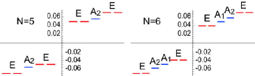
Figure 4: (Color on line) The energy spectrum with Coulomb interactions in nanodisks with $N=5,6$, derived based on the tight-bindind model. The vertical axis stands for the energy in unit of $1$eV. The $N$-folded degenerate states in the noninteraction regime split into different levels according to the representation of the trigonal symmetry $C_{3v}$, as indicated. For instance, the positive (negative) energy levels are for down-spin (up-spin) states. The ground state is a ferromagnet.

There exists additionally the spin degeneracy in the noninteracting Hamiltonian: The total degeneracy is $2N$. The spin degeneracy is broken spontaneously due to the exchange interaction when Coulomb interactions are introducedEzawaDisk . The splitting is symmetric with respect to the zero-energy level. At half-filling, electrons with the identical spin fill all energy levels under the Fermi energy. Then, the spin of the ground state is $N/2$, and it is a ferromagnet. We show the energy spectrum for $N=5,6$ in Fig.4. By tuning the chemical potential any of them is made the ground state.

Magnetic vortices: The zero-energy degeneracy is resolved by the Coulomb interaction, and the dispersion relation becomes nontrivial. The time-dependent solution is well known,

$$\psi_{\text{A}}^{\text{K}}(t,\boldsymbol{x})= e^{-i(E_{n}^{\alpha}t-k_{n}^{\alpha}x)-k_{n}^{\alpha}y},$$ (15a)

$$\psi_{\text{A}}^{\text{K'}}(t,\boldsymbol{x})= e^{-i(E_{n}^{\alpha}t+k_{n}^{\alpha}x)-k_{n}^{\alpha}y},$$ (15b)

where $$E_{n}^{\alpha} |k_{n}^{\alpha}\rangle A_{i} |k_{n}^{0}\rangle\pm|-k_{n}^{0}\rangle E |k_{n}^{\beta}\rangle |-k_{n}^{\beta}\rangle \beta=\pm$$ is the energy of the state [Fig.4]. Here we have suppressed the spinor part. On one hand, the -modes represent standing waves. On the other hand, the -modes and represent the right-propagating mode and the left-propagating mode, respectively, for .

Charged particles propagating along a closed edge generates magnetic field. The electromagnetic interaction is described in terms of the electromagnetic potential $\mathbf{A}$, which is introduced to the system by way of the Peierls substitution $\partial_{j}\rightarrow\partial_{j}+ieA_{j}/\hbar$. From the Weyl equation (3) we derive

$$eA_{i}(\boldsymbol{x})=\hbar\mathcal{A}_{i}(\boldsymbol{x})/|\phi_{\text{A}}^{\text{K}}(\boldsymbol{x})|^{2}$$ (16)

with $\mathcal{A}_{i}(x,y)=-i\phi_{\text{A}}^{\text{K}\ast}(\mathbf{x})\partial_{i}\phi_{\text{A}}^{\text{K}}(\mathbf{x})$ in the lowest order of approximation, where $\phi_{\text{A}}^{\text{K}}(\mathbf{x})$ is assumed to be not modified from (7). The potential $A_{i}(\boldsymbol{x})$ exhibits the same texture of vortices as in Fig.3. The magnetic field is given by

$$B(\boldsymbol{x})=\nabla\times\mathbf{A}(\boldsymbol{x})=\frac{2\pi\hbar}{e}\sum_{n}\nu_{n}\delta\left(z-z_{n}\right),$$ (17)

where $\nu_{n}$ stands for winding number of the vortex at $z=z_{n}$. Hence a texture of vortices in the Berry connection leads to a texture of magnetic vortices. A comment is in order. This $\delta$-function type magnetic field would be smoothed out in a rigorous analysis of the coupled system of the Maxwell equation and the Weyl equation.

It is intriguing that, by tuning the chemical potential, a vortex with the winding number $2$ emerges in the ground state $|k_{n}^{+}\rangle$. As is well known, a single flux quantum has experimentally been observed in superconductor by using an electron-holographic interferometryTonomura . Then, in principle it is possible to observe a vortex texture in nanodisk as well. Furthermore, by attaching a superconductor film one may observe a disintegration of a vortex into two when the flux enters into the superconductor from the nanodisk. This would verify the winding number 2 of a vortex.

Conclusions: In this paper we have classified the zero-energy sector of the trigonal zigzag nanodisk into a fine structure according to the trigonal symmetry group $C_{3v}$. We have explicitly constructed wave functions based on the Dirac theory and specified them by the quantized edge momentum. A texture of magnetic vortices is found to emerge, which has an unusual winding number. As far as we are aware of, the vortex with the winding number 2 has never been found in all branches of physics. This is because two vortices with the winding number 1 have lower energy than one vortex with the winding number 2 in general. In the present case the disintegration of a vortex into two is prohibited by the trigonal symmetry.

I am very much grateful to Professors N. Nagaosa and H. Tsunetsugu for fruitful discussions on the subject and reading through the manuscript. This work was supported in part by Grants-in-Aid for Scientific Research from the Ministry of Education, Science, Sports and Culture No. 20940011.

References

(1)K. S. Novoselov, et al., Science 306, 666
(2004). K. S. Novoselov, et al., Nature 438, 197 (2005). Y.
Zhang, et al., Nature 438, 201 (2005).
(2)N. Tombros, et al., Nature 448, 571 (2007).
(3)M. Fujita, et al., J. Phys. Soc. Jpn. 65,
1920 (1996).
(4)M. Ezawa, Phys. Rev. B, 73, 045432 (2006).
(5)L. Brey, and H. A. Fertig, Phys. Rev. B, 73, 235411 (2006).
(6)M. Ezawa, Phys. Rev. B 76, 245415 (2007): M.
Ezawa, Physica E 40, 1421-1423 (2008): M. Ezawa, New J. Phys. 11,
095005 (2009).
(7)J. Fernández-Rossier, and J. J. Palacios, Phys. Rev.
Lett. 99, 177204 (2007).
(8)O. Hod, V. Barone, and G. E. Scuseria, Phys. Rev. B 77,
035411 (2008).
(9)W. L. Wang, S. Meng and E. Kaxiras, Nano Letters 8,
241 (2008).
(10)P. Potasz, A. D. Güçlü and P. Hawrylak, Phys.
Rev. B 81, 033403 (2010).
(11)L.C. Campos et al., Nano Lett., 9, 2600 (2009).
(12)M. Ezawa, Phys. Rev. B 77, 155411
(2008); ibid. B 79, 241407(R) (2009): M. Ezawa, Eur. Phys.
J. B 67, 543 (2009)
(13)J.C. Slonczewski and P.R. Weiss, Phys. Rev.
109, 272 (1958).
(14)G. W. Semenoff, Phys. Rev. Lett. 53, 2449 (1984).
(15)H. Ajiki and T. Ando, J. Phys. Soc. Jpn., 62, 1255
(1993); T. Ando, Y. Zheng and H. Suzuura, Microelectron. Eng., 63,
167 (2002).
(16)T. Matsuda, et al., Phys. Rev. Lett. 62,
2519 (1989).