Improving the Convergence Properties of the Data Augmentation Algorithm with an Application to Bayesian Mixture Modeling

Abstract

The reversible Markov chains that drive the data augmentation (DA) and sandwich algorithms define self-adjoint operators whose spectra encode the convergence properties of the algorithms. When the target distribution has uncountable support, as is nearly always the case in practice, it is generally quite difficult to get a handle on these spectra. We show that, if the augmentation space is finite, then (under regularity conditions) the operators defined by the DA and sandwich chains are compact, and the spectra are finite subsets of $[0,1)$. Moreover, we prove that the spectrum of the sandwich operator dominates the spectrum of the DA operator in the sense that the ordered elements of the former are all less than or equal to the corresponding elements of the latter. As a concrete example, we study a widely used DA algorithm for the exploration of posterior densities associated with Bayesian mixture models [J. Roy. Statist. Soc. Ser. B 56 (1994) 363–375]. In particular, we compare this mixture DA algorithm with an alternative algorithm proposed by Frühwirth-Schnatter [J. Amer. Statist. Assoc. 96 (2001) 194–209] that is based on random label switching.

, and

1 Introduction

Suppose that $f_{X}\dvtx\mathbb{R}^{p}\rightarrow[0,\infty)$ is a probability density function that is intractable in the sense that expectations with respect to $f_{X}$ cannot be computed analytically. If direct simulation from $f_{X}$ is infeasible, then classical Monte Carlo methods cannot be used to explore $f_{X}$ and one might resort to a Markov chain Monte Carlo (MCMC) method such as the data augmentation (DA) algorithm (Tanner and Wong, 1987; Liu, Wong and Kong, 1994; Hobert, 2011). To build a DA algorithm, one must identify a joint density, say, $f\dvtx\mathbb{R}^{p}\times\mathbb{R}^{q}\rightarrow[0,\infty)$, that satisfies two conditions: (i) the $x$-marginal of $f(x,y)$ is $f_{X}$, and (ii) sampling from the associated conditional densities, $f_{X|Y}(\cdot|y)$ and $f_{Y|X}(\cdot|x)$, is straightforward. (The $y$-coordinate may be discrete or continuous.) The first of the two conditions allows us to construct a Markov chain having $f_{X}$ as an invariant density, and the second ensures that we are able to simulate this chain. Indeed, let $\{X_{n}\}_{n=0}^{\infty}$ be a Markov chain whose dynamics are defined (implicitly) through the following two-step procedure for moving from the current state, $X_{n}=x$, to $X_{n+1}$ (see Procedure 1).

It is well known and easy to establish that the DA Markov chain is reversible with respect to $f_{X}$, and this of course implies that $f_{X}$ is an invariant density (Liu, Wong and Kong, 1994). Consequently, if the chain satisfies the usual regularity conditions (see Section 2), then we can use averages to consistently estimate intractable expectations with respect to $f_{X}$ (Tierney, 1994). The resulting MCMC algorithm is known as a DA algorithm for $f_{X}$. (Throughout this section, $f_{X}$ is assumed to be a probability density function, but, starting in Section 2, a more general version of the problem is considered.)

Procedure 1: Iteration $n+1$ of the DA Algorithm

[2.] 1. Draw $Y\sim f_{Y|X}(\cdot|x)$, and call the observed value $y$. 2. Draw $X_{n+1}\sim f_{X|Y}(\cdot|y)$.

When designing a DA algorithm, one is free to choose any joint density that satisfies conditions (i) and (ii). Obviously, different joint densities will yield different DA chains, and the goal is to find a joint density whose DA chain has good convergence properties. (This is formalized in Section 3 using $\chi^{2}$-distance to stationarity.) Unfortunately, the “ideal” joint density, which yields the DA chain with the fastest possible rate of convergence, does not satisfy the simulation requirement. Indeed, consider $f_{\perp}(x,y)=f_{X}(x)g_{Y}(y)$, where $g_{Y}(y)$ is any density function on $\mathbb{R}^{q}$. Since $f_{\perp}(x,y)$ factors, $f_{X|Y}(x|y)=f_{X}(x)$ and it follows that the DA chain is just an i.i.d. sequence from $f_{X}$. Of course, this ideal DA algorithm is useless from a practical standpoint because, in order to simulate the chain, we must draw from $f_{X}$, which is impossible. We return to this example later in this section.

It is important to keep in mind that there is no inherent interest in the joint density $f(x,y)$. It is merely a tool that facilitates exploration of the target density, $f_{X}(x)$. This is the reason why the DA chain does not possess a $y$-coordinate. In contrast, the two-variable Gibbs sampler based on $f_{X|Y}(\cdot|y)$ and $f_{Y|X}(\cdot|x)$, which is used to explore $f(x,y)$, has both $x$ and $y$-coordinates. So, while the two-step procedure described above can be used to simulate both the DA and Gibbs chains, there is one key difference. When simulating the DA chain, we do not keep track of the $y$-coordinate.

Every reversible Markov chain defines a self-adjoint operator whose spectrum encodes the convergence properties of the chain (Mira and Geyer, 1999; Rosenthal, 2003; Diaconis, Khare and Saloff-Coste, 2008). Let $X\sim f_{X}$ and consider the space of functions $g$ such that the random variable $g(X)$ has finite variance and mean zero. To be more precise, define

$$L^{2}_{0}(f_{X})=\biggl{\{}g\dvtx\mathbb{R}^{p}\rightarrow\mathbb{R}\dvtx\int_{\mathbb{R}^{p}}g^{2}(x)f_{X}(x)\,dx<\infty\mbox{ and }\int_{\mathbb{R}^{p}}g(x)f_{X}(x)\,dx=0\biggr{\}}.$$

Let $k(x^{\prime}|x)$ be the Markov transition density (Mtd) of the DA chain. (See Section 3 for a formal definition.) This Mtd defines an operator, $K\dvtx L^{2}_{0}\rightarrow L^{2}_{0}$, that maps $g(x)$ to

$$(Kg)(x):=\int_{\mathbb{R}^{p}}g(x^{\prime})k(x^{\prime}|x)\,dx^{\prime}.$$

Of course, $(Kg)(x)$ is just the expected value of $g(X_{1})$ given that $X_{0}=x$. Let $I\dvtx L^{2}_{0}\rightarrow L^{2}_{0}$ denote the identity operator, which leaves functions unaltered, and consider the operator $K-\lambda I$, where $\lambda\in\mathbb{R}$. By definition, $K-\lambda I$ is invertible if, for each $h\in L^{2}_{0}$, there exists a unique $g\in L^{2}_{0}$ such that $((K-\lambda I)g)(x)=(Kg)(x)-\lambda g(x)=h(x)$. The spectrum of $K$, which we denote by $\operatorname{Sp}(K)$, is simply the set of $\lambda$ such that $K-\lambda I$ is not invertible. Because $K$ is defined through a DA chain, $\operatorname{Sp}(K)\subseteq[0,1]$ (see Section 3). The number of elements in $\operatorname{Sp}(K)$ may be finite, countably infinite or uncountable.

In order to understand what “good” spectra look like, consider the ideal DA algorithm introduced earlier. Let $k_{\perp}$ and $K_{\perp}$ denote the Mtd and the corresponding operator, respectively. In the ideal case, $X_{n+1}$ is independent of $X_{n}$ and has density $f_{X}$. Therefore, the Mtd is just $k_{\perp}(x^{\prime}|x)=f_{X}(x^{\prime})$ and

$$(K_{\perp}g)(x)=\int_{\mathbb{R}^{p}}g(x^{\prime})f_{X}(x^{\prime})\,dx^{\prime}=0,$$

which implies that

$$\bigl{(}(K_{\perp}-\lambda I)g\bigr{)}(x)=-\lambda g(x).$$

It follows that $K_{\perp}\,{-}\,\lambda I$ is invertible as long as $\lambda\,{\neq}\,0$. Hence, the “ideal spectrum” is $\operatorname{Sp}(K_{\perp})=\{0\}$. Loosely speaking, the closer $\operatorname{Sp}(K)$ is to $\{0\}$, the faster the DA algorithm converges (Diaconis, Khare and Saloff-Coste, 2008).

Unfortunately, in general, there is no simple method for calculating $\operatorname{Sp}(K)$. Even getting a handle on $\operatorname{Sp}(K)$ is currently difficult. However, there is one situation where $\operatorname{Sp}(K)$ has a very simple structure. Let ${\mathsf{Y}}=\{y\in\mathbb{R}^{q}\dvtx f_{Y}(y)>0\}$, where $f_{Y}(y)=\int_{\mathbb{R}^{p}}f(x,y)\,dx$. We show that when ${\mathsf{Y}}$ is a finite set, $\operatorname{Sp}(K)$ consists of a finite number of elements that are directly related to the Markov transition matrix (Mtm) of the so-called conjugate chain, which is the reversible Markov chain that lives on ${\mathsf{Y}}$ and makes the transition $y\rightarrow y^{\prime}$ with probability $\int_{\mathbb{R}^{p}}f_{Y|X}(y^{\prime}|x)f_{X|Y}(x|y)\,dx$. In particular, we prove that when $|{\mathsf{Y}}|=d<\infty$, $\operatorname{Sp}(K)$ consists of the point $\{0\}$ together with the $d-1$ smallest eigenvalues of the Mtm of the conjugate chain. We use this result to prove that the spectrum associated with a particular alternative to the DA chain is closer than $\operatorname{Sp}(K)$ to the ideal spectrum, $\{0\}$.

Procedure 2: Iteration $n+1$ of the Sandwich Algorithm

[3.] 1. Draw $Y\sim f_{Y|X}(\cdot|x)$, and call the observed value $y$. 2. Draw $Y^{\prime}\sim r(\cdot|y)$, and call the observed value $y^{\prime}$. 3. Draw $\tilde{X}_{n+1}\sim f_{X|Y}(\cdot|y^{\prime})$.

DA algorithms often suffer from slow convergence, which is not surprising given the close connection between DA and the notoriously slow to converge EM algorithm (see, e.g., van Dyk and Meng, 2001). Over the last decade, a great deal of effort has gone into modifying the DA algorithm to speed convergence. See, for example, Meng and van Dyk (1999), Liu and Wu (1999), Liu and Sabatti (2000), van Dyk and Meng (2001), Papaspiliopoulos, Roberts and Sköld (2007), Hobert and Marchev (2008) and Yu and Meng (2011). In this paper we focus on the so-called sandwich algorithm, which is a simple alternative to the DA algorithm that often converges much faster. Let $r(y^{\prime}|y)$ be an auxiliary Mtd (or Mtm) that is reversible with respect to $f_{Y}$, and consider a new Markov chain, $\{\tilde{X}_{n}\}_{n=0}^{\infty}$, that moves from $\tilde{X}_{n}=x$ to $\tilde{X}_{n+1}$ via the following three-step procedure (see Procedure 2).

A routine calculation shows that the sandwich chain remains reversible with respect to $f_{X}$, so it is a viable alternative to the DA chain. The name “sandwich algorithm” was coined by Yu and Meng (2011) and is based on the fact that the extra draw from $r(\cdot|y)$ is sandwiched between the two steps of the DA algorithm. Clearly, on a per iteration basis, it is more expensive to simulate the sandwich chain. However, it is often possible to find an $r$ that leads to a substantial improvement in mixing despite the fact that it only provides a low-dimensional (and hence inexpensive) perturbation on the ${\mathsf{Y}}$ space. In fact, the computational cost of drawing from $r$ is often negligible relative to the cost of drawing from $f_{Y|X}(\cdot|x)$ and $f_{X|Y}(\cdot|y)$. Concrete examples can be found in Meng and van Dyk (1999), Liu and Wu (1999), van Dyk and Meng (2001), Roy and Hobert (2007) and Section 5 of this paper.

Let $\tilde{k}(x^{\prime}|x)$ denote the Mtd of the sandwich chain. Also, let $\tilde{K}$ and $\operatorname{Sp}(\tilde{K})$ denote the corresponding operator and its spectrum. The main theoretical result in this paper provides conditions under which $\operatorname{Sp}(\tilde{K})$ is closer than $\operatorname{Sp}(K)$ to the ideal spectrum. Recall that when $|{\mathsf{Y}}|=d<\infty$, $\operatorname{Sp}(K)$ consists of the point $\{0\}$ and the $d-1$ smallest eigenvalues of the Mtm of the conjugate chain. If, in addition, $r$ is idempotent (see Section 4 for the definition), then $\operatorname{Sp}(\tilde{K})$ consists of the point $\{0\}$ and the $d-1$ smallest eigenvalues of a different $d\times d$ Mtm, and $0\leq\tilde{\lambda}_{i}\leq\lambda_{i}$ for all $i\in\{1,2,\ldots,d-1\}$, where $\tilde{\lambda}_{i}$ and $\lambda_{i}$ are the $i$th largest elements of $\operatorname{Sp}(\tilde{K})$ and $\operatorname{Sp}(K)$, respectively. So $\operatorname{Sp}(\tilde{K})$ dominates $\operatorname{Sp}(K)$ in the sense that the ordered elements of $\operatorname{Sp}(\tilde{K})$ are uniformly less than or equal to the corresponding elements of $\operatorname{Sp}(K)$. We conclude that the sandwich algorithm is closer than the DA algorithm to the gold standard of classical Monte Carlo.

One might hope for a stronger result that quantifies the extent to which the sandwich chain is better than the DA chain, but such a result is impossible without further assumptions. Indeed, if we take the auxiliary Markov chain on ${\mathsf{Y}}$ to be the degenerate chain that is absorbed at its starting point, then the sandwich chain is the same as the DA chain.

To illustrate the huge gains that are possible through the sandwich algorithm, we introduce a new example involving a Bayesian mixture model. Let $Z_{1},\ldots,Z_{m}$ be a random sample from a $k$-component mixture density taking the form

$$\sum_{j=1}^{k}p_{j}h_{\theta_{j}}(z),$$ (1)

where $\theta_{1},\ldots,\theta_{k}\in\Theta\subseteq\mathbb{R}^{l}$, $\{h_{\theta}(\cdot)\dvtx\theta\in\Theta\}$ is a parametric family of densities, and the $p_{j}$’s are non-negative weights that sum to one. Of course, a Bayesian analysis requires priors for the unknown parameters, which are ${\bolds{\theta}}=(\theta_{1},\theta_{2},\ldots,\theta_{k})^{T}$ and ${\mathbf{p}}=(p_{1},p_{2},\ldots,p_{k})^{T}$. In typical applications we have no prior information on $p$, and the same (lack of) prior information about each of the components in the mixture. Thus, it makes sense to put a symmetric Dirichlet prior on the weights, and to take a prior on ${\bolds{\theta}}$ that has the form $\prod_{j=1}^{k}\pi(\theta_{j})$, where $\pi\dvtx\Theta\rightarrow[0,\infty)$ is a proper prior density on $\Theta$. Let ${\mathbf{z}}=(z_{1},\ldots,z_{m})$ denote the observed data. It is well known that the resulting posterior density, $\pi({\bolds{\theta}},{\mathbf{p}}|{\mathbf{z}})$, is intractable and highly multi-modal (see, e.g., Jasra, Holmes and Stephens, 2005). Indeed, let $E$ denote any one of the $k!$ permutation matrices of dimension $k$ and note that $\pi({\bolds{\theta}},{\mathbf{p}}|{\mathbf{z}})=\pi(E{\bolds{\theta}},E{\mathbf{p}}|{\mathbf{z}})$. Thus, every local maximum of the posterior density has $k!-1$ exact replicas somewhere else in the parameter space.

The standard DA algorithm for this mixture problem was introduced by Diebolt and Robert (1994) and is based on the following augmented model. Assume that $\{(Y_{i},Z_{i})\}_{i=1}^{m}$ are i.i.d. pairs such that $Y_{i}=j$ with probability $p_{j}$, and, conditional on $Y_{i}=j$, $Z_{i}\sim h_{\theta_{j}}(\cdot)$. Note that the marginal density of $Z_{i}$ under this two-level hierarchy is just (1). Let ${\mathbf{y}}=(y_{1},\ldots,y_{m})$ denote a realization of the $Y_{i}$’s. The so-called complete data posterior density, $\pi(({\bolds{\theta}},{\mathbf{p}}),{\mathbf{y}}|{\mathbf{z}})$, is just the posterior density that results when we combine our model for $\{(Y_{i},Z_{i})\}_{i=1}^{m}$ with the priors on ${\mathbf{p}}$ and ${\bolds{\theta}}$ defined above. It is easy to see that

$$\sum_{{\mathbf{y}}\in{\mathsf{Y}}}\pi(({\bolds{\theta}},{\mathbf{p}}),{\mathbf{y}}|{\mathbf{z}})=\pi({\bolds{\theta}},{\mathbf{p}}|{\mathbf{z}}),$$

where ${\mathsf{Y}}$ is the set of all sequences of length $m$ consisting of integers from the set $\{1,\ldots,k\}$. Hence, $\pi(({\bolds{\theta}},{\mathbf{p}}),{\mathbf{y}}|{\mathbf{z}})$ can be used to build a DA algorithm as long as it is possible to sample from the conditionals, $\pi(({\bolds{\theta}},{\mathbf{p}})|{\mathbf{y}},{\mathbf{z}})$ and $\pi({\mathbf{y}}|({\bolds{\theta}},{\mathbf{p}}),{\mathbf{z}})$. We call it the mixture DA (MDA) algorithm. Note that the state space for the MDA chain is the Cartesian product of $\mathbb{R}^{kl}$ and the $k$-dimensional simplex, but $|{\mathsf{Y}}|=k^{m}<\infty$.

The MDA algorithm often converges very slowly because it moves between the symmetric modes of $\pi({\bolds{\theta}},{\mathbf{p}}|{\mathbf{z}})$ too infrequently (Celeux, Hurn and Robert, 2000; Lee et al., 2008). Frühwirth-Schnatter (2001) suggested adding a random label switching step to each iteration of the MDA algorithm in order to force movement between the modes. We show that the resulting Markov chain, which we call the FS chain, is a special case of the sandwich chain. Moreover, our theoretical results are applicable and imply that the spectrum of the operator defined by the FS chain dominates the spectrum of the MDA operator. To illustrate the extent to which the label switching step can speed convergence, we study two specific mixture models and compare the spectra associated with the FS and MDA chains. The first example is a toy problem in which we are able to get exact formulas for the eigenvalues. The second example is a normal mixture model that is frequently used in practice, and we approximate the eigenvalues via classical Monte Carlo methods. The conclusions from the two examples are quite similar. First, the MDA chain converges slowly and its rate of convergence deteriorates very rapidly as the sample size, $m$, increases. Second, the FS chain converges much faster and its rate does not seem as adversely affected by increasing sample size.

The remainder of this paper is organized as follows. Section 2 is a brief review of the operator theory used for analyzing reversible Markov chains. Section 3 contains a string of results about the DA operator and its spectrum. Our main result comparing the DA and sandwich chains in the case where $|{\mathsf{Y}}|<\infty$ appears in Section 4. Section 5 contains a detailed review of the MDA and FS algorithms, as well as a proof that the FS chain is a special case of the sandwich chain. Finally, in Section 6, the MDA and FS chains are compared in the context of two specific examples. The Appendix contains an eigen-analysis of a special $4\times 4$ Mtm.

2 Operator Theory for Reversible Markov Chains

Consider the following generalized version of the problem described in the Introduction. Let ${\mathsf{X}}$ be a general space (equipped with a countably generated $\sigma$-algebra) and suppose that $f_{X}\dvtx{\mathsf{X}}\rightarrow[0,\infty)$ is an intractable probability density with respect to the measure $\mu$. Let $p(x^{\prime}|x)$ be a Mtd (with respect to $\mu$) such that $p(x^{\prime}|x)f_{X}(x)$ is symmetric in $(x,x^{\prime})$, so the Markov chain defined by $p$ is reversible with respect to $f_{X}(x)$. Assume that the chain is Harris ergodic, which means that it is irreducible, aperiodic and Harris recurrent (Meyn and Tweedie, 1993; Asmussen and Glynn, 2011).

Define the Hilbert space

$$L^{2}_{0}(f_{X})=\biggl{\{}g\dvtx{\mathsf{X}}\rightarrow\mathbb{R}\dvtx\int_{\mathsf{X}}g^{2}(x)f_{X}(x)\mu(dx)<\infty\mbox{ and }\int_{\mathsf{X}}g(x)f_{X}(x)\mu(dx)=0\biggr{\}},$$

where inner product is defined as

$$\langle g,h\rangle=\int_{\mathsf{X}}g(x)h(x)f_{X}(x)\mu(dx).$$

The corresponding norm is given by $\|g\|=\sqrt{\langle g,g\rangle}$. The Mtd $p$ defines an operator $P\dvtx L^{2}_{0}(f_{X})\rightarrow L^{2}_{0}(f_{X})$ that acts on $g\in L^{2}_{0}(f_{X})$ as follows:

$$(Pg)(x)=\int_{\mathsf{X}}g(x^{\prime})p(x^{\prime}|x)\mu(dx^{\prime}).$$

It is easy to show, using reversibility, that for $g,h\in L^{2}_{0}(f_{X})$, $\langle Pg,h\rangle=\langle g,Ph\rangle$; that is, $P$ is a self-adjoint operator. The spectrum of $P$ is defined as

$$\operatorname{Sp}(P)=\{\lambda\in\mathbb{R}\dvtx P-\lambda I\mbox{ is not invertible}\}.$$

There are two ways in which $P-\lambda I$ can fail to be invertible (Rudin, 1991, Chapter 4). First, $P-\lambda I$ may not be onto, that is, if there exists $h\in L^{2}_{0}(f_{X})$ such that there is no $g\in L^{2}_{0}(f_{X})$ for which $((P\,{-}\,\lambda I)g)\,{=}\,h$, then the range of $P-\lambda I$ is not all of $L^{2}_{0}(f_{X})$, so $P-\lambda I$ is not invertible and $\lambda\in\operatorname{Sp}(P)$. Second, $P-\lambda I$ may not be one-to-one, that is, if there exist two different functions $g,h\in L^{2}_{0}(f_{X})$ such that $((P-\lambda I)g)=((P-\lambda I)h)$, then $P-\lambda I$ is not one-to-one, so $P-\lambda I$ is not invertible and $\lambda\in\operatorname{Sp}(P)$. Note that if $((P-\lambda I)g)=((P-\lambda I)h)$, then $Pg^{*}=\lambda g^{*}$ with $g^{*}=g-h$, and $\lambda$ is called an eigenvalue with eigen-function $g^{*}$. We call the pair $(\lambda,g^{*})$ an eigen-solution.

Let $L^{2}_{0,1}(f_{X})$ denote the subset of functions in $L^{2}_{0}(f_{X})$ that satisfy $\int_{{\mathsf{X}}}g^{2}(x)f_{X}(x)\mu(dx)=1$. The (operator) norm of $P$ is defined as

$$\|P\|=\sup_{g\in L^{2}_{0,1}(f_{X})}\|Pg\|.$$

A simple application of Jensen’s inequality shows that the non-negative quantity $\|P\|$ is bounded above by 1. The norm of $P$ is a good univariate summary of $\operatorname{Sp}(P)$. Indeed, define

$$l_{P}=\inf_{g\in L^{2}_{0,1}(f_{X})}\langle Pg,g\rangle\quad\mbox{and}\quad u_{P}=\sup_{g\in L^{2}_{0,1}(f_{X})}\langle Pg,g\rangle.$$

It follows from standard linear operator theory that $\inf\operatorname{Sp}(P)=l_{P},\sup\operatorname{Sp}(P)=u_{P}$, and $\|P\|=\max\{-l_{P},\allowbreak u_{P}\}$. Consequently,

$$\operatorname{Sp}(P)\subseteq[-\|P\|,\|P\|]\subseteq[-1,1].$$

Another name for $\|P\|$ in this context is the spectral radius, which makes sense since $\|P\|$ represents the maximum distance that $\operatorname{Sp}(P)$ extends away from the origin. The quantity $1-\|P\|$ is called the spectral gap.

It is well known that $\|P\|$ is closely related to the convergence properties of the Markov chain defined by $p$ (Liu, Wong and Kong, 1995; Rosenthal, 2003). In particular, the chain is geometrically ergodic if and only if $\|P\|<1$ (Roberts and Rosenthal, 1997). There is an important practical advantage to using an MCMC algorithm that is driven by a geometrically ergodic Markov chain. Indeed, when the chain is geometric, sample averages satisfy central limit theorems, and these allow for the computation of asymptotically valid standard errors for MCMC-based estimates (Jones et al., 2006; Flegal, Haran and Jones, 2008). We note that geometric ergodicity of reversible Monte Carlo Markov chains is typically not proven by showing that the operator norm is strictly less than 1, but rather by establishing a so-called geometric drift condition (Jones and Hobert, 2001).

If $|{\mathsf{X}}|\,{<}\,\infty$, then $P$ is simply the Mtm whose $(i,j)$th element is $p(j|i)$, the probability that the chain moves from $i$ to $j$. In this case, $\operatorname{Sp}(P)$ is just the set of eigenvalues of $P$ (see, e.g., Mira and Geyer, 1999). The reader is probably used to thinking of 1 as an eigenvalue for $P$ because $P$ satisfies the equation $P\mathbf{1}=\mathbf{1}$, where $\mathbf{1}$ denotes a vector of ones. However, the only constant function in $L_{0}^{2}$ is the zero function, so $(1,\mathbf{1})$ is not a viable eigen-solution in our context. Furthermore, irreducibility implies that the only vectors $\mathbf{v}$ that solve the equation $P\mathbf{v}=\mathbf{v}$ are constant. It follows that $1\notin\operatorname{Sp}(P)$. Aperiodicity implies that $-1\notin\operatorname{Sp}(P)$. Hence, when ${\mathsf{X}}$ is a finite set, $\|P\|$ is necessarily less than one. In the next section we return to the DA algorithm.

3 The Spectrum of the DA Chain

Suppose that ${\mathsf{Y}}$ is a second general space and that $\nu$ is a measure on ${\mathsf{Y}}$. Let $f\dvtx{\mathsf{X}}\times{\mathsf{Y}}\rightarrow[0,\infty)$ be a joint probability density with respect to $\mu\times\nu$. Assume that $\int_{{\mathsf{Y}}}f(x,y)\nu(dy)=f_{X}(x)$ and that simulating from the associated conditional densities, $f_{X|Y}(\cdot|y)$ and $f_{Y|X}(\cdot|x)$, is straightforward. (For convenience, we assume that $f_{X}$ and $f_{Y}$ are strictly positive on ${\mathsf{X}}$ and ${\mathsf{Y}}$, respectively.) The DA chain, $\{X_{n}\}_{n=0}^{\infty}$, has Mtd (with respect to $\mu$) given by

$$k(x^{\prime}|x)=\int_{{\mathsf{Y}}}f_{X|Y}(x^{\prime}|y)f_{Y|X}(y|x)\nu(dy).$$ (2)

It is easy to see that $k(x^{\prime}|x)f_{X}(x)$ is symmetric in $(x,x^{\prime})$, so the DA chain is reversible with respect to $f_{X}$. We assume throughout this section and the next that all DA chains (and their conjugates) are Harris ergodic. [See Hobert (2011) for a simple sufficient condition for Harris ergodicity of the DA chain.] If the integral in (2) is intractable, as is nearly always the case in practice, then direct simulation from $k(\cdot|x)$ will be problematic. This is why the indirect two-step procedure is used.

Liu, Wong and Kong (1994) showed that the DA chain satisfies an important property that results in a positive spectrum. Let $K$ denote the operator defined by the DA chain. For $g\in L^{2}_{0}(f_{X})$, we have

$$\langle Kg,g\rangle = \int_{\mathsf{X}}(Kg)(x)g(x)f_{X}(x)\mu(dx)$$

$$= \int_{\mathsf{X}}\biggl{[}\int_{\mathsf{X}}g(x^{\prime})k(x^{\prime}|x)\mu(dx^{\prime})\biggr{]}g(x)f_{X}(x)\mu(dx)$$

$$= \int_{\mathsf{X}}\biggl{[}\int_{\mathsf{X}}g(x^{\prime})\biggl{[}\int_{\mathsf{Y}}f_{X|Y}(x^{\prime}|y)f_{Y|X}(y|x)\nu(dy)\biggr{]}\cdot\mu(dx^{\prime})\biggr{]}g(x)f_{X}(x)\mu(dx)$$

$$= \int_{\mathsf{Y}}\biggl{[}\int_{\mathsf{X}}g(x)f_{X|Y}(x|y)\mu(dx)\biggr{]}^{2}f_{Y}(y)\nu(dy)$$

$$\geq 0,$$

which shows that $K$ is a positive operator. It follows that $l_{K}\geq 0$, so $\operatorname{Sp}(K)\subseteq[0,\|K\|]\subseteq[0,1]$ and $\|K\|=\sup\operatorname{Sp}(K)$.

In most applications of the DA algorithm, $f_{X}$ is a probability density function (with respect to Lebesgue measure), which means that ${\mathsf{X}}$ is not finite. Typically, when $|{\mathsf{X}}|=\infty$, it is difficult to get a handle on $\operatorname{Sp}(K)$, which can be quite complex and may contain an uncountable number of points. However, if $K$ is a compact operator, then $\operatorname{Sp}(K)$ has a particularly simple form. Indeed, if $|{\mathsf{X}}|=\infty$ and $K$ is compact, then the following all hold: (i) the number of points in $\operatorname{Sp}(K)$ is at most countably infinite, (ii) $\{0\}\in\operatorname{Sp}(K)$, (iii) $\{0\}$ is the only possible accumulation point, and (iv) any point in $\operatorname{Sp}(K)$ other than $\{0\}$ is an eigenvalue. In the remainder of this section we prove that, if $|{\mathsf{X}}|=\infty$ and $|{\mathsf{Y}}|=d<\infty$, then $K$ is a compact operator and $\operatorname{Sp}(K)$ consists of the point $\{0\}$ along with $d-1$ eigenvalues, and these are exactly the $d-1$ eigenvalues of the Mtm that defines the conjugate chain. It follows immediately that the DA chain is geometrically (in fact, uniformly) ergodic. Moreover, $K$ has a finite spectral decomposition that provides very precise information about the convergence of the DA chain (Diaconis, Khare and Saloff-Coste, 2008). Indeed, let $\{(\lambda_{i},g_{i})\}_{i=1}^{d-1}$ denote a set of (orthonormal) eigen-solutions for $K$. If the chain is started at $X_{0}=x$, then the $\chi^{2}$-distance between the distribution of $X_{n}$ and the stationary distribution can be expressed as

$$\quad\int_{\mathsf{X}}\frac{|k^{n}(x^{\prime}|x)-f_{X}(x^{\prime})|^{2}}{f_{X}(x^{\prime})}\mu(dx^{\prime})=\sum_{i=1}^{d-1}\lambda_{i}^{2n}g^{2}_{i}(x),$$ (3)

where $k^{n}(\cdot|x)$ is the $n$-step Mtd, that is, the density of $X_{n}$ given $X_{0}=x$. Of course, the $\chi^{2}$-distance is an upper bound on the total variation distance (see, e.g., Liu, Wong and Kong, 1995). Since the $\lambda_{i}$’s are the eigenvalues of the Mtm of the conjugate chain, there is some hope of calculating, or at least bounding them.

Let $L^{2}_{0}(f_{Y})$ be the set of mean-zero, square integrable functions with respect to $f_{Y}$. In a slight abuse of notation, we will let $\langle\cdot,\cdot\rangle$ and $\|\cdot\|$ do double duty as inner product and norm on both $L^{2}_{0}(f_{X})$ and on $L^{2}_{0}(f_{Y})$. We now describe a representation of the operator $K$ that was developed and exploited by Diaconis, Khare and Saloff-Coste (2008) (see also Buja, 1990). Define $Q\dvtx L^{2}_{0}(f_{X})\rightarrow L^{2}_{0}(f_{Y})$ and $Q^{*}\dvtx L^{2}_{0}(f_{Y})\rightarrow L^{2}_{0}(f_{X})$ as follows:

$$(Qg)(y)=\int_{\mathsf{X}}g(x)f_{X|Y}(x|y)\mu(dx)$$

and

$$(Q^{*}h)(x)=\int_{\mathsf{Y}}h(y)f_{Y|X}(y|x)\nu(dy).$$

Note that

$$\langle Qg,h\rangle = \int_{\mathsf{Y}}(Qg)(y)h(y)f_{Y}(y)\nu(dy)$$

$$= \int_{\mathsf{Y}}\biggl{[}\int_{\mathsf{X}}g(x)f_{X|Y}(x|y)\mu(dx)\biggr{]}h(y)f_{Y}(y)\nu(dy)$$

$$= \int_{\mathsf{X}}g(x)\biggl{[}\int_{\mathsf{Y}}h(y)f_{Y|X}(y|x)\nu(dy)\biggr{]}f_{X}(x)\mu(dx)$$

$$= \langle g,Q^{*}h\rangle,$$

which shows that $Q^{*}$ is the adjoint of $Q$. [Note that we are using the term “adjoint” in a somewhat nonstandard way since $\langle Qg,h\rangle$ is an inner product on $L^{2}_{0}(f_{Y})$, while $\langle g,Q^{*}h\rangle$ is an inner product on $L^{2}_{0}(f_{X})$.] Moreover,

$$(Kg)(x) = \int_{\mathsf{X}}g(x^{\prime})k(x^{\prime}|x)\mu(dx^{\prime})$$

$$= \int_{\mathsf{X}}g(x^{\prime})\biggl{[}\int_{\mathsf{Y}}f_{X|Y}(x^{\prime}|y)f_{Y|X}(y|x)\nu(dy)\biggr{]}\mu(dx^{\prime})$$

$$= \int_{\mathsf{Y}}\biggl{[}\int_{\mathsf{X}}g(x^{\prime})f_{X|Y}(x^{\prime}|y)\mu(dx^{\prime})\biggr{]}f_{Y|X}(y|x)\nu(dy)$$

$$= \int_{\mathsf{Y}}(Qg)(y)f_{Y|X}(y|x)\nu(dy)$$

$$= ((Q^{*}Q)g)(x),$$

which shows that $K=Q^{*}Q$. As in Section 1, consider the conjugate Markov chain whose Mtd (with respect to $\nu$) is given by

$$\hat{k}(y^{\prime}|y)=\int_{{\mathsf{X}}}f_{Y|X}(y^{\prime}|x)f_{X|Y}(x|y)\mu(dx).$$ (4)

Obviously, $\hat{k}(y^{\prime}|y)$ is reversible with respect to $f_{Y}$. Furthermore, it is easy to see that $\hat{K}=QQ^{*}$, where $\hat{K}\dvtx L^{2}_{0}(f_{Y})\rightarrow L^{2}_{0}(f_{Y})$ is the operator associated with $\hat{k}$.

Now suppose that $(\lambda,g)$ is an eigen-solution for $K$, that is, $(Kg)(x)=\lambda g(x)$, which is equivalent to $((Q^{*}Q)g)(x)=\lambda g(x)$. Applying the operator $Q$ to both sides yields $(Q((Q^{*}Q)g))(y)=\lambda(Qg)(y)$, but we can rewrite this as $(\hat{K}(Qg))(y)=\lambda(Qg)(y)$, which shows that $(\lambda,Qg)$ is an eigen-solution for $\hat{K}$. [See Buja (1990) for a similar development.] Of course, the same argument can be used to convert an eigen-solution for $\hat{K}$ into an eigen-solution for $K$. We conclude that $\hat{K}$ and $K$ share the same eigenvalues. Here is a precise statement.

Proposition 1

If $(\lambda,g)$ is an eigen-solution for $K$, then $(\lambda,(Qg))$ is an eigen-solution for $\hat{K}$. Conversely, if $(\lambda,h)$ is an eigen-solution for $\hat{K}$, then $(\lambda,(Q^{*}h))$ is an eigen-solution for $K$.

Remark 1.

Diaconis, Khare and Saloff-Coste (2008) describe several examples where the eigen-solutions of $K$ and $\hat{K}$ can be calculated explicitly. These authors studied the case where $f_{X|Y}(x|y)$ is an univariate exponential family (with $y$ playing the role of the parameter), and $f_{Y}(y)$ is the conjugate prior.

The next result, which is easily established using minor extensions of results in Retherford’s (1993) Chapter VII, shows that compactness is a solidarity property for $K$ and $\hat{K}$.

Proposition 2

$K$ is compact if and only if $\hat{K}$ is compact.

Here is the main result of this section, which relates the spectrum of the DA chain to the spectrum of the conjugate chain.

Proposition 3

Assume that $|{\mathsf{X}}|=\infty$ and $|{\mathsf{Y}}|=d<\infty$. Then $K$ is a compact operator and $\operatorname{Sp}(K)=\{0\}\cup\operatorname{Sp}(\hat{K})$.

Since $|{\mathsf{Y}}|<\infty$, $\hat{K}$ is a compact operator. It follows from Proposition 2 that $K$ is also compact. Hence, $\{0\}\in\operatorname{Sp}(K)$, and aside from $\{0\}$, all the elements of $\operatorname{Sp}(K)$ are eigenvalues of $K$. But we know from Proposition 1 that $K$ and $\hat{K}$ share the same eigenvalues.

Remark 2.

Liu, Wong and Kong’s (1994) Theorem 3.2 states that $\|K\|=\|\hat{K}\|$ (regardless of the cardinalities of ${\mathsf{X}}$ and ${\mathsf{Y}}$). Proposition 3 can be viewed as a refinement of this result in the case where $|{\mathsf{Y}}|<\infty$. See also Roberts and Rosenthal (2001).

In the next section we use Proposition 3 to prove that the spectrum of the sandwich chain dominates the spectrum of the DA chain.

4 Improving the DA Algorithm

Suppose that $R(y,dy^{\prime})$ is a Markov transition function on ${\mathsf{Y}}$ that is reversible with respect to $f_{Y}(y)$. Let $\{\tilde{X}_{n}\}_{n=0}^{\infty}$ be the sandwich chain on ${\mathsf{X}}$ whose Mtd is given by

$$\tilde{k}(x^{\prime}|x)=\int_{{\mathsf{Y}}}\int_{{\mathsf{Y}}}f_{X|Y}(x^{\prime}|y^{\prime})R(y,dy^{\prime})\cdot f_{Y|X}(y|x)\nu(dy).$$ (5)

Again, routine calculations show that the sandwich chain remains reversible with respect to the target density $f_{X}$. Moreover, if we can draw from $R(y,\cdot)$, then we can draw from $\tilde{k}(\cdot|x)$ in three steps. First, draw $Y\sim f_{Y|X}(\cdot|x)$, call the result $y$, then draw $Y^{\prime}\sim R(y,\cdot)$, call the result $y^{\prime}$, and finally draw $X^{\prime}\sim f_{X|Y}(\cdot|y^{\prime})$.

Note that $\tilde{k}$ is not defined as the integral of the product of two conditional densities, as in (2). However, as we now explain, if $R$ satisfies a certain property, called idempotence, then $\tilde{k}$ can be re-expressed as the Mtd of a DA chain. The transition function $R(y,dy^{\prime})$ is called idempotent if $R^{2}(y,dy^{\prime})=R(y,dy^{\prime})$ where $R^{2}(y,dy^{\prime})=\int_{{\mathsf{Y}}}R(y,dw)R(w,dy^{\prime})$. This property implies that, if we start the Markov chain (defined by $R$) at a fixed point $y$, then the distribution of the chain after one step is the same as the distribution after two steps. For example, if $R(y,dy^{\prime})$ does not depend on $y$, which implies that the Markov chain is just an i.i.d. sequence, then $R$ is idempotent. Here is a more interesting example. Take ${\mathsf{Y}}=\mathbb{R}$ and $R(y,dy^{\prime})=r(y^{\prime}|y)\,dy^{\prime}$ with

$$r(y^{\prime}|y)=e^{-|y^{\prime}|}\bigl{[}I_{[0,\infty)}(y)I_{[0,\infty)}(y^{\prime})+I_{(-\infty,0)}(y)I_{(-\infty,0)}(y^{\prime})\bigr{]}.$$

It is easy to show that $\int_{\mathbb{R}}r(y^{\prime}|w)r(w|y)\,dw=r(y^{\prime}|y)$, so $R$ is indeed idempotent. Note that the chain is reducible since, for example, if it is started on the positive half-line, it can never get to the negative half-line. In fact, reducibility is a common feature of idempotent chains. Fortunately, the sandwich chain does not inherit this property.

Hobert and Marchev (2008) proved that if $R$ is idempotent, then

$$\tilde{k}(x^{\prime}|x)=\int_{{\mathsf{Y}}}f^{*}_{X|Y}(x^{\prime}|y)f^{*}_{Y|X}(y|x)\nu(dy),$$ (6)

where

$$f^{*}(x,y)=f_{Y}(y)\int_{\mathsf{Y}}f_{X|Y}(x|y^{\prime})R(y,dy^{\prime}).$$

Note that $f^{*}$ is a probability density (with respect to $\mu\times\nu$) whose $x$ and $y$-marginals are $f_{X}$ and $f_{Y}$. What is important here is not the particular form of $f^{*}$, but the fact that such a density exists, because this shows that the sandwich chain is actually a DA chain based on the joint density $f^{*}(x,y)$. Therefore, we can use the theory developed in Section 3 to analyze the sandwich chain. Let $\tilde{K}\dvtx L^{2}_{0}(f_{X})\rightarrow L^{2}_{0}(f_{X})$ denote the operator defined by the Mtd $\tilde{k}$. Hobert and Marchev’s (2008) Corollary 1 states that $\|\tilde{K}\|\leq\|K\|$ (see also Hobert and Román, 2011). Here is a refinement of that result in the case where $|{\mathsf{Y}}|<\infty$.

Theorem 1

Assume that $|{\mathsf{X}}|=\infty$, $|{\mathsf{Y}}|=d<\infty$ and that $R$ is idempotent. Then $K$ and $\tilde{K}$ are both compact operators and each has a spectrum that consists exactly of the point $\{0\}$ and $d-1$ eigenvalues in $[0,1)$. Furthermore, if we denote the eigenvalues of $K$ by

$$0\leq\lambda_{d-1}\leq\lambda_{d-2}\leq\cdots\leq\lambda_{1}<1,$$

and those of $\tilde{K}$ by

$$0\leq\tilde{\lambda}_{d-1}\leq\tilde{\lambda}_{d-2}\leq\cdots\leq\tilde{\lambda}_{1}<1,$$

then $\tilde{\lambda}_{i}\leq\lambda_{i}$ for each $i\in\{1,2,\ldots,d-1\}$.

Since $R$ is idempotent, the chains defined by $k$ and $\tilde{k}$ are both DA Markov chains. Moreover, in both cases, the conjugate chain lives on the finite space ${\mathsf{Y}}$, which has $d$ elements. Therefore, Proposition 3 implies that $K$ and $\tilde{K}$ are both compact and each has a spectrum consisting of the point $\{0\}$ and $d-1$ eigenvalues in $[0,1)$. Now, Corollary 1 of Hobert and Marchev (2008) implies that $K-\tilde{K}$ is a positive operator. Thus, for any $g\in L^{2}_{0}(f_{X})$,

$$\frac{\langle\tilde{K}g,g\rangle}{\langle g,g\rangle}\leq\frac{\langle Kg,g\rangle}{\langle g,g\rangle}.$$

The eigenvalue ordering now follows from an extension of the argument used to prove Mira and Geyer’s (1999) Theorem 3.3. Indeed, the Courant–Fischer–Weyl minmax characterization of eigenvalues of compact, self-adjoint operators (see, e.g., Voss, 2003) yields

$$\tilde{\lambda}_{i}=\min_{\operatorname{dim}(V)=i-1}\max_{g\in V^{\perp},g\neq 0}\frac{\langle\tilde{K}g,g\rangle}{\langle g,g\rangle}\leq\min_{\operatorname{dim}(V)=i-1}\max_{g\in V^{\perp},g\neq 0}\frac{\langle Kg,g\rangle}{\langle g,g\rangle}=\lambda_{i},$$

where $V$ denotes a subspace of $L^{2}_{0}(f_{X})$ with dimension $\operatorname{dim}(V)$, and $V^{\perp}$ is its orthogonal complement.

Theorem 1 shows that, unless the two spectra are exactly the same, $\operatorname{Sp}(\tilde{K})$ is closer than $\operatorname{Sp}(K)$ to the ideal spectrum, $\{0\}$. In fact, in all of the numerical comparisons that we have performed, it has always turned out that there is strict inequality between the eigenvalues (except, of course, when they are both zero). When the domination is strict, there exists a positive integer $N$ such that, for all $n\geq N$,

$$\int_{\mathsf{X}}\frac{|\tilde{k}^{n}(x^{\prime}|x)-f_{X}(x^{\prime})|^{2}}{f_{X}(x^{\prime})}\mu(dx^{\prime})<\int_{\mathsf{X}}\frac{|k^{n}(x^{\prime}|x)-f_{X}(x^{\prime})|^{2}}{f_{X}(x^{\prime})}\mu(dx^{\prime}).$$

Indeed, let $\{(\tilde{\lambda}_{i},\tilde{g}_{i})\}_{i=1}^{d-1}$ denote a set of (orthonormal) eigen-solutions of $\tilde{K}$. Then, according to (3), the $\chi^{2}$-distance between the distribution of $\tilde{X}_{n}$ and the stationary distribution is given by

$$\sum_{i=1}^{d-1}\tilde{\lambda}_{i}^{2n}\tilde{g}^{2}_{i}(x).$$ (7)

Now, fix $i\in\{1,\ldots,d-1\}$. If $\tilde{\lambda}_{i}=\lambda_{i}=0$, then the $i$th term in the sum is irrelevant. On the other hand, if $0\leq\tilde{\lambda}_{i}<\lambda_{i}$, then, no matter what the values of $g_{i}(x)$ and $\tilde{g}_{i}(x)$ are, $\tilde{\lambda}_{i}^{2n}\tilde{g}^{2}_{i}(x)$ will be less than $\lambda_{i}^{2n}g^{2}_{i}(x)$ for all $n$ eventually.

In the next section we provide examples where the sandwich chain converges much faster than the DA chain, despite the fact that the two are essentially equivalent in terms of computer time per iteration.

5 Improving the DA Algorithm for Bayesian Mixtures

5.1 The Model and the MDA Algorithm

Let $\Theta\subseteq\mathbb{R}^{l}$ and consider a parametric family of densities (with respect to the Lebesgue or counting measure on $\mathbb{R}^{s}$) given by $\{h_{\theta}(\cdot)\dvtx\theta\in\Theta\}$. We work with a $k$-component mixture of these densities that takes the form

$$f(z|{\bolds{\theta}},{\mathbf{p}})=\sum_{j=1}^{k}p_{j}h_{\theta_{j}}(z),$$ (8)

where ${\bolds{\theta}}=(\theta_{1},\ldots,\theta_{k})^{T}\in\Theta^{k}$ and ${\mathbf{p}}=(p_{1},\ldots,p_{k})^{T}\in S_{k}$, where

$$S_{k}:=\{{\mathbf{p}}\in\mathbb{R}^{k}\dvtx p_{i}\in[0,1]\mbox{ and }p_{1}+\cdots+p_{k}=1\}.$$

Let $Z_{1},\ldots,Z_{m}$ be a random sample from $f$ and consider a Bayesian analysis of these data. We take the prior for ${\bolds{\theta}}$ to be $\prod_{j=1}^{k}\pi(\theta_{j})$, where $\pi\dvtx\Theta\rightarrow[0,\infty)$ is a proper prior density on $\Theta$. The prior on ${\mathbf{p}}$ is taken to be the uniform distribution on $S_{k}$. (The results in this section all go through with obvious minor changes if the prior on ${\mathbf{p}}$ is taken to be symmetric Dirichlet, or if ${\mathbf{p}}$ is known and all of its components are equal to $1/k$.) Letting ${\mathbf{z}}=(z_{1},\ldots,z_{m})$ denote the observed data, the posterior density is given by

$$\pi({\bolds{\theta}},{\mathbf{p}}|{\mathbf{z}})=\frac{(k-1)!I_{S_{k}}({\mathbf{p}})[\prod_{j=1}^{k}\pi(\theta_{j})]f({\mathbf{z}}|{\bolds{\theta}},{\mathbf{p}})}{m({\mathbf{z}})},$$ (9)

where

$$f({\mathbf{z}}|{\bolds{\theta}},{\mathbf{p}})=\prod_{i=1}^{m}\Biggl{[}\sum_{j=1}^{k}p_{j}h_{\theta_{j}}(z_{i})\Biggr{]},$$

and $m({\mathbf{z}})$ denotes the marginal density. The complexity of this posterior density obviously depends on many factors, including the choices of $h_{\theta}$ and $\pi$, and the observed data. However, the versions of $\pi({\bolds{\theta}},{\mathbf{p}}|{\mathbf{z}})$ that arise in practice are nearly always highly intractable. Moreover, as we now explain, every version of this posterior density satisfies an interesting symmetry property, which can render MCMC algorithms ineffectual.

The prior distribution on $({\bolds{\theta}},{\mathbf{p}})$ is exchangeable in the sense that, if $E$ is any permutation matrix of dimension $k$, then the prior density of the point $({\bolds{\theta}},{\mathbf{p}})$ is equal to that of $(E{\bolds{\theta}},E{\mathbf{p}})$. Furthermore, the likelihood function satisfies a similar invariance. Indeed, $f({\mathbf{z}}|E{\bolds{\theta}},E{\mathbf{p}})$ does not vary with $E$. Consequently, $\pi(E{\bolds{\theta}},E{\mathbf{p}}|{\mathbf{z}})$ is invariant to $E$, which means that any posterior mode has $k!-1$ exact replicas somewhere else in the space. Now, if a set of symmetric modes are separated by areas of very low (posterior) probability, then it may take a very long time for a Markov chain [with invariant density $\pi({\bolds{\theta}},{\mathbf{p}}|{\mathbf{z}})$] to move from one to the other.

We now describe the MDA algorithm for exploring the mixture posterior. Despite the fact that this algorithm has been around for many years (Diebolt and Robert, 1994), we provide a careful description here, as this will facilitate our development of the FS algorithm. Consider a new (joint) density given by

$$f(z,y|{\bolds{\theta}},{\mathbf{p}})=\sum_{j=1}^{k}p_{j}I_{\{j\}}(y)h_{\theta_{j}}(z).$$ (10)

Integrating $z$ out yields the marginal mass function of $Y$, which is $\sum_{j=1}^{k}p_{j}I_{\{j\}}(y)$. Hence, $Y$ is a multinomial random variable that takes the values $1,\ldots,k$ with probabilities $p_{1},\ldots,p_{k}$. Summing out the $y$ component leads to

$$\sum_{y=1}^{k}f(z,y|{\bolds{\theta}},{\mathbf{p}})=\sum_{j=1}^{k}p_{j}h_{\theta_{j}}(z),$$ (11)

which is just (8). Equation (11) establishes $Y$ as a latent variable. Now suppose that $\{(Y_{i},Z_{i})\}_{i=1}^{m}$ are i.i.d. pairs from (10). Their joint density is given by

$$f({\mathbf{z}},{\mathbf{y}}|{\bolds{\theta}},{\mathbf{p}})=\prod_{i=1}^{m}\Biggl{[}\sum_{j=1}^{k}p_{j}I_{\{j\}}(y_{i})h_{\theta_{j}}(z_{i})\Biggr{]},$$

where ${\mathbf{y}}=(y_{1},\ldots,y_{m})$ takes values in ${\mathsf{Y}}$, the set of sequences of length $m$ consisting of positive integers between 1 and $k$. Combining $f({\mathbf{z}},{\mathbf{y}}|{\bolds{\theta}},{\mathbf{p}})$ with our prior on $({\bolds{\theta}},{\mathbf{p}})$ yields the so-called complete data posterior density given by

$$\pi({\bolds{\theta}},{\mathbf{p}},{\mathbf{y}}|{\mathbf{z}})=\frac{(k-1)!I_{S_{k}}({\mathbf{p}})[\prod_{j=1}^{k}\pi(\theta_{j})]f({\mathbf{z}},{\mathbf{y}}|{\bolds{\theta}},{\mathbf{p}})}{m({\mathbf{z}})}.$$ (12)

This is a valid density since, by (11),

$$\sum_{{\mathbf{y}}\in{\mathsf{Y}}}f({\mathbf{z}},{\mathbf{y}}|{\bolds{\theta}},{\mathbf{p}})=f({\mathbf{z}}|{\bolds{\theta}},{\mathbf{p}}),$$

which in turn implies that

$$\sum_{{\mathbf{y}}\in{\mathsf{Y}}}\pi({\bolds{\theta}},{\mathbf{p}},{\mathbf{y}}|{\mathbf{z}})=\pi({\bolds{\theta}},{\mathbf{p}}|{\mathbf{z}}).$$ (13)

In fact, (13) is the key property of the complete data posterior density. In words, when the ${\mathbf{y}}$ coordinate is summed out of $\pi({\bolds{\theta}},{\mathbf{p}},{\mathbf{y}}|{\mathbf{z}})$, we are left with the target density. Hence, we will have a viable MDA algorithm as long as straightforward sampling from $\pi({\bolds{\theta}},{\mathbf{p}}|{\mathbf{y}},{\mathbf{z}})$ and $\pi({\mathbf{y}}|{\bolds{\theta}},{\mathbf{p}},{\mathbf{z}})$ is possible. Note that the roles of $x$ and $y$ from Sections 1, 3 and 4 are being played here by $({\bolds{\theta}},{\mathbf{p}})$ and ${\mathbf{y}}$, respectively.

Now consider sampling from the two conditionals. First, it follows from (12) that

$$\qquad\pi({\mathbf{y}}|{\bolds{\theta}},{\mathbf{p}},{\mathbf{z}})=\prod_{i=1}^{m}\Biggl{[}\frac{\sum_{j=1}^{k}p_{j}I_{\{j\}}(y_{i})h_{\theta_{j}}(z_{i})}{\sum_{l=1}^{k}p_{l}h_{\theta_{l}}(z_{i})}\Biggr{]}.$$ (14)

Therefore, conditional on $({\bolds{\theta}},{\mathbf{p}},{\mathbf{z}})$, the $Y_{i}$’s are independent multinomial random variables and $Y_{i}$ takes the value $j$ with probability $p_{j}h_{\theta_{j}}(z_{i})\!/\!(\sum_{l=1}^{k}\!p_{l}h_{\theta_{l}}(z_{i})\!)$ for $j\in\{1,\ldots,k\}$. Consequently, simulating from $\pi({\mathbf{y}}|{\bolds{\theta}},{\mathbf{p}},{\mathbf{z}})$ is simple.

A two-step method is used to sample from $\pi({\bolds{\theta}},{\mathbf{p}}|{\mathbf{y}},{\mathbf{z}})$. Indeed, we draw from $\pi({\mathbf{p}}|{\mathbf{y}},{\mathbf{z}})$ and then from $\pi({\bolds{\theta}}|{\mathbf{p}},{\mathbf{y}},{\mathbf{z}})$. It follows from (12) that

$$\pi({\mathbf{p}}|{\bolds{\theta}},{\mathbf{y}},{\mathbf{z}})\propto I_{S_{k}}({\mathbf{p}})\prod_{j=1}^{k}p_{j}^{c_{j}},$$

where $c_{j}=\sum_{i=1}^{m}I_{\{j\}}(y_{i})$. This formula reveals two facts: (i) given $({\mathbf{z}},{\mathbf{y}})$, ${\mathbf{p}}$ is conditionally independent of ${\bolds{\theta}}$, and (ii) the conditional distribution of ${\mathbf{p}}$ given $({\mathbf{z}},{\mathbf{y}})$ is Dirichlet. Thus, it is easy to draw from $\pi({\mathbf{p}}|{\mathbf{y}},{\mathbf{z}})$, and our sequential strategy will be viable as long as we can draw from $\pi({\bolds{\theta}}|{\mathbf{p}},{\mathbf{y}},{\mathbf{z}})$. Our ability to sample from $\pi({\bolds{\theta}}|{\mathbf{p}},{\mathbf{y}},{\mathbf{z}})$ will depend on the particular forms of $h_{\theta}$ and the prior $\pi$. In cases where $\pi$ is a conjugate prior for the family $h_{\theta}$, it is usually straightforward to draw from $\pi({\bolds{\theta}}|{\mathbf{p}},{\mathbf{y}},{\mathbf{z}})$. For several detailed examples, see Chapter 9 of Robert and Casella (2004).

The state space of the MDA chain is ${\mathsf{X}}=\Theta^{k}\times S_{k}$ and its Mtd is given by

$$k({\bolds{\theta}}^{\prime},{\mathbf{p}}^{\prime}|{\bolds{\theta}},{\mathbf{p}})=\sum_{{\mathbf{y}}\in{\mathsf{Y}}}\pi({\bolds{\theta}}^{\prime},{\mathbf{p}}^{\prime}|{\mathbf{y}},{\mathbf{z}})\pi({\mathbf{y}}|{\bolds{\theta}},{\mathbf{p}},{\mathbf{z}}).$$

Since $|{\mathsf{Y}}|=k^{m}$, Proposition 3 implies that the operator $K\dvtx L^{2}_{0}(\pi({\bolds{\theta}},{\mathbf{p}}|{\mathbf{z}}))\rightarrow L^{2}_{0}(\pi({\bolds{\theta}},{\mathbf{p}}|{\mathbf{z}}))$ defined by $k({\bolds{\theta}}^{\prime},{\mathbf{p}}^{\prime}|{\bolds{\theta}},{\mathbf{p}})$ is compact and

$$\operatorname{Sp}(K)=\{0,\lambda_{k^{m}-1},\lambda_{k^{m}-2},\ldots,\lambda_{1}\},$$

where $0\,{\leq}\,\lambda_{k^{m}-1}\,{\leq}\,\lambda_{k^{m}-2}\,{\leq}\,\cdots\,{\leq}\,\lambda_{1}\,{<}\,1$, and the $\lambda_{i}$’s are the eigenvalues of the $k^{m}\times k^{m}$ Mtm defined by

$$\hat{k}({\mathbf{y}}^{\prime}|{\mathbf{y}})=\int_{\Theta^{k}}\int_{S_{k}}\pi({\mathbf{y}}^{\prime}|{\bolds{\theta}},{\mathbf{p}},{\mathbf{z}})\pi({\bolds{\theta}},{\mathbf{p}}|{\mathbf{y}},{\mathbf{z}})\,d{\mathbf{p}}\,d{\bolds{\theta}}.$$

As far as we know, there are no theoretical results available concerning the magnitude of the $\lambda_{i}$’s. On the other hand, as mentioned in Section 1, there is a great deal of empirical evidence suggesting that the MDA chain converges very slowly because it moves between the symmetric modes of the posterior too infrequently. In the next section we describe an alternative chain that moves easily among the modes.

5.2 Frühwirth-Schnatter’s Algorithm

One iteration of the MDA chain can be represented graphically as $({\bolds{\theta}},{\mathbf{p}})\rightarrow{\mathbf{y}}\rightarrow({\bolds{\theta}}^{\prime},{\mathbf{p}}^{\prime})$. To encourage transitions between the symmetric modes of the posterior, Frühwirth-Schnatter (2001) suggested adding an extra step to get $({\bolds{\theta}},{\mathbf{p}})\rightarrow{\mathbf{y}}\rightarrow{\mathbf{y}}^{\prime}\rightarrow({\bolds{\theta}}^{\prime},{\mathbf{p}}^{\prime})$, where the transition ${\mathbf{y}}\rightarrow{\mathbf{y}}^{\prime}$ is a random label switching move that proceeds as follows. Randomly choose one of the $k!$ permutations of the integers $1,\ldots,k$, and then switch the labels in ${\mathbf{y}}$ according to the chosen permutation to get ${\mathbf{y}}^{\prime}$. For example, suppose that $m=8$, $k=4$, ${\mathbf{y}}=(3,3,4,1,3,3,4,3)$, and that the chosen permutation is $(1324)$. Then we move from ${\mathbf{y}}$ to ${\mathbf{y}}^{\prime}=(2,2,1,3,2,2,1,2)$. Using both theory and examples, we will demonstrate that Frühwirth-Schnatter’s (2001) Markov chain, which we call the FS chain, explores $\pi({\bolds{\theta}},{\mathbf{p}}|{\mathbf{z}})$ much more effectively than the MDA chain.

To establish that the results developed in Section 4 can be used to compare the FS and MDA chains, we must show that the FS chain is a sandwich chain with an idempotent $r$. That is, we must demonstrate that the Mtd of the FS chain can be expressed in the form

$$\tilde{k}({\bolds{\theta}}^{\prime},{\mathbf{p}}^{\prime}|{\bolds{\theta}},{\mathbf{p}})=\sum_{{\mathbf{y}}\in{\mathsf{Y}}}\sum_{{\mathbf{y}}^{\prime}\in{\mathsf{Y}}}\pi({\bolds{\theta}}^{\prime},{\mathbf{p}}^{\prime}|{\mathbf{y}}^{\prime},{\mathbf{z}})r({\mathbf{y}}^{\prime}|{\mathbf{y}})\pi({\mathbf{y}}|{\bolds{\theta}},{\mathbf{p}},{\mathbf{z}}),$$ (15)

where $r({\mathbf{y}}^{\prime}|{\mathbf{y}})$ is a Mtm (on ${\mathsf{Y}}$) that is both reversible with respect to

$$\pi({\mathbf{y}}|{\mathbf{z}})=\int_{S_{k}}\int_{\Theta^{k}}\pi({\bolds{\theta}},{\mathbf{p}},{\mathbf{y}}|{\mathbf{z}})\,d{\bolds{\theta}}\,d{\mathbf{p}},$$

and idempotent. We begin by developing a formula for $r({\mathbf{y}}^{\prime}|{\mathbf{y}})$. Let $\mathfrak{S}_{k}$ denote the set (group) of permutations of the integers $1,\ldots,k$. For $\sigma\in\mathfrak{S}_{k}$, let $\sigma{\mathbf{y}}$ represent the permuted version of ${\mathbf{y}}$. For example, if ${\mathbf{y}}=(3,3,4,1,3,3,4,3)$ and $\sigma=(1324)$, then $\sigma{\mathbf{y}}=(2,2,1,3,2,2,1,2)$. The label switching move, ${\mathbf{y}}\rightarrow{\mathbf{y}}^{\prime}$, in the FS algorithm can now be represented as follows. Choose $\sigma$ uniformly at random from $\mathfrak{S}_{k}$ and move from ${\mathbf{y}}$ to ${\mathbf{y}}^{\prime}=\sigma{\mathbf{y}}$. Define the orbit of ${\mathbf{y}}\in{\mathsf{Y}}$ as

$$O_{{\mathbf{y}}}=\{{\mathbf{y}}^{\prime}\in{\mathsf{Y}}\dvtx{\mathbf{y}}^{\prime}=\sigma{\mathbf{y}}\mbox{ for some $\sigma\in\mathfrak{S}_{k}$}\}.$$

The set $O_{{\mathbf{y}}}$ simply contains all the points in ${\mathsf{Y}}$ that represent a particular clustering (or partitioning) of the $m$ observations. For example, the point ${\mathbf{y}}=(3,3,4,1,3,3,4,3)$ represents the clustering of the $m=8$ observations into the three sets: $\{1,2,5,6,8\}$, $\{3,7\}$, $\{4\}$. And, for any $\sigma\in\mathfrak{S}_{k}$, $\sigma{\mathbf{y}}$ represents that same clustering because all we’re doing is changing the labels.

We now show that, if ${\mathbf{y}}$ is fixed and $\sigma$ is chosen uniformly at random from $\mathfrak{S}_{k}$, then the random element $\sigma{\mathbf{y}}$ has a uniform distribution on $O_{{\mathbf{y}}}$. Indeed, suppose that ${\mathbf{y}}$ contains $u$ distinct elements, so $u\in\{1,2,\ldots,k\}$. Then, for any fixed ${\mathbf{y}}^{\prime}\in O_{{\mathbf{y}}}$, exactly $(k-u)!$ of the $k!$ elements in $\mathfrak{S}_{k}$ satisfy $\sigma{\mathbf{y}}={\mathbf{y}}^{\prime}$. Thus, the probability that $\sigma{\mathbf{y}}$ equals ${\mathbf{y}}^{\prime}$ is given by $(k-u)!/k!$, which does not depend on ${\mathbf{y}}^{\prime}$. Hence, the distribution is uniform. [Note that this argument implies that $|O_{{\mathbf{y}}}|=k!/(k-u)!$, which can also be shown directly.] Therefore, we can write the Mtm $r$ as follows:

$$r({\mathbf{y}}^{\prime}|{\mathbf{y}})=\frac{1}{|O_{{\mathbf{y}}}|}I_{\{O_{\mathbf{y}}\}}({\mathbf{y}}^{\prime}).$$

Since the chain driven by $r$ cannot escape from the orbit (clustering) in which it is started, it is reducible. (Recall from Section 4 that reducibility is a common characteristic of idempotent Markov chains.)

A key observation that will allow us to establish the reversibility of $r$ is that $\pi({\mathbf{y}}|{\mathbf{z}})=\pi(\sigma{\mathbf{y}}|{\mathbf{z}})$ for all ${\mathbf{y}}\in{\mathsf{Y}}$ and all $\sigma\in\mathfrak{S}_{k}$. Indeed,

$$\pi({\mathbf{y}}|{\mathbf{z}})=\frac{(k-1)!}{m({\mathbf{z}})}\int_{\Theta^{k}}[\pi(\theta_{1})\cdots\pi(\theta_{k})]\cdot\Biggl{\{}\int_{S_{k}}\prod_{i=1}^{m}\Biggl{[}\sum_{j=1}^{k}p_{j}I_{\{j\}}(y_{i})h_{\theta_{j}}(z_{i})\Biggr{]}\,d{\mathbf{p}}\Biggr{\}}\,d{\bolds{\theta}}.$$

Let $\sigma{\mathbf{y}}={\mathbf{y}}^{\prime}=(y^{\prime}_{1},\ldots,y^{\prime}_{m})$. Now, since $y^{\prime}_{i}=\sigma(j)\Leftrightarrow y_{i}=j$, we have

$$\sum_{j=1}^{k}p_{j}I_{\{j\}}(y^{\prime}_{i})h_{\theta_{j}}(z_{i})=\sum_{j=1}^{k}p_{\sigma(j)}I_{\{j\}}(y_{i})h_{\theta_{\sigma(j)}}(z_{i}).$$

Hence,

$$\pi(\sigma{\mathbf{y}}|{\mathbf{z}})=\frac{(k-1)!}{m({\mathbf{z}})}\int_{\Theta^{k}}[\pi(\theta_{1})\cdots\pi(\theta_{k})]\cdot\Biggl{\{}\int_{S_{k}}\prod_{i=1}^{m}\Biggl{[}\sum_{j=1}^{k}p_{\sigma(j)}I_{\{j\}}(y_{i})h_{\theta_{\sigma(j)}}(z_{i})\Biggr{]}\,d{\mathbf{p}}\Biggr{\}}\,d{\bolds{\theta}}.$$

The fact that $\pi({\mathbf{y}}|{\mathbf{z}})=\pi(\sigma{\mathbf{y}}|{\mathbf{z}})$ can now be established through a couple of simple arguments based on symmetry.

We now demonstrate that the Mtm $r$ satisfies detailed balance with respect to $\pi({\mathbf{y}}|{\mathbf{z}})$; that is, we will show that, for any ${\mathbf{y}},{\mathbf{y}}^{\prime}\in{\mathsf{Y}}$, $r({\mathbf{y}}^{\prime}|{\mathbf{y}})\pi({\mathbf{y}}|{\mathbf{z}})=r({\mathbf{y}}|{\mathbf{y}}^{\prime})\pi({\mathbf{y}}^{\prime}|{\mathbf{z}})$. First, a little thought reveals that, for any two elements ${\mathbf{y}}$ and ${\mathbf{y}}^{\prime}$, only one of two things can happen: either $O_{{\mathbf{y}}}=O_{{\mathbf{y}}^{\prime}}$ or $O_{{\mathbf{y}}}\cap O_{{\mathbf{y}}^{\prime}}=\varnothing$. If $O_{{\mathbf{y}}}\cap O_{{\mathbf{y}}^{\prime}}=\varnothing$, then $I_{\{O_{\mathbf{y}}\}}({\mathbf{y}}^{\prime})=I_{\{O_{{\mathbf{y}}^{\prime}}\}}({\mathbf{y}})=0$, so $r({\mathbf{y}}^{\prime}|{\mathbf{y}})=r({\mathbf{y}}|{\mathbf{y}}^{\prime})=0$ and detailed balance is satisfied. On the other hand, if $O_{{\mathbf{y}}}\,{=}\,O_{{\mathbf{y}}^{\prime}}$, then $I_{\{O_{\mathbf{y}}\}}({\mathbf{y}}^{\prime})\!=I_{\{O_{{\mathbf{y}}^{\prime}}\}}({\mathbf{y}})=1$ and $1/|O_{{\mathbf{y}}}|=1/|O_{{\mathbf{y}}^{\prime}}|$, so $r({\mathbf{y}}^{\prime}|{\mathbf{y}})=r({\mathbf{y}}|{\mathbf{y}}^{\prime})$, and the common value is strictly positive. But ${\mathbf{y}}^{\prime}\in O_{{\mathbf{y}}}$ implies that ${\mathbf{y}}^{\prime}=\sigma{\mathbf{y}}$ for some $\sigma\in\mathfrak{S}_{k}$. Thus, $\pi({\mathbf{y}}|{\mathbf{z}})=\pi({\mathbf{y}}^{\prime}|{\mathbf{z}})$, and detailed balance holds.

Finally, it is intuitively clear that $r$ is idempotent since, if we start the chain at ${\mathbf{y}}$, then one step results in a uniformly chosen point from $O_{{\mathbf{y}}}$. Obviously, the state after two steps is still uniformly distributed over $O_{{\mathbf{y}}}$. Here’s a formal proof that $r^{2}({\mathbf{y}}^{\prime}|{\mathbf{y}})\,{=}\,r({\mathbf{y}}^{\prime}|{\mathbf{y}})$. For ${\mathbf{y}},{\mathbf{y}}^{\prime}\in{\mathsf{Y}}$, we have

$$r^{2}({\mathbf{y}}^{\prime}|{\mathbf{y}}) = \sum_{{\mathbf{w}}\in{\mathsf{Y}}}r({\mathbf{y}}^{\prime}|{\mathbf{w}})r({\mathbf{w}}|{\mathbf{y}})$$

$$= \sum_{{\mathbf{w}}\in{\mathsf{Y}}}\frac{1}{|O_{{\mathbf{w}}}|}I_{\{O_{{\mathbf{w}}}\}}({\mathbf{y}}^{\prime})\frac{1}{|O_{{\mathbf{y}}}|}I_{\{O_{\mathbf{y}}\}}({\mathbf{w}})$$

$$= \frac{1}{|O_{{\mathbf{y}}}|}\sum_{{\mathbf{w}}\in O_{{\mathbf{y}}}}\frac{1}{|O_{{\mathbf{w}}}|}I_{\{O_{{\mathbf{w}}}\}}({\mathbf{y}}^{\prime})$$

$$= \frac{1}{|O_{{\mathbf{y}}}|}I_{\{O_{{\mathbf{y}}}\}}({\mathbf{y}}^{\prime})\sum_{{\mathbf{w}}\in O_{{\mathbf{y}}}}\frac{1}{|O_{{\mathbf{y}}}|}$$

$$= r({\mathbf{y}}^{\prime}|{\mathbf{y}}),$$

where the fourth equality follows from the fact that ${\mathbf{w}}\in O_{{\mathbf{y}}}\Rightarrow O_{{\mathbf{w}}}=O_{{\mathbf{y}}}$.

We have now shown that the Mtd of the FS chain can indeed be written in the form (15) with an appropriate $r$ that is reversible and idempotent. Hence, Theorem 1 is applicable and implies that the operators defined by the two chains are both compact and each has a spectrum consisting of the point $\{0\}$ and $k^{m}-1$ eigenvalues in $[0,1)$. Moreover, $\tilde{\lambda}_{i}\leq\lambda_{i}$ for each $i\in\{1,2,\ldots,k^{m}-1\}$, where $\{\tilde{\lambda}_{i}\}_{i=1}^{k^{m}-1}$ and $\{\lambda_{i}\}_{i=1}^{k^{m}-1}$ denote the ordered eigenvalues associated with the FS and MDA chains, respectively.

Interestingly, in the special case where $m=1$, the FS algorithm actually produces an i.i.d. sequence from the target distribution. Recall that $\pi({\mathbf{y}}|{\mathbf{z}})=\pi(\sigma{\mathbf{y}}|{\mathbf{z}})$ for all ${\mathbf{y}}\in{\mathsf{Y}}$ and all $\sigma\in\mathfrak{S}_{k}$. Thus, all the points in $O_{{\mathbf{y}}}$ share the same value of $\pi(\cdot|{\mathbf{z}})$. When $m=1$, ${\mathsf{Y}}$ contains only $k$ points and they all exist in the same orbit. Thus, $\pi({\mathbf{y}}|{\mathbf{z}})=1/k$ for all ${\mathbf{y}}\in{\mathsf{Y}}$. Moreover, since there is only one orbit, $r({\mathbf{y}}^{\prime}|{\mathbf{y}})=1/k$ for all ${\mathbf{y}}^{\prime}\in{\mathsf{Y}}$, that is, the Markov chain corresponding to $r$ is just an i.i.d. sequence from the uniform distribution on ${\mathsf{Y}}$. In other words, the label switching move results in an exact draw from $\pi({\mathbf{y}}^{\prime}|{\mathbf{z}})$. Now recall the graphical representation of one iteration of the FS algorithm: $({\bolds{\theta}},{\mathbf{p}})\rightarrow{\mathbf{y}}\rightarrow{\mathbf{y}}^{\prime}\rightarrow({\bolds{\theta}}^{\prime},{\mathbf{p}}^{\prime})$. When $m=1$, the arguments above imply that, given $({\bolds{\theta}},{\mathbf{p}})$, the density of $({\mathbf{y}},{\mathbf{y}}^{\prime},{\bolds{\theta}}^{\prime},{\mathbf{p}}^{\prime})$ is

$$\pi({\mathbf{y}}|{\bolds{\theta}},{\mathbf{p}},{\mathbf{z}})r({\mathbf{y}}^{\prime}|{\mathbf{y}})\pi({\bolds{\theta}}^{\prime},{\mathbf{p}}^{\prime}|{\mathbf{y}}^{\prime},{\mathbf{z}})=\pi({\mathbf{y}}|{\bolds{\theta}},{\mathbf{p}},{\mathbf{z}})\pi({\mathbf{y}}^{\prime}|{\mathbf{z}})\pi({\bolds{\theta}}^{\prime},{\mathbf{p}}^{\prime}|{\mathbf{y}}^{\prime},{\mathbf{z}}).$$

Thus, conditional on $({\bolds{\theta}},{\mathbf{p}})$, ${\mathbf{y}}$ and $({\mathbf{y}}^{\prime},{\bolds{\theta}}^{\prime},{\mathbf{p}}^{\prime})$ are independent, and the latter has density

$$\pi({\mathbf{y}}^{\prime}|{\mathbf{z}})\pi({\bolds{\theta}}^{\prime},{\mathbf{p}}^{\prime}|{\mathbf{y}}^{\prime},{\mathbf{z}})=\pi({\bolds{\theta}}^{\prime},{\mathbf{p}}^{\prime},{\mathbf{y}}^{\prime}|{\mathbf{z}}).$$

It follows that, marginally, $({\bolds{\theta}}^{\prime},{\mathbf{p}}^{\prime})\sim\pi({\bolds{\theta}}^{\prime},{\mathbf{p}}^{\prime}|{\mathbf{z}})$, so the FS algorithm produces an i.i.d. sequence from the target posterior density. When $m=1$, $|{\mathsf{Y}}|=k^{m}=k$. Thus, while the spectrum of the MDA operator contains $k-1$ eigenvalues, at least one of which is strictly positive, the spectrum of the FS operator is the ideal spectrum, $\{0\}$.

In the next section we consider two specific mixture models and, for each one, we compare the spectra associated with FS and MDA chains. The first example is a toy problem where we are able to get exact formulas for the eigenvalues. The second example is a normal mixture model that is frequently used in practice, and we approximate the eigenvalues via classical Monte Carlo methods.

6 Examples

6.1 A Toy Bernoulli Mixture

Take the parametric family $h_{\theta}$ to be the family of Bernoulli mass functions, and consider a two-component version of the mixture with known weights both equal to $1/2$. This mixture density takes the form

$$f(z|r,s)=\tfrac{1}{2}r^{z}(1-r)^{1-z}+\tfrac{1}{2}s^{z}(1-s)^{1-z},$$

where $z\in\{0,1\}$ and ${\bolds{\theta}}=(r,s)$. To simplify things ever further, assume that $r,s\in\{\rho,1-\rho\}$ where $\rho\in(0,1/2)$ is fixed; that is, the two success probabilities, $r$ and $s$, can only take the values $\rho$ and $1-\rho$. Hence, $(r,s)\in{\mathsf{X}}=\{(\rho,\rho),(\rho,1-\rho),(1-\rho,\rho),(\mbox{$1-\rho$},1-\rho)\}$. Our prior for $(r,s)$ puts mass $1/4$ on each of these four points. A simple calculation shows that the posterior mass function takes the form

$$\pi(r,s|{\mathbf{z}})=\frac{I_{\{\rho,1-\rho\}}(r)I_{\{\rho,1-\rho\}}(s)(r+s)^{m_{1}}(2-r-s)^{m-m_{1}}}{2^{m}\rho^{m_{1}}(1-\rho)^{m-m_{1}}+2^{m}\rho^{m-m_{1}}(1-\rho)^{m_{1}}+2},$$

where ${\mathbf{z}}=(z_{1},\ldots,z_{m})\in\{0,1\}^{m}$ denotes the observed data, and $m_{1}$ denotes the number of successes among the $m$ Bernoulli trials, that is, $m_{1}=\sum_{i=1}^{m}z_{i}$. While we would never actually use MCMC to explore this simple four-point posterior, it is both interesting and useful to compare the FS and MDA algorithms in this context.

As described in Section 5.1, the MDA algorithm is based on the complete data posterior density, which is denoted here by $\pi(r,s,{\mathbf{y}}|{\mathbf{z}})$. (The fact that ${\mathbf{p}}$ is known in this case doesn’t really change anything.) Of course, all we really need are the specific forms of the conditional mass functions, $\pi({\mathbf{y}}|r,s,{\mathbf{z}})$ and $\pi(r,s|{\mathbf{y}},{\mathbf{z}})$. It follows from the general development in Section 5.1 that, given $(r,s,{\mathbf{z}})$, the components of ${\mathbf{y}}=(y_{1},y_{2},\ldots,y_{m})$ are independent multinomials with mass functions given by

$$\pi(y_{i}|r,s,{\mathbf{z}})=\frac{I_{\{1\}}(y_{i})r^{z_{i}}(1-r)^{1-z_{i}}+I_{\{2\}}(y_{i})s^{z_{i}}(1-s)^{1-z_{i}}}{r^{z_{i}}(1-r)^{1-z_{i}}+s^{z_{i}}(1-s)^{1-z_{i}}}.$$

Furthermore, it is easy to show that, given $({\mathbf{y}},{\mathbf{z}})$, $r$ and $s$ are independent so $\pi(r,s|{\mathbf{y}},{\mathbf{z}})=\pi(r|{\mathbf{y}},{\mathbf{z}})\pi(s|{\mathbf{y}},{\mathbf{z}})$. Now, for $j\in\{1,2\}$ and $k\in\{0,1\}$, let $m_{jk}$ denote the number of $(y_{i},z_{i})$ pairs that take the value $(j,k)$. (Note that $m_{10}+m_{11}=c_{1}$ and $m_{11}+m_{21}=m_{1}$.) Then we have

$$\pi(r|{\mathbf{y}},{\mathbf{z}})=\frac{I_{\{\rho\}}(r)\rho^{m_{11}}(1-\rho)^{m_{10}}+I_{\{1-\rho\}}(r)\rho^{m_{10}}(1-\rho)^{m_{11}}}{\rho^{m_{11}}(1-\rho)^{m_{10}}+\rho^{m_{10}}(1-\rho)^{m_{11}}},$$

and

$$\pi(s|{\mathbf{y}},{\mathbf{z}})=\frac{I_{\{\rho\}}(s)\rho^{m_{21}}(1-\rho)^{m_{20}}+I_{\{1-\rho\}}(s)\rho^{m_{20}}(1-\rho)^{m_{21}}}{\rho^{m_{21}}(1-\rho)^{m_{20}}+\rho^{m_{20}}(1-\rho)^{m_{21}}}.$$

The state space of the MDA chain is ${\mathsf{X}}=\{(\rho,\rho),(\rho,1-\rho),(1-\rho,\rho),(1-\rho,1-\rho)\}$, which has only four points. Hence, in this toy Bernoulli example, we can analyze the MDA chain directly. Its Mtm is $4\times 4$ and the transition probabilities are given by

$$\quad k(r^{\prime},s^{\prime}|r,s)=\sum_{{\mathbf{y}}\in{\mathsf{Y}}}\pi(r^{\prime},s^{\prime}|{\mathbf{y}},{\mathbf{z}})\pi({\mathbf{y}}|r,s,{\mathbf{z}}),$$ (16)

where ${\mathsf{Y}}=\{1,2\}^{m}$. We now perform an eigen-analysis of this Mtm. Note that $\pi(r^{\prime},s^{\prime}|{\mathbf{y}},{\mathbf{z}})$ and $\pi({\mathbf{y}}|r,s,{\mathbf{z}})$ depend on ${\mathbf{y}}$ only through $m_{10}$, $m_{11}$, $m_{20}$ and $m_{21}$. If we let $m_{0}=m-m_{1}$, then we can express the transition probabilities as follows:

$$k(r^{\prime},s^{\prime}|r,s) = \sum_{i=0}^{m_{1}}\sum_{j=0}^{m_{0}}\pmatrix{m_{1}\cr i}\pmatrix{m_{0}\cr j}\biggl{[}\frac{I_{\{\rho\}}(r^{\prime})\rho^{i}(1-\rho)^{j}+I_{\{1-\rho\}}(r^{\prime})\rho^{j}(1-\rho)^{i}}{\rho^{i}(1-\rho)^{j}+\rho^{j}(1-\rho)^{i}}\biggr{]}$$

$${}\cdot\biggl{[}\frac{I_{\{\rho\}}(s^{\prime})\rho^{m_{1}-i}(1-\rho)^{m_{0}-j}+I_{\{1-\rho\}}(s^{\prime})\rho^{m_{0}-j}(1-\rho)^{m_{1}-i}}{\rho^{m_{1}-i}(1-\rho)^{m_{0}-j}+\rho^{m_{0}-j}(1-\rho)^{m_{1}-i}}\biggr{]}\frac{r^{i}(1-r)^{j}s^{m_{1}-i}(1-s)^{m_{0}-j}}{(r+s)^{m_{1}}(2-r-s)^{m_{0}}}.$$

Now, for $k=0,1,2$ define

$$w_{k}(\rho)=\sum_{i=0}^{m_{1}}\sum_{j=0}^{m_{0}}\pmatrix{m_{1}\cr i}\pmatrix{m_{0}\cr j}\biggl{[}\frac{\rho^{k(m_{0}-j+i)}(1-\rho)^{k(m_{1}-i+j)}}{(\rho^{i}(1-\rho)^{j}+\rho^{j}(1-\rho)^{i})(\rho^{m_{1}-i}(1-\rho)^{m_{0}-j}+\rho^{m_{0}-j}(1-\rho)^{m_{1}-i})}\biggr{]}.$$

Using this notation, we can write the Mtm as follows:

$$k=\left[\matrix{\frac{\rho^{m_{1}}(1-\rho)^{m_{0}}}{2^{m}}w_{0}(\rho)&\frac{1}{2^{m}}w_{1}(\rho)&\frac{1}{2^{m}}w_{1}(\rho)&\frac{\rho^{m_{0}}(1-\rho)^{m_{1}}}{2^{m}}w_{0}(\rho)\vspace*{2pt}\cr\rho^{m_{1}}(1-\rho)^{m_{0}}w_{1}(\rho)&w_{2}(\rho)&\rho^{m}(1-\rho)^{m}w_{0}(\rho)&\rho^{m_{0}}(1-\rho)^{m_{1}}w_{1}(\rho)\vspace*{2pt}\cr\rho^{m_{1}}(1-\rho)^{m_{0}}w_{1}(\rho)&\rho^{m}(1-\rho)^{m}w_{0}(\rho)&w_{2}(\rho)&\rho^{m_{0}}(1-\rho)^{m_{1}}w_{1}(\rho)\vspace*{2pt}\cr\frac{\rho^{m_{1}}(1-\rho)^{m_{0}}}{2^{m}}w_{0}(\rho)&\frac{1}{2^{m}}w_{1}(\rho)&\frac{1}{2^{m}}w_{1}(\rho)&\frac{\rho^{m_{0}}(1-\rho)^{m_{1}}}{2^{m}}w_{0}(\rho)}\right].$$

We have ordered the points in the state space as follows: $(\rho,\rho)$, $(\rho,1-\rho)$, $(1-\rho,\rho)$ and $(1-\rho,1-\rho)$. So, for example, the element in the second row, third column is the probability of moving from $(\rho,1-\rho)$ to $(1-\rho,\rho)$. Note that all of the transition probabilities are strictly positive, which implies that the MDA chain is Harris ergodic.

Of course, since $k$ is a Mtm, it satisfies $kv_{0}=\lambda_{0}v_{0}$ where $v_{0}=\mathbf{1}$ and $\lambda_{0}=1$. Again, $(v_{0},\lambda_{0})$ does not count as an eigen-solution for us because we are using $L^{2}_{0}(f_{X})$ instead of $L^{2}(f_{X})$, and the only constant function in $L^{2}_{0}(f_{X})$ is 0. For us, there are three eigen-solutions, and we write them as $(v_{i},\lambda_{i})$, $i\in\{1,2,3\}$, where $0\leq\lambda_{3}\leq\lambda_{2}\leq\lambda_{1}<1$. Note that the first and fourth rows of $k$ are identical, which means that $\lambda_{3}=0$. The remaining eigen-solutions follow from the general results in the Appendix. Indeed,

$$\lambda_{1}=w_{2}(\rho)-\rho^{m}(1-\rho)^{m}w_{0}(\rho),$$

and the corresponding eigen-vector is $v_{1}=(0,1,-1,0)^{T}$. Finally,

$$\lambda_{2}=\frac{g(\rho)w_{0}(\rho)}{2^{m}}-g(\rho)w_{1}(\rho)$$

and $v_{2}=(\alpha,1,1,\alpha)^{T}$, where $g(\rho)=\rho^{m_{1}}(1-\rho)^{m_{0}}+\rho^{m_{0}}(1-\rho)^{m_{1}}$ and

$$\alpha=\frac{g(\rho)w_{0}(\rho)-2^{m}}{2^{m}g(\rho)w_{1}(\rho)}.$$

(The fact that $\lambda_{2}\leq\lambda_{1}$ actually follows from our analysis of the FS chain below.) We now use these results to demonstrate that the MDA algorithm can perform quite poorly for the Bernoulli model.

Consider a numerical example in which $m=10$, $\rho=1/10$ and the data are $z_{1}=\cdots=z_{5}=0$ and $z_{6}=\cdots=z_{10}=1$. The posterior mass function is as follows:

$$\pi(\rho,\rho|{\mathbf{z}})=\pi(1-\rho,1-\rho|{\mathbf{z}})=0.003$$

and

$$\pi(\rho,1-\rho|{\mathbf{z}})=\pi(1-\rho,\rho|{\mathbf{z}})=0.497.$$

So there are two points with exactly the same very high probability, and two points with exactly the same very low probability. The MDA chain converges slowly due to its inability to move between the two high probability points. Indeed, the Markov transition matrix in this case is as follows:

$$k=\left[\matrix{0.10138&0.39862&0.39862&0.10138\cr 0.00241&0.99457&0.00061&0.00241\cr 0.00241&0.00061&0.99457&0.00241\cr 0.10138&0.39862&0.39862&0.10138}\right].$$

Suppose we start the chain in the state $(\rho,1-\rho)$. The expected number of steps before it reaches the other high probability state, $(1-\rho,\rho)$, is quite large. First, we expect the chain to remain in the state $(\rho,1-\rho)$ for about $1/(1-0.99457)\approx 184$ iterations. Then, conditional on the chain leaving $(\rho,1-\rho)$, the probability that it moves to $(\rho,\rho)$ or $(1-\rho,1-\rho)$ is about 0.89. And if it does reach $(\rho,\rho)$ or $(1-\rho,1-\rho)$, there is still about a 40% chance that it will jump right back to the point $(\rho,1-\rho)$, where it will stay for (approximately) another 184 iterations. All of this translates into slow convergence. In fact, the two nonzero eigenvalues are $(\lambda_{1},\lambda_{2})=(0.99395,0.19795)$. Moreover, the problem gets worse as the sample size increases. For example, if we increase the sample size to $m=20$ (and maintain the $50\dvtx 50$ split of 0’s and 1’s in the data), then $(\lambda_{1},\lambda_{2})=(0.99996,0.15195)$. Figure 1 shows how the dominant eigenvalue, $\lambda_{1}$, changes with sample size for several different values of $\rho$. We conclude that, for fixed $\rho$, the convergence rate deteriorates as the sample size increases. Moreover, the (negative) impact of increasing sample size is magnified as $\rho$ gets smaller.

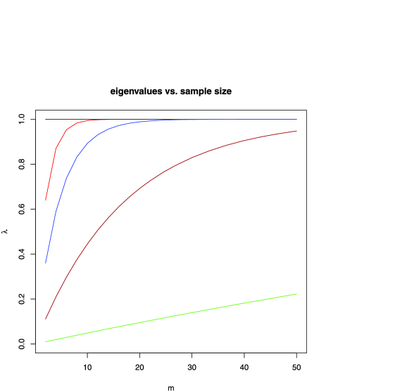
Figure 1: The behavior of the dominant eigenvalue for the MDA chain in the Bernoulli model. The graph shows how the dominant eigenvalue of the MDA chain changes with sample size, $m$, for several different values of $\rho$, in the case where half the $z_{i}$’s are 0 and the other half are 1. (Only even sample sizes are considered.) The red, blue, brown and green lines correspond to $\rho$ values of $1/10$, $1/5$, $1/3$ and $9/20$, respectively.

Now consider implementing the FS algorithm for the Bernoulli mixture. Because the mixture has only two components, the random label switching step, ${\mathbf{y}}\rightarrow{\mathbf{y}}^{\prime}$, is quite simple. Indeed, we simply flip a fair coin. If the result is heads, then we take ${\mathbf{y}}^{\prime}={\mathbf{y}}$, and if the result is tails, then we take ${\mathbf{y}}^{\prime}=\overline{{\mathbf{y}}}$, where $\overline{{\mathbf{y}}}$ denotes ${\mathbf{y}}$ with its 1’s and 2’s flipped. The Mtm of the FS chain has entries given by

$$\tilde{k}(r^{\prime},s^{\prime}|r,s)=\frac{1}{2}\sum_{{\mathbf{y}}\in{\mathsf{Y}}}\pi(r^{\prime},s^{\prime}|\overline{{\mathbf{y}}},{\mathbf{z}})\pi({\mathbf{y}}|r,s,{\mathbf{z}})+\frac{1}{2}\sum_{{\mathbf{y}}\in{\mathsf{Y}}}\pi(r^{\prime},s^{\prime}|{\mathbf{y}},{\mathbf{z}})\pi({\mathbf{y}}|r,s,{\mathbf{z}}).$$

It follows that

$$\tilde{k}=\left[\matrix{\frac{\rho^{m_{1}}(1-\rho)^{m_{0}}}{2^{m}}w_{0}(\rho)&\frac{1}{2^{m}}w_{1}(\rho)&\frac{1}{2^{m}}w_{1}(\rho)&\frac{\rho^{m_{0}}(1-\rho)^{m_{1}}}{2^{m}}w_{0}(\rho)\vspace*{2pt}\cr\rho^{m_{1}}(1-\rho)^{m_{0}}w_{1}(\rho)&\frac{w_{2}(\rho)+\rho^{m}(1-\rho)^{m}w_{0}(\rho)}{2}&\frac{w_{2}(\rho)+\rho^{m}(1-\rho)^{m}w_{0}(\rho)}{2}&\rho^{m_{0}}(1-\rho)^{m_{1}}w_{1}(\rho)\vspace*{2pt}\cr\rho^{m_{1}}(1-\rho)^{m_{0}}w_{1}(\rho)&\frac{w_{2}(\rho)+\rho^{m}(1-\rho)^{m}w_{0}(\rho)}{2}&\frac{w_{2}(\rho)+\rho^{m}(1-\rho)^{m}w_{0}(\rho)}{2}&\rho^{m_{0}}(1-\rho)^{m_{1}}w_{1}(\rho)\vspace*{2pt}\cr\frac{\rho^{m_{1}}(1-\rho)^{m_{0}}}{2^{m}}w_{0}(\rho)&\frac{1}{2^{m}}w_{1}(\rho)&\frac{1}{2^{m}}w_{1}(\rho)&\frac{\rho^{m_{0}}(1-\rho)^{m_{1}}}{2^{m}}w_{0}(\rho)}\right].$$

Note that this matrix differs from $k$ only in the middle four elements. Indeed, the $(2,2)$ and $(2,3)$ elements in $k$ have both been replaced by their average in $\tilde{k}$, and the same is true of the $(3,2)$ and $(3,3)$ elements. The matrix $\tilde{k}$ has rank at most two, so there is at most one nonzero eigenvalue to find. Using the results in the Appendix along with the eigen-analysis of $k$ performed earlier, it is easy to see that the nontrivial eigen-solution of $\tilde{k}$ is $(\tilde{v}_{1},\tilde{\lambda}_{1})=(v_{2},\lambda_{2})$. So, the effect on the spectrum of adding the random label switching step is to replace the dominant eigenvalue with 0! (Note that Theorem 1 implies that $\lambda_{2}=\tilde{\lambda}_{1}\leq\lambda_{1}$, which justifies our ordering of the eigenvalues of $k$.) Consider again the simple numerical example with the $50\dvtx 50$ split of 0’s and 1’s. In the case $m=10$, the result of adding the extra step is to replace the dominant eigenvalue, $0.99395$, by $0.19795$. When $m=20$, $0.99996$ is replaced by $0.15195$. This suggests that, in contrast to the MDA algorithm, increasing sample size does not adversely affect the FS algorithm. More evidence for this is provided in Figure 2, which is the analogue of Figure 1 for the FS algorithm. Note that the dominant eigenvalues are now substantially smaller, and no longer converge to 1 as the sample size increases. In fact, based on experimental evidence, it appears that, for a fixed value of $\rho$, $\lambda_{2}$ hits a maximum and then decreases with sample size. It is surprising that such a minor change in the MDA algorithm could result in such a huge improvement. In the next section we consider a mixture of normal densities.

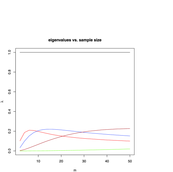
Figure 2: The behavior of the dominant eigenvalue for the FS chain in the Bernoulli model. The graph shows how the dominant eigenvalue of the FS chain changes with sample size, $m$, for several different values of $\rho$, in the case where half the $z_{i}$’s are 0 and the other half are 1. (Only even sample sizes are considered.) The red, blue, brown and green lines correspond to $\rho$ values of $1/10$, $1/5$, $1/3$ and $9/20$, respectively.

6.2 The Normal Mixture

Assume that $Z_{1},\ldots,Z_{m}$ are i.i.d. from the density

$$f(z|\mu,\tau^{2},p)=p\frac{1}{\tau_{1}}\phi\biggl{(}\frac{z-\mu_{1}}{\tau_{1}}\biggr{)}+(1-p)\frac{1}{\tau_{2}}\phi\biggl{(}\frac{z-\mu_{2}}{\tau_{2}}\biggr{)},$$

where $p\in[0,1]$, $\mu=(\mu_{1},\mu_{2})\in\mathbb{R}^{2}$, $\tau^{2}=(\tau^{2}_{1},\tau^{2}_{2})\in\mathbb{R}^{2}_{+}$, and $\phi(\cdot)$ denotes the standard normal density function. The prior for $p$ is $\operatorname{Uniform}(0,1)$, and the prior for $(\mu,\tau^{2})$ takes the form $\pi(\mu_{1},\tau^{2}_{1})\pi(\mu_{2},\tau^{2}_{2})$. As for $\pi$, we use the standard (conditionally conjugate) prior given by

$$\pi(\mu_{1},\tau^{2}_{1})=\pi(\mu_{1}|\tau^{2}_{1})\pi(\tau^{2}_{1}),$$

where $\pi(\mu_{1}|\tau^{2}_{1})=\mathrm{N}(0,\tau^{2}_{1})$ and $\pi(\tau^{2}_{1})=\operatorname{IG}(2,1/2)$ (Robert and Casella, 2004, Section 9.1). By $W\sim\operatorname{IG}(\alpha,\gamma)$, we mean that $W$ is a random variable with density function proportional to $w^{-\alpha-1}\exp\{-\gamma/w\}\cdot I_{\mathbb{R_{+}}}(w)$. In contrast with the Bernoulli example from the previous subsection, the posterior density associated with the normal mixture is quite intractable and has a complicated (and uncountable) support given by ${\mathsf{X}}=\mathbb{R}^{2}\times\mathbb{R}^{2}_{+}\times[0,1]$.

The MDA algorithm is based on the complete-data posterior density, which we denote here by $\pi(\mu,\tau^{2},p,\allowbreak{\mathbf{y}}|{\mathbf{z}})$. Again, the development in Section 5.1 implies that, given $(\mu,\tau^{2},p,{\mathbf{z}})$, the elements of ${\mathbf{y}}$ are independent multinomials and the probability that the $i$th coordinate equals 1 (which is one minus the probability that it equals 2) is given by

$$\biggl{(}p\frac{1}{\tau_{1}}\phi\biggl{(}\frac{z_{i}-\mu_{1}}{\tau_{1}}\biggr{)}\biggr{)}\Big{/}\biggl{(}p\frac{1}{\tau_{1}}\phi\biggl{(}\frac{z_{i}-\mu_{1}}{\tau_{1}}\biggr{)}+(1-p)\frac{1}{\tau_{2}}\phi\biggl{(}\frac{z_{i}-\mu_{2}}{\tau_{2}}\biggr{)}\biggr{)}.$$ (17)

We sample $\pi(\mu,\tau^{2},p|{\mathbf{y}},{\mathbf{z}})$ via sequential sampling from $\pi(p|{\mathbf{y}},{\mathbf{z}})$ and $\pi(\mu,\tau^{2}|p,{\mathbf{y}},{\mathbf{z}})$. The results in Section 5.1 show that $p|{\mathbf{y}},{\mathbf{z}}\sim\operatorname{Beta}(c_{1}+1,c_{2}+1)$. Moreover, it’s easy to show that, given $(p,{\mathbf{y}},{\mathbf{z}})$, $(\mu_{1},\tau^{2}_{1})$ and $(\mu_{2},\tau^{2}_{2})$ are independent. Routine calculations show that

$$\mu_{1}|\tau_{1}^{2},p,{\mathbf{y}},{\mathbf{z}}\sim\mathrm{N}\biggl{(}\frac{c_{1}}{c_{1}+1}\overline{z}_{1},\frac{\tau^{2}_{1}}{(c_{1}+1)}\biggr{)}$$

and

$$\tau_{1}^{2}|p,{\mathbf{y}},{\mathbf{z}}\sim\operatorname{IG}\biggl{(}\frac{c_{1}+4}{2},\frac{1}{2}\biggl{(}s_{1}^{2}+\frac{c_{1}\overline{z}_{1}^{2}}{(c_{1}+1)}+1\biggr{)}\biggr{)},$$

where $\overline{z}_{1}=\frac{1}{c_{1}}\sum_{i=1}^{m}I_{\{1\}}(y_{i})z_{i}$ and $s_{1}^{2}=\sum_{i=1}^{m}I_{\{1\}}(y_{i})\cdot(z_{i}-\overline{z}_{1})^{2}$. Of course, the distribution of $(\mu_{2},\tau^{2}_{2})$ given $(p,{\mathbf{y}},{\mathbf{z}})$ has an analogous form.

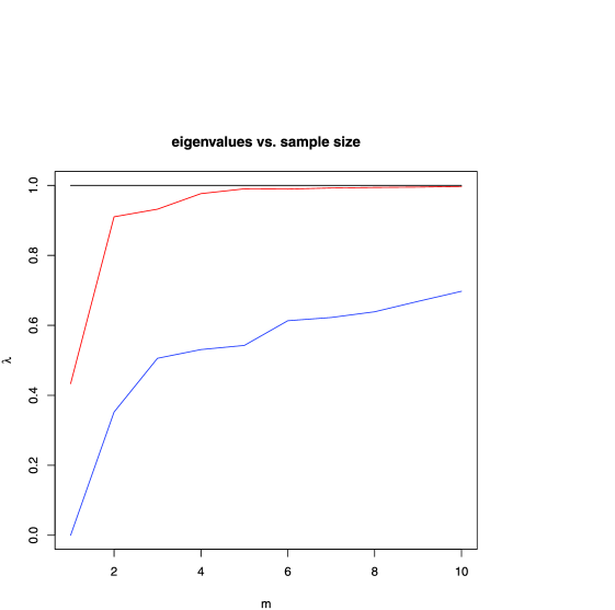
Figure 3: The behavior of the dominant eigenvalue for the MDA and FS chains in the normal model. The graph is based on the first simulated data set and shows how the dominant eigenvalue changes with sample size, $m$, for the MDA algorithm (red line) and the FS algorithm (blue line).

The results developed in Section 3 imply that the spectrum of the operator associated with the MDA chain consists of the point $\{0\}$ and the eigenvalues of the Mtm of the conjugate chain, which lives on ${\mathsf{Y}}=\{1,2\}^{m}$. Unfortunately, the Mtm of the conjugate chain is also intractable. Indeed, a generic element of this matrix has the following form:

$$\hat{k}({\mathbf{y}}^{\prime}|{\mathbf{y}})=\int_{0}^{1}\int_{\mathbb{R}^{2}_{+}}\int_{\mathbb{R}^{2}}\pi({\mathbf{y}}^{\prime}|\mu,\tau^{2},p,{\mathbf{z}})\cdot\pi(\mu,\tau^{2},p|{\mathbf{y}},{\mathbf{z}})\,d\mu\,d\tau^{2}\,dp.$$

This integral cannot be computed in closed form. In particular, $\pi({\mathbf{y}}^{\prime}|\mu,\tau^{2},p,{\mathbf{z}})$ is the product of $m$ probabilities of the form (17), and the sums in the denominators of these probabilities render the integral intractable. However, note that $\hat{k}({\mathbf{y}}^{\prime}|{\mathbf{y}})$ can be interpreted as the expected value of $\pi({\mathbf{y}}^{\prime}|\mu,\tau^{2},p,{\mathbf{z}})$ with respect to the density $\pi(\mu,\tau^{2},p|{\mathbf{y}},{\mathbf{z}})$. Of course, for fixed ${\mathbf{z}}$, we know how to draw from $\pi(\mu,\tau^{2},p|{\mathbf{y}},{\mathbf{z}})$, and we have $\pi({\mathbf{y}}^{\prime}|\mu,\tau^{2},p,{\mathbf{z}})$ in closed form. We therefore have the ability to estimate $\hat{k}({\mathbf{y}}^{\prime}|{\mathbf{y}})$ using classical Monte Carlo. Once we have an estimate of the entire $2^{m}\times 2^{m}$ Mtm, we can calculate its eigenvalues.

The same idea can be used to approximate the eigenvalues of the FS chain. The results in Section 4 show that we can express the FS algorithm as a DA algorithm with respect to an alternative complete-data posterior density, which we write as $\pi^{*}(\mu,\tau^{2},p,{\mathbf{y}}|{\mathbf{z}})$. The eigenvalues of the operator defined by the FS chain are the same as those of the Mtm in which the probability of the transition ${\mathbf{y}}\rightarrow{\mathbf{y}}^{\prime}$ is given by

$$\int_{0}^{1}\int_{\mathbb{R}^{2}_{+}}\int_{\mathbb{R}^{2}}\pi^{*}({\mathbf{y}}^{\prime}|\mu,\tau^{2},p,{\mathbf{z}})\cdot\pi^{*}(\mu,\tau^{2},p|{\mathbf{y}},{\mathbf{z}})\,d\mu\,d\tau^{2}\,dp.$$

It is straightforward to simulate from $\pi^{*}(\mu,\tau^{2},p|{\mathbf{y}},{\mathbf{z}})$, and $\pi^{*}({\mathbf{y}}^{\prime}|\mu,\tau^{2},p,{\mathbf{z}})$ is available in closed form.

To use our classical Monte Carlo idea to estimate the spectra associated with the MDA and FS chains, we must specify the data, ${\mathbf{z}}$. Furthermore, the Bernoulli example in the previous subsection showed that the convergence rates of the two algorithms can depend heavily on the sample size, $m$. Thus, we would like to explore how an increasing sample size affects the convergence rates of the MDA and FS chains in the current context. To generate data, we simulated a random sample of size 10 from a $50\dvtx 50$ mixture of a $\mathrm{N}(0,0.55^{2})$ and a $\mathrm{N}(3,0.55^{2})$, and this resulted in the following observations:

$${\mathbf{z}}=(z_{1},\ldots,z_{10})=(0.2519,2.529,-0.2930,2.799,3.397,0.5596,2.810,2.541,2.487,-0.1937).$$

We considered 10 different data sets ranging in size from $m=1$ to $m=10$. The first data set contained the single point $z_{1}=0.25192$, the second contained the first two observations $(z_{1},z_{2})=(0.25192,2.5287)$, the third contained $(z_{1},z_{2},z_{3})=(0.25192,2.5287,-0.29303)$, and so on up to the tenth data set, which contained all ten observations. For each of these 10 data sets, we used the classical Monte Carlo technique described above to estimate the Mtm for both the MDA and FS algorithms. In particular, for each row of the Mtm we used a single Monte Carlo sample of size 200,000 [from $\pi(\mu,\tau^{2},p|{\mathbf{y}},{\mathbf{z}})$ for DA, and from $\pi^{*}(\mu,\tau^{2},p|{\mathbf{y}},{\mathbf{z}})$ for FS] to estimate each of the entries in that row. We then calculated the eigenvalues of the estimated Mtms and recorded the largest one. The results are shown in Figure 3, which has some interesting features. Note that the dominant eigenvalues of the MDA chain are much closer to 1 than the corresponding dominant eigenvalues of the FS chain. Even at $m=5$, the dominant eigenvalue of the MDA chain is already above 0.99. As in the previous example, the convergence rate of the MDA chain deteriorates as $m$ increases. It is not clear whether the FS chain slows down as $m$ increases. It may be the case that the FS eigenvalue would eventually level off, or perhaps the FS chain would eventually begin to speed up, as in the Bernoulli example. Note that, as proven in Section 5.2, when $m=1$, the FS eigenvalue is 0. (To ascertain the accuracy of our estimates, we repeated the entire classical Monte Carlo simulation 6 times, with different random number seeds, and based on this, we believe that our eigenvalue estimates are correct up to three decimal places.)

In the case where all 10 observations are considered, the dimension of the Mtms is $1024\times 1024$, and each element must be estimated by classical Monte Carlo. Thus, while it would be very interesting to consider larger sample sizes (beyond 10), and even mixtures with more than 2 components, the matrices become quite unwieldy.

We simulated a second set of 10 observations from the same $50\dvtx 50$ mixture and repeated the entire process for the purpose of validation. The second simulation resulted in the following data:

$${\mathbf{z}}=(z_{1},\ldots,z_{10})=(0.6699,3.408,0.1093,3.289,-0.1407,3.525,2.454,0.2716,-0.7443,3.570).$$

Figure 4 is the analogue of Figure 3 for the second simulation. The results are nearly identical to those from the first simulation.

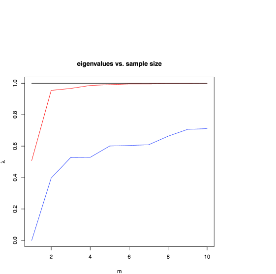
Figure 4: The behavior of the dominant eigenvalue for the MDA and FS chains in the normal model. The graph is based on the second simulated data set and shows how the dominant eigenvalue changes with sample size, $m$, for the MDA algorithm (red line) and the FS algorithm (blue line).

Appendix

Consider a Mtm of the form

$$M=\left[\matrix{a&b&b&c\cr d&e&f&\frac{cd}{a}\vspace*{2pt}\cr d&f&e&\frac{cd}{a}\cr a&b&b&c}\right],$$

and assume that all of the elements are strictly positive, so the corresponding Markov chain is irreducible and aperiodic. Note that both of the Mtms studied in Section 6.1 have this form. Routine manipulation shows that $M$ is reversible with respect to $(\pi_{1},\pi_{2},\pi_{3},\pi_{4})^{T}$ where $\pi_{1}=ad/(ad+2ab+cd)$, $\pi_{2}=b\pi_{1}/d$, $\pi_{3}=\pi_{2}$ and $\pi_{4}=c\pi_{1}/a$. In the remainder of this section we perform an eigen-analysis of the matrix $M$.

Of course, since $M$ is a Mtm, it satisfies $kv_{0}=\lambda_{0}v_{0}$ where $v_{0}=\mathbf{1}$ and $\lambda_{0}=1$. Furthermore, since the first and fourth rows are equal, there is at least one eigenvalue equal to zero. Indeed, $Mv_{3}=0$, where $v_{3}=(c,0,0,-a)^{T}$. We now identify the other two eigen-solutions of $M$. Let $v_{1}=(0,1,-1,0)^{T}$ and note that

$$Mv_{1}=(e-f)v_{1},$$

so $\lambda_{1}=(e-f)$ is an eigenvalue. If $e=f$, then the middle two rows of $M$ are equal and the rank of $M$ is at most 2. (Note that $\lambda_{1}$ could be negative, implying that the operator defined by $M$ is not always positive.)

Now, let $v_{2}=(\alpha,1,1,\alpha)^{T}$, where $\alpha$ is a constant to be determined, and note that

$$Mv_{2}=\left[\matrix{\alpha a+2b+\alpha c\cr\alpha d+e+f+\alpha\frac{cd}{a}\vspace*{2pt}\cr\alpha d+e+f+\alpha\frac{cd}{a}\cr\alpha a+2b+\alpha c}\right].$$

If $v_{2}$ is an eigenvector with corresponding eigenvalue $\lambda_{2}$, then the first element of $Mv_{2}$ must equal $\alpha\lambda_{2}$, that is,

$$\alpha a+2b+\alpha c=\alpha\lambda_{2}.$$

Now, using the fact that $2b=1-a-c$, we have

$$(\alpha-1)(a+c)+1=\alpha\lambda_{2},$$

and it follows that

$$\lambda_{2}=\frac{(\alpha-1)(a+c)+1}{\alpha}.$$ (1)

Again, if $v_{2}$ is an eigenvector with corresponding eigenvalue $\lambda_{2}$, then the second element of $Mv_{2}$ must equal $\lambda_{2}$, or

$$\lambda_{2}=\alpha d+e+f+\alpha\frac{cd}{a}.$$

Now, using the fact that $e=1-d-f-\frac{cd}{a}$, we have

$$\lambda_{2}=\frac{d}{a}(\alpha-1)(a+c)+1.$$

Setting our two expressions for $\lambda_{2}$ equal yields

$$\alpha d(\alpha-1)(a+c)+a\alpha=a(\alpha-1)(a+c)+a.$$

This quadratic in $\alpha$ has two roots: $\alpha=1$ and

$$\alpha=\frac{a(a+c-1)}{d(a+c)}.$$

The second solution is negative and corresponds to a nontrivial eigenvector. The corresponding eigenvalue is

$$\lambda_{2}=\frac{1}{a}(a+c)(a-d).$$

If $a=d$, then the sum of the middle two rows of $M$ is equal to twice the first row.

References

- Asmussen and Glynn (2011) {barticle}[auto:STB—2011/08/02—11:14:52] \bauthor\bsnmAsmussen, \bfnmS.\binitsS. and \bauthor\bsnmGlynn, \bfnmP.\binitsP. (\byear2011). \btitleA new proof of convergence of MCMC via the ergodic theorem. \bjournalStatist. Probab. Lett. \bvolume81 \bpages1482–1485. \bptokimsref \endbibitem
- Buja (1990) {barticle}[mr] \bauthor\bsnmBuja, \bfnmAndreas\binitsA. (\byear1990). \btitleRemarks on functional canonical variates, alternating least squares methods and ACE. \bjournalAnn. Statist. \bvolume18 \bpages1032–1069. \biddoi=10.1214/aos/1176347739, issn=0090-5364, mr=1062698 \bptokimsref \endbibitem
- Celeux, Hurn and Robert (2000) {barticle}[mr] \bauthor\bsnmCeleux, \bfnmGilles\binitsG., \bauthor\bsnmHurn, \bfnmMerrilee\binitsM. and \bauthor\bsnmRobert, \bfnmChristian P.\binitsC. P. (\byear2000). \btitleComputational and inferential difficulties with mixture posterior distributions. \bjournalJ. Amer. Statist. Assoc. \bvolume95 \bpages957–970. \bidissn=0162-1459, mr=1804450 \bptokimsref \endbibitem