Bigraphical models for protein and membrane interactions

Abstract

We present a bigraphical framework suited for modeling biological systems both at protein level and at membrane level. We characterize formally bigraphs corresponding to biologically meaningful systems, and bigraphic rewriting rules representing biologically admissible interactions. At the protein level, these bigraphic reactive systems correspond exactly to systems of $\kappa$-calculus. Membrane-level interactions are represented by just two general rules, whose application can be triggered by protein-level interactions in a well-defined and precise way.

This framework can be used to compare and merge models at different abstraction levels; in particular, higher-level (e.g. mobility) activities can be given a formal biological justification in terms of low-level (i.e., protein) interactions. As examples, we formalize in our framework the vesiculation and the phagocytosis processes.

1 Introduction

Cardelli in [8] has convincingly argued that the various biochemical toolkits identified by biologists can be described as a hierarchy of abstract machines, each of which can be modelled using methods and techniques from concurrency theory. These machines are highly interdependent: “to understand the functioning of a cell, one must understand also how the various machines interact” [8]. Like other complex situations, it seems unlikely to find a single notation covering all aspects of a whole organism. In fact, we are in presence of a tower of models [19], each focusing on specific aspects of the biological system, at different levels of abstractions. Higher-level models must be represented, or realised, at a lower level, and where possible this representation must be proved sound; in addition, we need to combine different models at the same level. To this end, we need a general metamodel, that is, a framework, where these models (possibly at different abstraction levels) can be encoded, and their interactions can be formally described.

In this paper, we substantiate Milner’s idea that bigraphs can be successfully used as a framework for systems biology. More precisely, we define a class of biological bigraphs, and biological bigraphical reactive systems (BioRS), for dealing with both protein-level and membrane-level interactions.

An important design choice is that this framework has to be biologically sound, i.e., it must admit only systems and reactions which are biologically meaningful, especially at lower level machines (i.e. protein). In this way, encoding a given model, for any abstract machine, as a BioRS provides automatically a formal, biologically sound justification for the model (or “implementation”) in terms of protein reactions and explains how its membrane-level interactions are realised by protein machinery.

In order to formalize this “biological soundness”, we need a formal protein model to compare to our framework. We choose Danos and Laneve’s $\kappa$-calculus, one of the most accepted formal model of protein systems. By suitable sorting conditions, we define a bigraphical framework which allows all and only protein configurations and interactions of the $\kappa$-calculus. It is important to notice, however, that our methodology is general, and can be applied to other formal protein models.

On the other hand, membrane nesting reconfiguration can be performed by just only two general rules, corresponding to the natural phenomena of “pinch” and “fuse” [10]. For encoding a given membrane model one has just to refine this general schema by specifying when these reactions are triggered, that is, when the right proteins are in place. Indeed, as observed by biologists (see [1] and [2, Ch. 15]), membrane interactions present always a “preparation phase”, where membrane proteins (receptors and ligands) interact, followed by the actual “membrane reconfiguration” phase. The “pinch” and “fuse” rules model the latter phase, whilst the preparation phase depends on the specific proteins involved and hence left to the encoding of the specific model under examination.

Another important consequence of encoding a model in our framework is that any “too abstract”, or non-realistic, aspect of the model is readily identified, because its formalization turns out to be problematic, or even impossible. In this case, one has to change the model, or the encoding, in order to be biologically sound. As a result, the bigraphical encoding of a given system may exhibit unexpected features, not present (or unpredicted) in the original model. Far from being a problem, this allows to foresee emerging properties, such as behaviours due to interactions of different abstraction levels, and which cannot be observed within a single machine model due to its intrinsic abstractions.

A further motivation for our framework comes from the many general results provided by bigraphs. We mention here only the construction of compositional bisimilarities [18], allowing to prove that two systems are observational equivalent, that is, they can be exchanged in any organism without that the overall behaviour will change. Also for this application it is important to restrict the bigraphs allowed by the framework to only those biologically meaningful.

We summarise briefly our approach. In Section 3 we first define protein link graphs and corresponding reactive systems, which correspond precisely to protein solutions and protein transition systems of the $\kappa$-calculus (recalled in Section 2.2). In Section 4 we extend this approach to deal with compartments, introducing biobigraphs. Membranes are represented by two new nodes, which play no role at the protein level, but which can contain other systems. Appropriate sorting conditions will enforce biological properties such as bitonality and orientation of membranes. Two applications of this frameworks are given in Section 5: a formal description of vesicle formation process, and a formalization of the Fc receptor-mediated phagocytosis. In both cases, the framework obliges to provide a formal justification of (membrane mobility) reactions in terms of protein-level interactions. Conclusions are in Section 6.

2 Preliminaries

2.1 Bigraphical reactive systems

In this section we recall the bigraphical framework [18], extending the variant of [5] with typed names.

Bigraphs A bigraph represents an open system, so it has an inner and an outer interface to “interact” with subsystems and the surrounding environment. The numbers in the interfaces describe the roots in the outer interface (that is, the various locations where the nodes live) and the sites in the inner interface (that is, the grey holes where other bigraphs can be inserted). On the other hand, the names in the interfaces describes the open links, that is end points where links from the outside world can be pasted, creating new links among nodes. An example of a bigraph is shown in Fig. 1.

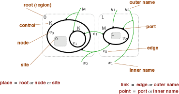
Figure 1: Example of a bigraph and its structure (picture from Milner’s slide).

A signature is a quadruple $\langle\mathcal{K},ar,\mathcal{T},\mathcal{E}\rangle$ where $\mathcal{K}$ is a set of node controls with an arity function $ar\colon\mathcal{K}\to\mathbb{N}$, $\mathcal{T}$ is a poset of types with ordering $\sqsubseteq$, and $\mathcal{E}\subseteq\mathcal{T}$ denotes the edge types.

Definition 2.1 (Interfaces and Bigraphs).

An interface is a pair $\langle n,X\rangle$, where $n$ is a finite ordinal (called width) and $X$ is a set of typed names $x{:\,}\mathsf{t}$, where $\mathsf{t}\in\mathcal{T}$.

A bigraph $G$ is composed by a place graph $G^{P}$, describing the nesting of nodes, and a link graph $G^{L}$, describing the (hyper-)links among nodes.

$$G^{P} =(V,ctrl,prnt)\colon m\to n$$ (Place graph)

$$G^{L} =(V,E,ctrl,edge,link)\colon X\to Y$$ (Link graph)

$$G =(G^{P},G^{L})=(V,E,ctrl,edge,prnt,link)\colon\langle m,X\rangle\to\langle n,Y\rangle$$ (Bigraph)

where $V,E$ are the sets of nodes and edges respectively, $ctrl\colon V\to\mathcal{K}$ is the control map, which assigns a control to each node, $edge\colon E\to\mathcal{E}(\subseteq\mathcal{T})$ is the edge typing which assigns a type to each edge, $prnt\colon m\uplus V\to V\uplus n$ is the (acyclic) parent map, the disjoint sum $Prt=\sum_{v\in V}ar(ctrl(v))$ is the set of ports (associated to all nodes), and $link\colon X\uplus Prt\to E\uplus Y$ is the (type consistent) link map, i.e., for all $x{:\,}\mathsf{t}\in X$, if $link(x{:\,}\mathsf{t})=l{:}\mathsf{t}^{\prime}$ then $\mathsf{t}\sqsubseteq\mathsf{t}^{\prime}$.

In the following, we say place to mean a node, a root or a site, and we call the elements in the domain of the link map points, while the ones in the codomain links. An idle name is not a target of any point. We denote by $(v,i)$ the $i$th port of the node $v$. Two nodes are peer if two of their port (one per node) have the same target link. Often, we say control to mean a node with associate that control, and we write $x\in X$ in place of $x{:\,}\mathsf{t}\in X$ when the type of the name it is clear from the context.

Definition 2.2 (Bigraph category).

Given a signature $\langle\mathcal{K},ar,\mathcal{T},\mathcal{E}\rangle$, the category of (link typed) bigraphs ${\textsc{Big}}(\mathcal{K},\mathcal{T},\mathcal{E})$ has interfaces as objects and bigraphs as morphisms.

Given two bigraphs $G\colon\langle m,X\rangle\to\langle n,Y\rangle$, $H\colon\langle n,Y\rangle\to\langle k,Z\rangle$, the composition $H\circ G\colon\langle m,X\rangle\to\langle k,Z\rangle$ is defined by composing their place and link graphs:

Place:

$H^{P}\circ G^{P}=(V,ctrl,(id_{V_{G}}\cup prnt_{H})\circ(prnt_{G}\cup id_{V_{H}}))\colon m\to k$;

Link:

$H^{L}\circ G^{L}=(V,E,ctrl,edge,(id_{E_{G}}\cup link_{H})\circ(link_{G}\cup id_{P_{H}}))\colon X\to Z$,

where $V=V_{G}\cup V_{H}$, $E=E_{G}\cup E_{H}$ (supposing $V_{G}\cap V_{H}=E_{G}\cap E_{H}=\emptyset$ otherwise a renaming is applied), $ctrl=ctrl_{G}\cup ctrl_{H}$ and $edge=edge_{G}\cup edge_{H}$.

Plg and Lnk will denote the categories of place and link graphs, respectively.

An example of splitting of a bigraph in its components is shown in Figure 2.

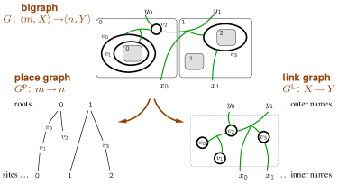
Figure 2: Splitting of a bigraph (picture from [18]), where $m=2$, $n=1$, $X=\{x_{0},x_{1}\}$, $Y=\{y_{0},y_{1}\}$.

Intuitively, composition is performed in two steps. First, the place graph are composed by putting the roots of the “lower” bigraph inside the sites (i.e., holes) of the “upper” one, respecting the order given by the ordinal in the interface; then, the links are connected by sticking together the end parts of connections in the two link graphs, labelled with the same typed name in the common interface.

An important operation on bigraphs is the tensor product. Intuitively, the tensor product of $G:\langle m,X\rangle\to\langle n,Y\rangle$ and $H:\langle m^{\prime},X^{\prime}\rangle\to\langle n^{\prime},Y^{\prime}\rangle$, defined when $X\cap X^{\prime}=Y\cap Y^{\prime}=\emptyset$, is the bigraph $G\otimes H:\langle m+m^{\prime},X\uplus X^{\prime}\rangle\to\langle n+n^{\prime},Y\uplus Y^{\prime}\rangle$ and is obtained by putting “side by side” $G$ and $H$. Two useful variant of tensor product can be defined using tensor and composition: the parallel product $\parallel$, which merges shared names between two bigraphs, and the prime product $\mid$, that moreover merges all roots in a single one. We refer to [18] for formal definitions.

Bigraphical reactive systems (BRSs) are reactive systems in the sense of [17], built over the category ${\textsc{Big}}(\mathcal{K},\mathcal{T},\mathcal{E})$ [18, 5]. A BRS consists of a set of bigraphical rewriting rules, together with a definition of the evaluation contexts (i.e., bigraphs with holes) where rules redexes can be found in order to be rewritten. Such contexts are defined as a sub-category $\mathcal{A}$ of active context inside ${\textsc{Big}}(\mathcal{K},\mathcal{T},\mathcal{E})$.

Definition 2.3 (Activity).

Each control of a signature is either active or passive or atomic. An atomic control cannot contain any node (hence it is a leaf on the place graph). A location (i.e., an element in the domain of $prnt$) is active if all its ancestors have active controls (roots are always active); otherwise it is passive. A context is active if all its holes are active locations.

It is easy to check that active contexts form a compositional reflective sub-category of bigraphs, which we denote by $\mathcal{A}$, the category of active contexts.

Definition 2.4 (BRS).

A bigraphical reactive system $\mathcal{D}(\mathcal{K},\mathcal{T},\mathcal{E},\mathcal{R})$ is formed by ${\textsc{Big}}(\mathcal{K},\mathcal{T},\mathcal{E})$ equipped with the subcategory Act of active contexts, and a set $\mathcal{R}$ of (parametric) reaction rules, that is pairs $L,R:\langle m,X\rangle\to\langle n,Y\rangle$ (usually written as $L\rightarrowtriangle R$). The reaction relation $\rightarrowtriangle$ defined by a BRS is the relation between ground bigraphs given by the following rule:

$$\frac{C\in{\textsc{Act}}\qquad L\rightarrowtriangle R\in\mathcal{R}\qquad d\text{ ground}\qquad G=C\circ L\circ d\qquad H=C\circ R\circ d}{G\rightarrowtriangle H}$$

Clearly, these definitions can be applied to place and link graphs too. Active contexts for place graphs are as for bigraphs and the rules can have only holes; instead for link graphs, all contexts are active.

Sortings Usually, bigraphs defined over a given signature are “too many”. A systematic way for ruling out unwanted bigraphs is by means of a sorting [4], that is, a functor $F\colon{\textsc{S}}\to{\textsc{Big}}$, faithful and surjective on objects, defined on a category S where unwanted morphisms from Big are deleted. A sorting can be conveniently defined by means of a suitable logical condition specifying the class of morphisms we want to restrict to [4]. To ease readability, in the paper we will present these conditions in a semi-formal logical language; a formal description of all these conditions can be given as BiLog formulas [12] (see Appendix B) . Notice that also the name typing introduced in Definition 2.1 can be expressed by means of a sorting.

2.2 The $\kappa$-calculus

Here we recall Danos and Laneve’s $\kappa$-calculus [14], a calculus for protein interactions, which will be our reference protein-level model in Section 3.

Let $\mathcal{P}$ be a finite set of proteins and $\mathcal{N}$ an enumerable set of edge names. Let $s\colon\mathcal{P}\to\mathbb{N}$ be a signature, that assigns to every protein the number of its domain sites. A $\kappa$-interface is a map from $\mathbb{N}$ to $\mathcal{N}\uplus\{h,v\}$ (ranged over $\rho$, $\sigma$, $\ldots$). Given an interface $\rho$ and a protein name $A\in\mathcal{P}$, a site $(A,i)$ is visible if $\rho(i)=v$, hidden if $\rho(i)=h$, and tied if $\rho(i)\in\mathcal{N}$. A site is free if it is visible or hidden. In the following, we will write $\rho=1+\bar{2}+3^{x}$ to mean $\rho(1)=v$, $\rho(2)=h$, and $\rho(3)=x$. The syntax of $\kappa$-solutions is the following:

$$S,T::=\mathbf{0}\mid A(\rho)\mid S\mathop{,}T\mid(x)(S)$$

up-to $\alpha$-equivalence and the least structural equivalence ($\equiv$), satisfying the abelian monoid on composition and the scope extension and extrusion laws. The sets of free edge names $fn(\rho)$ and $fn(S)$, on interfaces and solutions, are defined as usual.

Definition 2.5.

The set of connected $\kappa$-solutions is defined inductively as:

$$\frac{\displaystyle}{\displaystyle A(\rho)}\qquad\frac{\displaystyle S}{\displaystyle(x)S}\qquad\frac{\displaystyle S\quad T\quad fn(S)\cap fn(T)\neq\emptyset}{\displaystyle S\mathop{,}T}\qquad\frac{\displaystyle S\quad S\equiv T}{\displaystyle T}$$

Definition 2.6.

A $\kappa$-solution $S$ is (strong) graph-like if free names occur at most (exactly) two times in $S$, and binders tie either 0 or 2 occurrences.

A complex is a closed, graph-like, and connected solution.

Biochemical reactions are either complexations (i.e. where low energy bonds are formed on two complementary sites) or decomplexations, possibly co-occurring with (de)activation of sites. Causality does not allow simultaneous complexations and decomplexations on the same site: this biological constraint is assured in the $\kappa$-calculus by the notion of (anti-)monotonicity, which forces reactions not to decrease (increase) the level of connection of a solution (see [14] for details).

Definition 2.7 (Growing relation).

Let $\tilde{x}$ be a set of fresh names.

A growing relation $\rhd$ over $\kappa$-interfaces is defined inductively as follows:

$$\frac{\displaystyle}{\displaystyle\tilde{x}\vdash\bar{i}\rhd i}\quad\;\frac{\displaystyle}{\displaystyle\tilde{x}\vdash i\rhd\bar{i}}\quad\;\frac{\displaystyle x\in\tilde{x}}{\displaystyle\tilde{x}\vdash i\rhd i^{x}}\quad\;\frac{\displaystyle\tilde{x}\cap fn(\rho)=\emptyset}{\displaystyle\tilde{x}\vdash\rho\rhd\rho}\quad\;\frac{\displaystyle\tilde{x}\vdash\rho\rhd\sigma\quad\tilde{x}\vdash\rho^{\prime}\rhd\sigma^{\prime}}{\displaystyle\tilde{x}\vdash\rho+\rho^{\prime}\rhd\sigma+\sigma^{\prime}}$$

A growing relation $\rhd$ over $\kappa$-solutions is defined inductively as follows:

$$\frac{\displaystyle}{\displaystyle\tilde{x}\vdash\mathbf{0}\rhd\mathbf{0}}\qquad\frac{\displaystyle\tilde{x}\vdash S\rhd T\quad\tilde{x}\vdash\rho\rhd\sigma}{\displaystyle\tilde{x}\vdash S\mathop{,}A(\rho)\rhd T\mathop{,}A(\sigma)}\qquad\frac{\displaystyle\tilde{x}\vdash S\rhd T\quad fn(\sigma)\subseteq\tilde{x}}{\displaystyle\tilde{x}\vdash S\rhd T\mathop{,}A(\sigma)}$$

Definition 2.8 (Monotone reactions).

Let $L,R$ be two $\kappa$-solutions. $L\rightarrow(\tilde{x})R$ is a monotone reaction if $\tilde{x}\vdash L\rhd R$, $L$ and $(\tilde{x})R$ are graph-like and $R$ is connected. $L\rightarrow(\tilde{x})R$ is an antimonotone reaction if $R\rightarrow(\tilde{x})L$ is monotone.

Finally, we are able to characterize a protein transition system:

Definition 2.9 (Protein transition systems).

Given a set $\mathcal{R}_{\kappa}$ of monotone and antimonotone reactions, we define a protein transition system (PTS) as a pair $\langle\mathcal{S},\leadsto\rangle$, such that $\mathcal{S}$ is a set of $\kappa$-solutions, and $\leadsto$ is the least binary relation over $\mathcal{S}$ such that $\mathcal{R}_{\kappa}\subseteq{\leadsto}$, closed w.r.t. $\equiv$, composition and name restriction.

3 Protein link graphs

In this section we introduce a general graphical formalism for modelling biological protein interactions. Proteins are represented as atomic nodes where links stand for chemical bonds. In such a model locations are not needed, hence we do not make use of the full bigraphical framework and link graphs are enough.

A protein changes its behaviour depending on its folding structure which determines its current interacting interface (the set of its domain sites). This structure could change after a complexation reaction. To describe the interface of each protein we use four linking types, $\mathsf{v}$ (visible), $\mathsf{h}$ (hidden), $\mathsf{b}$ (bond) and $\mathsf{f}$ (free), indicating the status of the corresponding protein site which they are connected to.

Definition 3.1 (Protein signature).

Let $\mathcal{P}$ be a set of protein controls, a protein signature $\langle\mathcal{P},ar\rangle$ is defined as $\langle\mathcal{P},ar,\mathcal{T}_{p},\mathcal{E}_{p}\rangle$, where $\mathcal{T}_{p}=\{\mathsf{h},\mathsf{v},\mathsf{b},\mathsf{f}\}$ with $\sqsubseteq_{p}=id_{\mathcal{T}_{p}}\cup\{(\mathsf{f},t):t\in\mathcal{T}_{p}\}$, and $\mathcal{E}=\{\mathsf{h},\mathsf{v},\mathsf{b}\}$.

Figure 3: An example of a wrong composition.

We say that a site is visible, hidden, bond or free if it is connected to an link of type $\mathsf{v}$, $\mathsf{h}$, $\mathsf{b}$ or $\mathsf{f}$, respectively. In principle, hyperlinks can connect more than two ports, yielding biological meaningless link graphs because a bond involves at most two sites. Clearly, we want this condition to be preserved under composition (it is always preserved by tensor). Actually, two good protein solutions could be composed yielding an incorrect solution, as in the Figure 3.

Well-formed link graphs can be defined as follows:

Definition 3.2 (Protein solution).

A protein solution $S\colon X\to Y$ is a link graph over a protein signature $\mathcal{P}$, such that every link has at most two peers, and every link of type $\mathsf{v}$ or $\mathsf{h}$ has exactly one peer:

$$\forall l:t.\;t\in\{\mathsf{b},\mathsf{f}\}\Rightarrow|link^{-1}(l:t)|\in\{1,2\}\quad\text{and}\quad\forall l:t.\;t\in\{\mathsf{h},\mathsf{v}\}\Rightarrow|link^{-1}(l:t)|=1$$ (ProtSol)

Definition 3.3 (Protein link graphs).

The category of protein link graphs Lgp is the category of link graphs sorted on the predicate ProtSol.

Let us now consider possible reaction rules on link graphs. As for $\kappa$-calculus, reactions allow complexations only between two visible sites, hence tied sites must be freed before being involved in any protein interaction. Using the same approach of [14], protein reactions can either increase or decrease the level of connection of protein complexes; they can introduce new nodes (protein synthesis) or remove nodes (protein degradation). Formally, we define a growing relation:

Definition 3.4 (Growing relation).

The growing relation $\rhd$ over pairs $(\omega,S)$ of wirings $\omega\colon Z\to Y$ and discrete solutions $S\colon X\to Z$ is defined inductively as:

$${\displaystyle\frac{}{id_{\emptyset},id_{\emptyset}\rhd id_{\emptyset},id_{\emptyset}}}\;\textsf{(empty)}\qquad\qquad{\displaystyle\frac{\omega,S\rhd\omega^{\prime},S^{\prime}}{\omega\otimes\mu,S\otimes T\rhd\omega^{\prime}\otimes\mu,S^{\prime}\otimes T}}\;\textsf{(tens)}$$

$${\displaystyle\frac{}{/z{:\,}\mathsf{v}\otimes\omega,S\rhd/z{:\,}\mathsf{h}\otimes\omega,S}}\;\textsf{(hide)}\qquad\quad{\displaystyle\frac{}{/z{:\,}\mathsf{h}\otimes\omega,S\rhd/z{:\,}\mathsf{v}\otimes\omega,S}}\;\textsf{(reveal)}$$

$${\displaystyle\frac{}{/z_{1}{:\,}\mathsf{v}\otimes/z_{2}{:\,}\mathsf{v}\otimes\omega,S\rhd(/z{:\,}\mathsf{h}\circ z/\{z_{1},z_{2}\})\otimes\omega,S}}\;\textsf{(tie)}$$

$${\displaystyle\frac{T\colon\emptyset\to\{\vec{w}\}\uplus W\qquad\mu\colon W\to\emptyset}{/\vec{z}{:\,}\mathsf{v}\otimes\omega,S\rhd(/\vec{z}{:\,}\mathsf{h}\circ(\vec{z}/\vec{w}\otimes id_{\vec{z}}))\otimes\omega\otimes\mu,S\otimes T}}\;\textsf{(synth)}$$

The growing relation can be lifted to morphisms of Lgp: $G\rhd H$ iff $\omega,G^{\prime}\rhd\mu,H^{\prime}$, where $\omega\circ G^{\prime}$, $\mu\circ H^{\prime}$ are the discrete decompositions of $G$ and $H$, respectively.

Let $G\rhd H$, according to (hide) and (reveal) $H$ can toggle free sites in $G$ from visible to hidden and vice versa, whereas (tie) allows $H$ to bind only pairs of sites that are visible in $G$. The (synth) axiom adds new proteins in the solution $H$ (possibly connected to proteins already in $G$) if their ports are all linked to edges in $H$.

Note that the discrete decomposition of a protein link graph induces a separation among protein interfaces and protein nodes. An example is given in Fig. 4.

Figure 4: An example of a growing solution: $\omega,S\rhd\mu,T$.

Now we can introduce the notion of protein reactive systems, where rewriting rules respect causality. This is guaranteed by requiring rules to either grow or shrink solutions, representing complexations and decomplexations respectively.

Definition 3.5 (Protein reactive systems).

A rule $(l,r)$ on protein link graphs is monotone if $l\rhd r$ and $r$ is connected; $(r,l)$ instead is antimonotone.

A protein reaction system (PRS) is a reactive system over Lgp, whose all reaction rules are monotone or antimonotone.

We establish now a formal correspondence between protein reactive systems and protein transition systems. We use the set of $\kappa$-protein names $\mathcal{P}$ as the set of protein controls in Lgp, using the corresponding $\kappa$-arity function $s\colon\mathcal{P}\to\mathbb{N}$.

Now, given a set $X$ of typed names, the encoding function $\llparenthesis\,\cdot\,\rrparenthesis_{X}$ mapping $\kappa$-solutions into Lgp is

$$\begin{aligned} \llparenthesis\,\mathbf{0}\,\rrparenthesis_{X}&=X&\llparenthesis\,(x)(S)\,\rrparenthesis_{X}&=/y{:\,}\mathsf{b}\circ\llparenthesis\,S\{y:\mathsf{b}/x:\mathsf{t}\}\,\rrparenthesis_{X\uplus\{y:b\}}\quad\text{where }t\in\{\mathsf{f},\mathsf{b}\}\\ \llparenthesis\,S\mathop{,}T\,\rrparenthesis_{X}&=\llparenthesis\,S\,\rrparenthesis_{X}\parallel\llparenthesis\,T\,\rrparenthesis_{X}&\llparenthesis\,A(\rho)\,\rrparenthesis_{X}&=X\parallel((\textstyle\bigparallel_{i=1}^{s(A)}\llparenthesis\,\rho(i)\,\rrparenthesis^{z_{i}}_{X})\circ A_{z_{1}:\mathsf{f}\dots z_{s(A)}:\mathsf{f}})\end{aligned}$$

$$\text{where}\quad\llparenthesis\,h\,\rrparenthesis_{X}^{z}=/z{:\,}\mathsf{h}\qquad\llparenthesis\,v\,\rrparenthesis_{X}^{z}=/z{:\,}\mathsf{v}\qquad\llparenthesis\,x\,\rrparenthesis_{X}^{z}=x:\mathsf{b}/z:\mathsf{f}\text{ (if $x\in X$)}$$

Note that $\llparenthesis\,S\,\rrparenthesis_{X}$ is defined only when $fn(S)\subseteq X$. Fig. 5 shows an example.

Figure 5: Encoding a $\kappa$-solution in a protein link graph.

We can prove the following correspondence results.

Proposition 3.1 (Syntax).

For any set of names $X$, $S\equiv T$ iff $\llparenthesis\,S\,\rrparenthesis_{X}=\llparenthesis\,T\,\rrparenthesis_{X}$.

Moreover, for all $X$, the map $\llparenthesis\,\cdot\,\rrparenthesis_{X}$ is surjective over the homset ${\textsc{Lgp}}(\emptyset,X)$.

Definition 3.6 ($\kappa$-PRS).

A $\kappa$-PRS is a reactive system over Lgp whose set of rules is defined as $\mathcal{R}=\{(\llparenthesis\,l\,\rrparenthesis_{fn(l)},\llparenthesis\,r\,\rrparenthesis_{fn(r)})\mid(l,r)\in\mathcal{R}_{\kappa}\}$ , where $\mathcal{R}_{\kappa}$ is a $\kappa$-calculus protein transition system.

Proposition 3.2.

Every $\kappa$-PRS is a protein reactive system.

Proof.

(sketch) Just prove that growing relations on $\kappa$-solutions and protein link graphs correspond. ∎

Theorem 3.1 (Semantics).

$L\leadsto(\tilde{x})R$ iff $\llparenthesis\,L\,\rrparenthesis_{X}\rightarrowtriangle\llparenthesis\,(\tilde{x})R\,\rrparenthesis_{X}$, where $\tilde{x}\cap X=\emptyset$.

Proof.

Follows from Proposition 3.1 and 3.2. ∎

4 Biological bigraphs

4.1 Biobigraphs

A cellular membrane is a closed surface that acts as a container for biochemical solutions. One of the most remarkable properties of biological membranes is that they form a two-dimensional fluid (a lipid bi-layer) in which hydrophobic proteins (often only their hydrophobic sub-unit) can be immersed and freely diffuse. As a consequence membranes are localities where protein nodes can reside in them. We will represent them as two nested nodes, $\textrm{\sf m}^{\textrm{\sf cys}}$ and $\textrm{\sf m}^{\textrm{\sf ext}}$ (for cytosolic and extra-cytosolic layers), so that membranes behaves as hydrophobic protein containers. Formally, the cellular membrane signature is

$$\mathcal{C}\triangleq\{\textrm{\sf m}^{\textrm{\sf cys}}\colon 0,\textrm{\sf m}^{\textrm{\sf ext}}\colon 0\}$$

where both controls are active, since biological reaction can happen inside a cell.

Membranes come in different kinds, distinguished mostly by the trans-membrane proteins embedded in them. Such proteins have a consistent orientation and can act on both sides of the membrane simultaneously, propagating external signals inside the membrane-compartment (and vice versa). Membrane behaviour is determined by proteins embedded in them, hence membranes inherit the consistent orientation of their trans-membrane proteins. In our model we express trans-membrane proteins as complexes formed by an hydrophobic unit linked to one or more hydrophilic units (see Fig. 6(b)), in order to make explicit the protein orientation and, at the same time, to formally explain the orientation of membranes at the level of proteins [8, 10].

Membranes themselves are impermeable containers and they do not allow large molecules (such as proteins) to simply traverse them. At the same time protein (de-)complexation cannot take place through the membrane, because complexations take place only if their protein domains are close to each other. As a consequence, protein complexes like the one in Fig. 6(a) are not biologically plausible. In order to get a bigraphical category of only well-formed biological bigraphs, we rule out these morphisms by applying the following condition:

$$\text{if }v,w\text{ peer and }prnt(v)=prnt^{k}(w)\text{, then }\neg(\exists\,1\leq i<j<k.\;ctrl(prnt^{i}(v)),ctrl(prnt^{j}(w))\in\mathcal{C})$$ (Imp)

which says that two nodes cannot be linked if there are more than two occurrences of a membrane control along the path to the common ancestor.

Figure 6: (a) Solution not respecting membrane impermeability; (b) Trans-membrane proteins with different orientations.

This is not the only well-formedness condition to be satisfied by a biological bigraph. In fact, with respect to the bi-layered membrane representation, we have to rule out other ill-formed bigraphs. A priori one could insert $\textrm{\sf m}^{\textrm{\sf ext}}$ directly into another $\textrm{\sf m}^{\textrm{\sf ext}}$, obtaining an ill-formed membrane. Moreover we want hydrophilic (polar) proteins not to reside on membranes and, analogously, hydrophobic (apolar) proteins not to reside in water. Hence, we have to rule out systems violating the polarity constraint, by means of a sorting over the place graph. To this end, we assume that the protein signature is partitioned in polar $\mathcal{P}$ and apolar $\mathcal{A}$ controls; moreover, we say that $\textrm{\sf m}^{\textrm{\sf ext}}$ is polar and $\textrm{\sf m}^{\textrm{\sf cys}}$ is apolar. Then, the polarity constraint can be expressed by the two following predicates (controls $\mathsf{p}^{\mathsf{c}},\mathsf{p}^{\mathsf{m}}$ will be introduced and explained later):

$$\text{if }ctrl(v)\text{ is polar, then }prnt(v)\text{ is apolar, or }ctrl(prnt(v))=\mathsf{p}^{\mathsf{c}}$$ (Polar)

$$\text{if }ctrl(v)\text{ is apolar, then }prnt(v)\text{ is polar, or }ctrl(prnt(v))=\mathsf{p}^{\mathsf{m}}$$ (Apolar)

However the polarity condition does not forbid wrong systems as those shown in Fig. 7(a) and (c).

Figure 7: (a) Wrong nesting. (b) Good nesting. (c) Micelle.

To this end, we need also the following condition to ensure the correct nesting of membrane layers:

$$\text{if }ctrl(v)=\textrm{\sf m}^{\textrm{\sf ext}}\text{ then }\exists!v^{\prime}\text{ s.t.~{}}ctrl(v^{\prime})=\textrm{\sf m}^{\textrm{\sf cys}}\wedge prnt(v^{\prime})=v$$ (2Layer)

The vice versa is not necessary, indeed the system in Fig. 7(b) is well formed.

Let us now consider the dynamics of biological systems. As expected, we recover all protein reaction rules from PRSs but extended with locations, and requiring that proteins cannot change their position. Moreover, taking into consideration membranes, our model must deal also with membrane-transport. Membrane reconfigurations are fully justified at the protein-level; for instance, extension of pseudopods during a phagocytosis is triggered by the reorganization of the actin cytoskeleton [1]. In our model the protein justification for membrane transport is ensured by splitting membrane reconfigurations into two steps:

1. The first step adds some special mobility controls, which describe the intent of executing an action (e.g. phagocytosis) and its direction (e.g. what is eating what). Moreover, these controls “freeze” the sub-systems, until the action will be completed.

2. The second step performs effectively the action, operating on the place graph, changing the position of systems (e.g., one is moved inside the other), removing the mobility controls and adding or removing a double layer.

In order to implement this scenario, we need two new kind of rules: (mobility) introduction rules, for the first step, and (mobility) commitment rules, for the second step, i.e., the membrane reconfiguration.

Let us discuss the latter first. Actually, all membrane interactions can be reduced to pinching and fusing of membranes [10]. Hence, we add exactly two mobility commitment rules, namely $pinch$ and $fuse$, depicted in Fig. 8.

Figure 8: Mobility commitment rules: pinch and fuse. These rules preserve bitonality (regions with same pattern have the same tonality).

These rules use some special controls to describe which parts of the system should be moved from a location to another; these controls are defined in the following mobility signature

$$\mathcal{M}\triangleq\mathcal{M}_{P}\cup\mathcal{M}_{F}\quad\text{where}\quad\mathcal{M}_{P}\triangleq\{\mathsf{p}^{\mathsf{c}}\colon 1,\mathsf{p}^{\mathsf{m}}\colon 2,\mathsf{p}^{\mathsf{d}}\colon 1\}\qquad\mathcal{M}_{F}\triangleq\{\mathsf{f}^{\mathsf{c}}\colon 1,\mathsf{f}^{\mathsf{m}}\colon 2,\mathsf{f}^{\mathsf{d}}\colon 1\}$$

All mobility controls are polar, except for $\mathsf{p}^{\mathsf{m}}$ and $\mathsf{f}^{\mathsf{m}}$; moreover $\mathsf{p}^{\mathsf{d}},\mathsf{f}^{\mathsf{m}},\mathsf{f}^{\mathsf{d}}$ are atomic whereas $\mathsf{p}^{\mathsf{c}},\mathsf{p}^{\mathsf{m}},\mathsf{f}^{\mathsf{c}}$ are passive, so that they temporally “freeze” the part of system that will be moved. Notice that the rules pinch and fuse are bitonal, in the sense of [7, 10]. Preservation of bitonality means that reactions must preserve the even/odd parity with which components are nested inside membranes (see Figure 8).

Mobility controls just help a mobility reaction to be modeled, and there is not a biological reason to admit a mobility node to be peered with a protein one. Moreover, mobility controls make sense only if tripled-up as in Figure 8, hence we allow only these linkage combinations. In addition, mobility controls cannot be placed freely. For example, there is no biological motivation to put $\mathsf{p}^{\mathsf{c}}$ and $\mathsf{p}^{\mathsf{d}}$ in the same location, since no cell can ingest itself; similar observations are valid for fusions. Hence, in order to discipline these rules, we introduce a sorting to forbid illegal membrane reconfigurations:

$$\begin{array}[]{l@{}l}\text{if }link((v,i))&{}=link((w,j))\text{ then }(ctrl(v),ctrl(w)\in\mathcal{P}\cup\mathcal{A})\vee{}\\ &\Big{(}ctrl(v)=\mathsf{p}^{\mathsf{m}}\wedge\big{(}(ctrl(w)=\mathsf{p}^{\mathsf{c}}\wedge i=0)\vee(ctrl(v)=\mathsf{p}^{\mathsf{d}}\wedge i=1)\big{)}\Big{)}\vee{}\\ &\Big{(}ctrl(v)=\mathsf{f}^{\mathsf{m}}\wedge\big{(}(ctrl(w)=\mathsf{f}^{\mathsf{c}}\wedge i=0)\vee(ctrl(v)=\mathsf{f}^{\mathsf{d}}\wedge i=1)\big{)}\Big{)}\end{array}$$ (4)

$$\text{and if }ctrl(v)\in\mathcal{M}\text{ then }\forall i\in ar(ctrl(v)).\;\neg\exists e.\;link^{-1}(e)=\{(v,i)\}$$ (Mobil)

$$\begin{aligned} \text{if }(ctrl(v)=\mathsf{p}^{\mathsf{c}},ctrl(w)=\mathsf{p}^{\mathsf{d}})\vee{}&(ctrl(v)=\mathsf{f}^{\mathsf{c}},ctrl(w)=\mathsf{f}^{\mathsf{d}})\\ &\text{ and $u$ peered with $v$ and $w$, then }prnt(v)\neq prnt(w)\end{aligned}$$ (Dir)

$$\text{if }ctrl(v)\in\mathcal{M}\text{ then }\forall k>0.\;ctrl(prnt^{k}(v))\notin\{\mathsf{p}^{\mathsf{c}},\mathsf{p}^{\mathsf{m}},\mathsf{f}^{\mathsf{c}}\}$$ (NoNesting)

$$\text{if }prnt(v)=prnt(w)\text{ and }ctrl(prnt(v))=\mathsf{f}^{\mathsf{c}}\text{ then }v=w\text{ and }ctrl(v)=\textrm{\sf m}^{\textrm{\sf ext}}$$ (Fuse)

Intuitively, Mobil forbids that a mobility node peers with a protein node, forcing it to be linked with another mobility node of the same type ($P$ or $F$). Dir disallows mobility controls $\mathsf{p}^{\mathsf{c}}$, $\mathsf{p}^{\mathsf{d}}$ and $\mathsf{f}^{\mathsf{c}}$, $\mathsf{f}^{\mathsf{d}}$ to reside in the same location. Note that Imp forces mobility controls triples to do not violate the bi-layer impermeability, consequently such triples are connected in a well-formed manner. NoNesting guarantees that mobility controls cannot be nested, hence disallows ambiguities on how performs actions. Finally, Fuse forces the control $\mathsf{f}^{\mathsf{c}}$ to have only one child of type $\textrm{\sf m}^{\textrm{\sf ext}}$, because fusion can take place only by two cells.

We can now define biological bigraphs as the bigraphs which satisfy all the sorting conditions we have given so far.

Definition 4.1 (Biological bigraphs).

Given two sets $\mathcal{P},\mathcal{A}$ of polar and apolar proteins, a biological signature is an extension of a protein signature and it is defined as $\mathcal{K}_{B}(\mathcal{P},\mathcal{A})\triangleq\langle\mathcal{C}\cup\mathcal{P}\cup\mathcal{A}\cup\mathcal{M},ar,\{\textsf{h},\textsf{v}\}\rangle$ with the condition that all controls in $\mathcal{P}\cup\mathcal{A}$ are atomic.

The category of biological bigraphs, denoted by ${\textsc{BioBg}}(\mathcal{K}_{B}(\mathcal{P},\mathcal{A}))$, is the category of bigraphs over $\mathcal{K}_{B}(\mathcal{P},\mathcal{A})$ sorted by the following predicate:

$$\ref{eq:protsol}\wedge\ref{eq:polar}\wedge\ref{eq:apolar}\wedge\ref{eq:bi-layer}\wedge\ref{eq:imp}\wedge\ref{eq:mob}\wedge\ref{eq:dir}\wedge\ref{eq:nonest}\,.$$

Now, let us consider the mobility introduction rules. Even if membrane reconfigurations are of only two kinds (pinching and fusing), they can be triggered by distinct of protein interactions (indeed no a single kind of membrane internalization exists, e.g. pinocytosis and phagocytosis). Hence, how mobility controls are introduced is left to the modeler (possibly a biologist), so that he can distinguish between the variety of signaling events that cause a membrane transformation. However, not all introductions of mobility controls are allowed: we want introduction rules not to perform protein reactions. Formally:

Definition 4.2 (Introduction rules).

A mobility introduction rule is a reaction rule $(L,R)$ over biobigraphs such that

• $ctrl(V_{L})\cap\mathcal{M}=\emptyset$ and $ctrl(V_{L})\cap(\mathcal{P}\cup\mathcal{A})\neq\emptyset$;

• $L=(L_{0}^{\prime}\parallel L_{1}^{\prime}\parallel L_{2}^{\prime})\circ(L_{0}^{\prime\prime}\parallel L_{1}^{\prime\prime}\parallel L_{2}^{\prime\prime})$, where $L_{i}^{\prime},L_{i}^{\prime\prime}$ of width 1 for $i\in\{0,1,2\}$,
  $R=(L_{0}^{\prime}\parallel L_{1}^{\prime}\parallel L_{2}^{\prime})\circ((/x,y{:\,}\mathsf{h}\circ(\mathsf{p}^{\mathsf{c}}_{x}\parallel(\mathsf{p}^{\mathsf{m}}_{xy}\mid id_{1})\parallel(\mathsf{p}^{\mathsf{d}}_{y}\mid id_{1})))\otimes id_{Z})\circ(L_{0}^{\prime\prime}\parallel L_{1}^{\prime\prime}\parallel L_{2}^{\prime\prime})$, and
  every $z\in Z$ is the target link of two distinct ports or of a port of a node in $L_{2}^{\prime\prime}$.

• $L=(L_{0}^{\prime}\parallel L_{1}^{\prime}\parallel L_{2}^{\prime})\circ(L_{0}^{\prime\prime}\parallel L_{1}^{\prime\prime}\parallel L_{2}^{\prime\prime})$, where $L_{i}^{\prime},L_{i}^{\prime\prime}$ of width 1 for $i\in\{0,1,2\}$ and
  $R=(L_{0}^{\prime}\parallel L_{1}^{\prime}\parallel L_{2}^{\prime})\circ((/x,y{:\,}\mathsf{h}\circ(\mathsf{f}^{\mathsf{c}}_{x}\parallel(\mathsf{f}^{\mathsf{m}}_{xy}\mid id_{1})\parallel(\mathsf{f}^{\mathsf{d}}_{y}\mid id_{1})))\otimes id_{Z})\circ(L_{0}^{\prime\prime}\parallel L_{1}^{\prime\prime}\parallel L_{2}^{\prime\prime})$.

The first condition states that a membrane reconfiguration can be justified only by protein interactions and not by the presence of mobility controls. In both other conditions, we require that the left hand side of the rule can be split into two parts of width 3. $(L_{0}^{\prime\prime}\parallel L_{1}^{\prime\prime}\parallel L_{2}^{\prime\prime})$ specifies the proteins that effectively takes part in the mobility action, whilst $(L_{0}^{\prime}\parallel L_{1}^{\prime}\parallel L_{2}^{\prime})$ describes any protein not involved in the action but required to trigger it. The extra condition for pinch introduction guarantees that the related commitment rule always takes place, i.e., it does not stuck for not violating the impermeability condition.

We ensure that no protein reactions can be performed, since the redex $L$ and reactum $R$ only differs from an occurrence of a mobility triple. In Section 5 we will give two examples of how mobility controls and introduction rules are used to model membrane transport.

Now, we can define the notion of biological reactive systems.

Definition 4.3 (BioRS).

A biological reactive system (BioRS) is a reactive system over the category of biobigraphs ${\textsc{BioBg}}(\mathcal{K}_{B}(\mathcal{P},\mathcal{AP}))$ and equipped with rules $\mathcal{R}_{B}=\{\mathsf{pinch},\mathsf{fuse}\}\cup\mathcal{R}$, where $\mathcal{R}$ is a given set of protein and introduction rules.

4.2 Relating biological bigraphical reactive systems

In this section we establish formal connections between biobigraphs and protein link graphs and “mobility-only” bigraphs, by means of two functors; this allows to focus on one biological aspect per time.

The protein functor ${\textsc{F}}_{P}\colon{\textsc{BioBg}}(\mathcal{K}_{B}(\mathcal{P},\mathcal{A}))\to{\textsc{Lgp}}(\mathcal{P}\cup\mathcal{A})$ forgets all the membrane and mobility controls and polarity aspects of a system, “flattening” it to a protein solution. Formally:

$${\textsc{F}}_{P}(\langle n,X\rangle)=X$$

$${\textsc{F}}_{P}((V,E,ctrl,edge,prnt,link))=(V^{\prime},E^{\prime},ctrl|_{V^{\prime}},edge|_{E^{\prime}},link|_{dom(link)\setminus Prt(V\setminus V^{\prime})})$$

$$V^{\prime}=\{v\in V\mid ctrl(v)\notin\mathcal{C}\cup\mathcal{M}\}\qquad E^{\prime}=E\setminus\{link((v,i))\in E\mid v\in V\setminus V^{\prime}\}$$

On the other hand, the mobility functor ${\textsc{F}}_{M}\colon{\textsc{BioBg}}(\mathcal{K}_{B}(\mathcal{P},\mathcal{A}))\to{\textsc{MBg}}$ deletes all proteins present in the systems and focuses only on the structural and mobility information. Formally, let ${\textsc{MBg}}\triangleq{\textsc{BioBg}}(\mathcal{K}_{B}(\emptyset,\emptyset))$ be the category of “pure mobility biobigraphs”, and define ${\textsc{F}}_{M}$ as follows

$${\textsc{F}}_{M}(\langle n,X\rangle)=\langle n,X\rangle$$

$${\textsc{F}}_{M}((V,E,ctrl,edge,prnt,link))=(V^{\prime},E^{\prime},ctrl|_{V^{\prime}},edge|_{E^{\prime}},prnt|_{V^{\prime}},link|_{dom(link)\setminus P(V\setminus V^{\prime})})$$

$$V^{\prime}=\{v\in V\mid ctrl(v)\notin\mathcal{P}\cup\mathcal{A}\}\qquad E^{\prime}=E\setminus\{link((v,i))\in E\mid v\in V\setminus V^{\prime}\}$$

These functors allows to give a formal justification of membrane-level actions in terms of simpler interactions, as it is formalized in the next result.

Theorem 4.1.

Let $\mathcal{D}$ be a BioRS over ${\textsc{BioBg}}(\mathcal{K}_{B}(\mathcal{P},\mathcal{A}))$, with rules $\mathcal{R}$. Let ${\textsc{F}}_{P}(\mathcal{D})$ be the protein reactive system over ${\textsc{Lgp}}(\mathcal{P}\cup\mathcal{A})$ whose rules are ${\textsc{F}}_{P}(\mathcal{R}\setminus\{pinch,fuse\})$. Let ${\textsc{F}}_{M}(\mathcal{D})$ be the BioRS over MBg whose rules are ${\textsc{F}}_{M}(\mathcal{R})$.

For all $G,H$ ground bigraphs in ${\textsc{BioBg}}(\mathcal{K}_{B}(\mathcal{P},\mathcal{A}))$, if $G\rightarrowtriangle H$ in $\mathcal{D}$ then

• either ${\textsc{F}}_{P}(G)\neq{\textsc{F}}_{P}(H)$ or ${\textsc{F}}_{M}(G)\neq{\textsc{F}}_{M}(H)$;

• if ${\textsc{F}}_{P}(G)\neq{\textsc{F}}_{P}(H)$ then ${\textsc{F}}_{P}(G)\rightarrowtriangle{\textsc{F}}_{P}(H)$ in ${\textsc{F}}_{P}(\mathcal{D})$;

• if ${\textsc{F}}_{M}(G)\neq{\textsc{F}}_{M}(H)$ then ${\textsc{F}}_{M}(G)\rightarrowtriangle{\textsc{F}}_{M}(H)$ in ${\textsc{F}}_{M}(\mathcal{D})$.

Intuitively, this theorem states that the protein and mobility functors “project” the execution traces of a biobigraphical system into Lgp and MBg, respectively, as shown in the diagram in Figure 9. In the first case, only the interactions between proteins are observed, but not their structural effects; in the latter case, the evolution of mobility controls and positions of cell is observed, but not the protein interactions which actually cause these dynamics.

Figure 9: Mapping biobigraphical steps to either protein or mobility reactions.

5 Examples

5.1 Vesicles formation

In this section we give a formal bigraphical description of the vesiculation process which is one of the most fundamental transport mechanisms in cells.

Vesicle transport is used to translocate proteins and membranes from the endoplasmatic reticulum (ER) to the plasma membrane via the Golgi apparatus, or to ingest macromolecules by receptor-mediated endocytosis at the plasma membrane. Vesicles form by budding from membranes. Each bud has distinctive coat protein on cytosol surface, which shapes the membrane to form a bubble. The bud captures the correct molecules for outward transport by a selective bond with a cargo receptor attached through the double layer to the coat protein complex, which is lost after the budding completes. Here we consider the endocytosis at the plasma membrane where clathrin coated vesicles are formed.

In order to represent this vesiculation process, we introduce the protein signature

$$\mathcal{P}_{v}=\{\mathsf{cargo}\colon 1,\mathsf{rec}^{cys}\colon 2,\mathsf{rec}^{ext}\colon 2,\mathsf{adpt}\colon 2,\mathsf{clath}\colon 1\}\quad\text{and}\quad\mathcal{A}_{v}=\{\mathsf{rec}^{m}\colon 2\}$$

and finally the corresponding reaction rules for their interactions (graphically depicted in Figure 10):

$$(/x,y{:\,}\mathsf{v}\otimes/z,w,k{:\,}\mathsf{h})\circ((\mathsf{cargo}_{x}\mid\mathsf{rec}^{ext}_{yz})\parallel\mathsf{rec}^{m}_{zw}\parallel\mathsf{rec}^{cys}_{wk})\stackrel{{\scriptstyle}}{{{-\kern-4.52083pt\rightarrowtriangle}}}$$ (rec)

$$\phantom{(/x,y{:\,}\mathsf{v}\otimes/z,w,k{:\,}\mathsf{h})\circ((}(/k{:\,}\mathsf{v}\otimes/b,z,w{:\,}\mathsf{h})\circ(\mathsf{cargo}_{b}\mid\mathsf{rec}^{ext}_{bz})\parallel\mathsf{rec}^{m}_{zw}\parallel\mathsf{cys}^{cys}_{wk})$$

$$(/y{:\,}\mathsf{h}\otimes/x,k{:\,}\mathsf{v})\circ(\mathsf{rec}^{cys}_{wk}\mid\mathsf{adpt}_{xy})\stackrel{{\scriptstyle}}{{{-\kern-4.52083pt\rightarrowtriangle}}}(/y{:\,}\mathsf{v}\otimes/b{:\,}\mathsf{h})\circ(\mathsf{rec}^{cys}_{wb}\mid\mathsf{adpt}_{by})$$ (adpt)

$$/yz{:\,}\mathsf{v}\circ(\mathsf{adpt}_{xy}\mid\mathsf{clath}_{z})\stackrel{{\scriptstyle}}{{{-\kern-4.52083pt\rightarrowtriangle}}}/b{:\,}\mathsf{h}\circ(\mathsf{adpt}_{xb}\mid\mathsf{clath}_{b})$$ (coat)

$$/b,b^{\prime}{:\,}\mathsf{h}{\circ}(\mathsf{rec}^{cys}_{wb}\mid\mathsf{adpt}_{bb^{\prime}}\mid\mathsf{clath}_{b^{\prime}})\stackrel{{\scriptstyle}}{{{-\kern-4.52083pt\rightarrowtriangle}}}(/x,k{:\,}\mathsf{v}\otimes/b{:\,}\mathsf{h}){\circ}(\mathsf{rec}^{cys}_{wk}\mid\mathsf{adpt}_{xb^{\prime}}\mid\mathsf{clath}_{b^{\prime}})$$ (uncoat)

Figure 10: Rules for vesicles formation.

The vesicle is spawn when the correct number of clathrin-adaptin-receptor-cargo molecule complexes is formed. Let $(\textit{P-cmplx})^{n}$ be the bigraph representing $n$ complexes, defined as:

P-cmplx $$\triangleq/x,y,z,w,k{:\,}\mathsf{h}\circ((\mathsf{cargo}_{x}\mid\mathsf{rec}^{ext}_{xy}\mid id_{1})\parallel(\mathsf{rec}^{m}_{yz}\mid id_{1})\parallel(\mathsf{rec}^{cys}_{zw}\mid\mathsf{adpt}_{wk}\mid\mathsf{clath}_{k}\mid id_{1}))$$

$$(\textit{P-cmplx})^{0} \triangleq(1\parallel 1\parallel 1)\qquad\qquad(\textit{P-cmplx})^{n+1}\triangleq\textit{P-cmplx}\circ(\textit{P-cmplx})^{n}$$

Then, the actual creation of membranes is formalized by a single mobility introduction rule, which is triggered in presence of the right number of complexes:

$$(\textit{P-cmplx})^{n}\stackrel{{\scriptstyle}}{{{-\kern-4.52083pt\rightarrowtriangle}}}/x,y{:\,}\mathsf{h}\circ(\mathsf{p}^{\mathsf{c}}_{x}\parallel\mathsf{p}^{\mathsf{m}}_{xy}\parallel\mathsf{p}^{\mathsf{d}}_{y})\circ(\textit{P-cmplx})^{n}$$ (P-intro)

After the application of this rule, the vesiculation process is completed by the pinch rule. An execution trace of this process is graphically depicted in Fig. 11.

Figure 11: Receptor-mediated endocytosis pathway (compare with [2, Fig. 15.19]).

5.2 Fc receptor-mediated phagocytosis

Phagocytosis is the process whereby cells engulf large particles. Phagocytosis is triggered by the interaction of antibodies that cover the particle to be internalized with specific receptors on the surface of the phagocyte. Here we present a simplified example of signaling transduction pathway for FcR-mediated phagocytosis taken from [15]. Fc receptors bind to the Fc portion of immunoglobulins (IgG), which trigger cross-linking of FcR and, hence, the activation of their enzymatic sub-units. This initiates a variety of signals which lead through the reorganization of the actin cytoskeleton, and membrane remodeling, to the formation of the phagosome. Here we focus mainly on the modeling criteria by which we can encode as a BioRS a phagocytosis reaction using introduction and commitment rules. Due to lack of space we show only the mobility introduction rule; the design of protein rules is similar to that in Section5.1, and their definition can be easily recovered by the signaling pathway shown in Fig. 12.

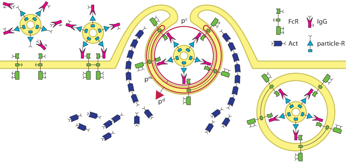
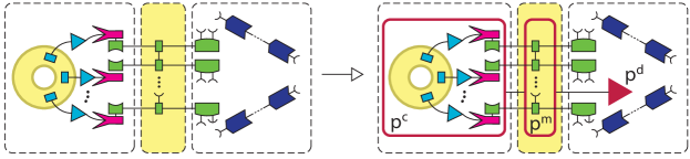
Figure 12: Fc receptor-mediated phagocytosis of an IgG-opsonized particle.

6 Conclusions

In this paper we have presented a framework for protein and membrane interactions, based on Milner’s bigraphs. Assuming the protein-level interactions as the fundamental machine, we have characterized formally a class of link graphs and their reactive systems which correspond exactly to protein solutions and protein transition systems definable in the $\kappa$-calculus [14]. Then we have extended our approach to the membrane machine, whose mobility activity can be rendered just by two fixed rules. As example applications of this framework, we have modelled the formation of vesicles, and the Fc receptor-mediated phagocytosis, giving a formal justification at protein-level of membrane-level actions.

Related and future work.

The idea of representing biological systems using bigraphs goes back to Cardelli and Milner [6, 18]. To our knowledge our framework is the first “foundational metamodel”, adequate at the protein-level, and allowing to describe formally the relations between biological models at different abstraction levels, according to the “tower of models” vision.

Damgaard et al. have developed the $\mathcal{C}$-calculus [13], an interesting language for modelling interactions of membranes and proteins. There are many relevant differences between biobigraphs and the $\mathcal{C}$-calculus. First, the $\mathcal{C}$-calculus is focused on protein diffusion through “channels”, and it does not allow for phagocytosis as the one described using biobigraphs in Section 5.2. Moreover, one of the aim of biobigraphs is to explain higher-level interactions with lower-level reactions, according to the “tower of models” vision, and to be adequate with respect to the $\kappa$-calculus. According to this vision, in biobigraphs membrane reconfigurations are logically diffent from protein reactions, but the connection between the two aspects is formally specified. In the $\mathcal{C}$-calculus, mobility and protein reactions are more intertwined, and a formal connection between $\mathcal{C}$-calculus and $\kappa$-calculus has not been investigated yet.

In fact, we can say that our approach is model-driven, that is, we have striven for an adequate (bigraphical) model before defining any language. In fact, in [3] we present Bio$\beta$, a new (meta-)language inspired and corresponding to the bigraphical framework presented in this paper, and covering both protein and membrane aspects. This language can be given an efficient, ad hoc implementation.

A stochastic version of bigraphical reactive systems has been introduced in [16], for which systems biology is indicated as the primary application. Our work is complementary, and orthogonal, to [16]; indeed, we can easily think of “stochastic biobigraphs”, endowing rules with rates, for dealing also with quantitative aspects, like reaction speeds, concentration ratios, etc., and eventually also the gene machine, in the line of recent approaches [9, 11].

Another interesting aspect to investigate is the bisimilarity definable via the IPO construction on bigraphs [18], which is always a congruence. This can be useful e.g. in synthetic biology, for instance, to verify if a synthetic protein (or even a subsystem to be implanted) behaves as the natural one.

Appendix A BiLog: a spatial logic for bigraphs

In this section we recall the main definitions and results about BiLog. For a detailed survey see [12].

BiLog is a logic for describing the structure and sub-structure of bigraphs. The models of this logic are formed by terms: the elementary terms ($\Omega$) are defined by providing a set of unary constructors ($\Theta$), then the more complex terms are constructed by composition ($\circ$) and tensor product ($\otimes$).

$$\Omega ::=id_{I}\mid\dots \Omega\in\Theta$$ (for every )

$$A,B ::=\mathbf{F}\mid A\Rightarrow B\mid id\mid\Omega\mid A\otimes B\mid A\circ B\mid A\mathbin{\circ\kern-1.50696pt-}B\mid A\mathbin{\otimes\kern-1.50696pt-}B$$

Terms are considered up to the following structural congruence $\equiv$:

$$G\equiv G\qquad G\equiv F\Rightarrow F\equiv G\qquad G\equiv G^{\prime}\wedge F\equiv F^{\prime}\Rightarrow G\circ F\equiv G^{\prime}\circ F^{\prime}$$

$$G\equiv F\wedge F\equiv H\Rightarrow G\equiv H\qquad G\equiv G^{\prime}\wedge F\equiv F^{\prime}\Rightarrow G\otimes F\equiv G^{\prime}\otimes F^{\prime}$$

$$G\circ id_{I}\equiv id_{J}\circ G\qquad(G\circ F)\circ H\equiv G\circ(F\circ H)$$

$$id_{I}\otimes id_{j}\equiv id_{I\otimes J}\qquad(G\otimes F)\otimes H\equiv G\otimes(F\otimes H)\qquad G\otimes id_{\epsilon}\equiv G\equiv id_{\epsilon}\otimes G$$

$$(G_{0}\otimes F_{0})\circ(G_{1}\otimes F_{1})\equiv(G_{0}\circ G_{1})\otimes(F_{0}\circ F_{1})$$

The logic semantics is defined as follows:

$$G\vDash\mathbf{F} {}\iff{}$$ never

$$G\vDash\Omega {}\iff{} G\equiv\Omega$$

$$G\vDash id {}\iff{} \exists I.\;G\equiv id_{I}$$

$$G\vDash A\Rightarrow B {}\iff{} \text{if }G\vDash A\text{ then }G\vDash B$$

$$G\vDash A\circ B {}\iff{} \exists G^{\prime},G^{\prime\prime}.\ G\equiv G^{\prime}\circ G^{\prime\prime}\wedge G^{\prime}\vDash A\wedge G^{\prime\prime}\vDash B$$

$$G\vDash A\otimes B {}\iff{} \exists G^{\prime},G^{\prime\prime}.\;G\equiv G^{\prime}\otimes G^{\prime\prime}\wedge G^{\prime}\vDash A\wedge G^{\prime\prime}\vDash B$$

$$G\vDash A\mathbin{\circ\kern-1.50696pt-}B {}\iff{} \forall G^{\prime}.\;\text{if }G^{\prime}\vDash A\text{ and }(G^{\prime}\circ G)\text{ is defined, then }G^{\prime}\circ G\vDash B$$

$$G\vDash A\mathbin{\otimes\kern-1.50696pt-}B {}\iff{} \forall G^{\prime}.\;\text{if }G^{\prime}\vDash A\text{ and }(G^{\prime}\otimes G)\text{ id defined, then }G^{\prime}\otimes G\vDash B$$

This kind of logic assigns to each constructor in $\Theta$ a logic constant $\Omega$ whose meaning is simply to be congruent to the corresponding constructor. The formula for the horizontal decomposition $A\otimes B$ is satisfied whenever the term can be split using a tensor product in two sub-terms whose satisfies $A$ and $B$, respectively. Recall that the tensor product does not allow the sharing of anything between two terms, this fact is quite important when we will instantiate the logic to link graphs (as we will see later on). The formula for the vertical decomposition $A\circ B$ is satisfied whenever the term ca be decomposed in an upper part and a below one (that if composed give back the original term) whose satisfies $A$ and $B$, respectively. The adjoints for composition ($\mathbin{\circ\kern-1.50696pt-}$) and tensor ($\mathbin{\otimes\kern-1.50696pt-}$) are considered.

Theorem A.1 (Logic Equivalence).

Let $G$ and $F$ be two terms.

1. $G\vDash A$ and $G\equiv H$ then $F\vDash A$.

2. $G=_{L}F$ iff $G\equiv F$;

where $=_{L}$ is the equivalence relation induced by the equisatisfiability of two terms.

Using the basic operators, we can define the following derived ones:

$$A_{I}\triangleq A\circ id_{I}\qquad A_{\rightarrow J}\triangleq id_{J}\circ A\qquad A_{I\rightarrow J}\triangleq(A_{I})_{\rightarrow J}\qquad A\circ_{I}B\triangleq A\circ id_{I}\circ B$$

$$A\mathbin{\circ\kern-1.50696pt-}_{J}B\triangleq A_{\rightarrow J}\mathbin{\circ\kern-1.50696pt-}B\qquad A\ominus B\triangleq\neg(\neg A\otimes\neg B)\qquad A\bullet B\triangleq\neg(\neg A\circ\neg B)$$

$$A^{\exists\otimes}\triangleq\mathbf{T}\otimes A\otimes\mathbf{T}\quad A^{\forall\otimes}\triangleq\mathbf{F}\ominus A\ominus\mathbf{F}\quad A^{\exists\circ}\triangleq\mathbf{T}\circ A\circ\mathbf{T}\quad A^{\forall\circ}\triangleq\mathbf{F}\bullet A\bullet\mathbf{F}$$

Intuitively, a link graph satisfies:

• $A^{\exists\otimes}$ iff it can be decomposed in some horizontal (i.e., tensorial) components, at least one of which satisfies $A$; similarly for $A^{\exists\circ}$ and vertical decomposition.

• $A^{\forall\otimes}$ iff all possible horizontal decompositions have a component satisfying $A$; similarly for $A^{\forall\circ}$ and vertical decomposition.

Logic for Link Graphs For instantiating the logic on link graphs we consider the following set of constructor:

$$\Theta_{L}=\{id_{a}:a\to a,\ /a{:\,}\mathsf{t}\colon\{a\}\rightarrow\emptyset,\ a/X\colon X\rightarrow a,\ K_{\vec{a}}\colon\emptyset\rightarrow\vec{a}\}$$

Given a signature $\langle\mathcal{K},ar,\mathcal{E}\rangle$. The constructor $/a{:\,}\mathsf{t}$ maps the name $a$ into an edge of type $\mathsf{t}\in\mathcal{E}$. $a/X$ maps all the names in $X$ to $a$, it is rather interesting to note that the special case $a/\emptyset$ (or simply $a$) represent the introduction of the name $a$. Let $K\in\mathcal{K}$ with arity $ar(K)=|\vec{a}|$ we introduce the constructor $K_{\vec{a}}\colon\emptyset\rightarrow\vec{a}$, that links the ports of $K$ to the names in $\vec{a}$.

Now, we have to extend the structural congruence $\equiv$ for covering the new constructors by adding the following axioms:

$$a/a\equiv id_{a}\qquad/a{:\,}\mathsf{t}\circ a/b\equiv/b{:\,}\mathsf{t}\qquad/a{:\,}\mathsf{t}\circ a\equiv id_{\epsilon}\qquad$$

$$b/(Y\uplus a)\circ(id_{Y}\otimes a/X)\equiv b/Y\uplus X\qquad\alpha\circ K_{\vec{a}}\equiv K_{\alpha(\vec{a})}\qquad(\text{$\alpha$ is a renaming})$$

To model properly the names (and hence the edges) of a link graphs we have to introduce the fresh name quantifier $\reversen$, very similar to the one defined in Nominal Logic. The semantics of $\reversen$ is defined as follows:

$$G\vDash\reversen x_{1}\ldots x_{n}.\;A\iff\exists a_{1}\ldots a_{n}\notin fn(G)\cup fn(A).\;G\vDash A\{x_{1}/a_{1}\dots x_{n}/a_{n}\}$$

Using the quantification on fresh names is possible to define a “separation” that shares at most a specified set of names, e.g., as the tensorial decomposition of two terms sharing the names $\vec{a}$:

$$A\stackrel{{\scriptstyle\vec{a}}}{{\otimes}}B\triangleq(\reversen\vec{x}.\;(a_{1}/\{x_{1},a_{1}\}\otimes\dots\otimes a_{n}/\{x_{n},a_{n}\})\otimes id)\circ\Big{(}\big{(}((x_{1}/a_{1}\otimes\dots\otimes x_{n}/a_{n})\otimes id)\circ A\big{)}\otimes B\Big{)}$$

Notice that this predicate has been extensively used in the definition of our sortings on the categories Lgp and BioBg.

Logic for Place Graphs For instantiating the logic on place graphs we consider the following set of constructor:

$$\Theta_{P}=\{id_{n}\colon n\rightarrow n,\ \mathbf{1}\colon 0\rightarrow 1,\ join\colon 2\rightarrow 1,\ \gamma_{1,1}\colon 2\rightarrow 2\}$$

The constructor $\mathbf{1}$ denotes the empty location. $join$ maps to location into one. Finally, $\gamma_{1,1}$ swap the left location with the right one.

As done in the case of link graphs, we extend the structural congruence ($\equiv$) for the place graph case as follows:

$$join\circ(\mathbf{1}\otimes id_{1})\equiv id_{1}\qquad\qquad join\circ\gamma_{1,1}\equiv join$$

$$join\circ(join\otimes id_{1})\equiv join\circ(id_{1}\otimes join)$$

Logic for Bigraphs It is defined by simply putting together the constructors previously introduced, formally:

$$\Theta_{B}=\{\mathbf{1}\colon\epsilon\rightarrow\langle 1,\emptyset\rangle,\,id_{\langle n,X\rangle}\colon\langle n,X\rangle\rightarrow\langle n,X\rangle,\,join\colon\langle 2,\emptyset\rangle\rightarrow\langle 1,\emptyset\rangle,\\ \gamma_{1,1}\colon\langle 2,\emptyset\rangle\rightarrow\langle 2,\emptyset\rangle,\,/a{:\,}\mathsf{t}\colon\langle 0,\,\{a\}\rangle\rightarrow\epsilon,\,a/X\colon\langle 0,X\rangle\rightarrow\langle 0,\{a\}\rangle,\,K_{\vec{a}}\colon\epsilon\rightarrow\langle 1,\vec{a}\rangle\}$$

The extension of the structural congruence ($\equiv$) is defined by the ones introduce for place and link graphs, plus the following ones, that recovers the properties of any symmetric category.

$$\gamma_{I,\epsilon}\equiv id_{I}\qquad\gamma_{I,J}\circ\gamma_{J,I}\equiv id_{I\otimes J}\qquad\gamma_{I^{\prime},J^{\prime}}\circ(G\otimes F)\equiv(F\otimes G)\circ\gamma_{I,J}$$

All the logic operators defined for the previous logics can be easily lifted to the logic of bigraphs. (They must be “lifted” on the new objects.)

Appendix B Sortings as BiLog formulae

Sortings for bigraphs are studied in [4]; in particular, a general technique for defining a safe sorting is by means of a decomposable predicate $P$, which specifies the class of morphisms we want to restrict to [4]. A predicate $P$ on morphisms is decomposable if $P(f\circ g)$ implies $P(f)$ and $P(g)$. Decomposable predicates can be conveniently denoted by BiLog formulae of the form $(\neg\phi)^{\forall\circ}$ [12], where $\phi$ characterizes unwanted morphisms. Therefore, biological bigraphs can be characterized by means of sortings specified by the corresponding BiLog formula.

In this section we will provide all the BiLog formulae for every sorting used in our framework of Biological Bigraphs.

ProtSol states that a protein solution cannot have ternary links and/or binary visible edges.

$$\ref{eq:protsol}\triangleq\big{(}\neg(K^{\prime}_{\vec{x}}\stackrel{{\scriptstyle a}}{{\otimes}}K^{\prime\prime}_{\vec{y}}\stackrel{{\scriptstyle a}}{{\otimes}}K^{\prime\prime\prime}_{\vec{z}}\otimes\mathbf{T})\big{)}^{\forall\circ}\wedge\big{(}\neg((/a{:\,}\mathsf{v}\circ K^{\prime}_{\vec{x}}\stackrel{{\scriptstyle a}}{{\otimes}}K^{\prime\prime}_{\vec{y}})\otimes\mathbf{T})\big{)}^{\forall\circ}$$

Imp says that two nodes cannot be linked if there are more than two occurrences of a membrane control along the path to the common ancestor.

$$\ref{eq:imp}\triangleq(\neg((\textrm{\sf m}^{\textrm{\sf ext}}\circ((id_{\{a\}}\mathbin{\otimes\kern-1.50696pt-}\mathbf{T})\mid(\textrm{\sf m}^{\textrm{\sf cys}}\circ\neg(a))))\stackrel{{\scriptstyle a}}{{\otimes}}\neg(a)))^{\forall\circ}.$$

Polar-Apolar forbids the nesting of nodes into locations of the same polarity:

Polar $$\triangleq\textstyle\Big{(}\neg\big{(}(\neg\mathsf{p}^{\mathsf{c}}_{y}\vee\bigvee_{K\in\{\textrm{\sf m}^{\textrm{\sf ext}}\}}K_{\vec{x}})\circ\bigvee_{K\in\mathcal{P}\uplus\{\textrm{\sf m}^{\textrm{\sf ext}}\}}K_{\vec{z}}\big{)}\Big{)}^{\forall\circ}$$

Apolar $$\triangleq\textstyle\Big{(}\neg\big{(}(\neg\mathsf{p}^{\mathsf{m}}_{y}\vee\bigvee_{K\in\{\textrm{\sf m}^{\textrm{\sf cys}}\}}K_{\vec{x}})\circ\bigvee_{K\in\mathcal{A}\uplus\{\textrm{\sf m}^{\textrm{\sf cys}}\}}K_{\vec{z}}\big{)}\Big{)}^{\forall\circ}$$

2Layer enforces the well-nesting of cells.

$$\ref{eq:bi-layer}\triangleq\Big{(}\neg\big{(}\textrm{\sf m}^{\textrm{\sf ext}}\circ((\textrm{\sf m}^{\textrm{\sf cys}}\mid\textrm{\sf m}^{\textrm{\sf cys}}\mid\mathbf{id}_{1})\vee\neg(\textrm{\sf m}^{\textrm{\sf cys}}\mid\mathbf{id}_{1}))\big{)}\Big{)}^{\forall\circ}$$

Mobil forbids that a mobility node can be peered with a protein node, forcing it to be linked with another mobility node of the same type ($P$ or $F$).

$$\ref{eq:mob}\triangleq{} \Big{(}\textstyle\neg((\bigvee_{\begin{subarray}{c}K\in\mathcal{P}\cup\mathcal{A}\\ K^{\prime}\notin\mathcal{P}\cup\mathcal{A}\end{subarray}}K_{\vec{x}}\stackrel{{\scriptstyle a}}{{\otimes}}K^{\prime}_{\vec{y}}))\wedge\neg((\bigvee_{\begin{subarray}{c}M\in\mathcal{M}\\ t\in\{\mathsf{h},\mathsf{v}\}\end{subarray}}/z{:\,}t\circ M_{\vec{z}}))\wedge\neg((\bigvee_{\begin{subarray}{c}P\in\mathcal{M}_{P}\\ F\in\mathcal{M}_{F}\end{subarray}}P_{\vec{w}}\stackrel{{\scriptstyle b}}{{\otimes}}F_{\vec{k}})\Big{)}^{\forall\circ}\wedge{}$$

$$\Big{(}\neg\big{(}\bigvee_{M\in\mathcal{M}}M_{\vec{x}}\stackrel{{\scriptstyle a}}{{\otimes}}M_{\vec{x}}\big{)}\wedge\neg\big{(}\bigvee_{\mathsf{t}\in\{\mathsf{p},\mathsf{f}\}}(\mathsf{t}^{\mathsf{c}}_{a}\stackrel{{\scriptstyle a}}{{\otimes}}\mathsf{t}^{\mathsf{d}}_{a})\vee(\mathsf{t}^{\mathsf{m}}_{xa}\stackrel{{\scriptstyle a}}{{\otimes}}\mathsf{t}^{\mathsf{c}}_{a})\vee(\mathsf{t}^{\mathsf{m}}_{ay}\stackrel{{\scriptstyle a}}{{\otimes}}\mathsf{t}^{\mathsf{d}}_{a})\big{)}\Big{)}^{\forall\circ}$$

Dir disallows mobility controls $\mathsf{p}^{\mathsf{c}}$, $\mathsf{p}^{\mathsf{d}}$, $\mathsf{f}^{\mathsf{c}}$, $\mathsf{f}^{\mathsf{d}}$ to reside in the same location.

$$\ref{eq:dir}\triangleq{}\big{(}\neg(join\circ(\mathsf{p}^{\mathsf{c}}_{x}\otimes\mathsf{p}^{\mathsf{d}}_{y})\parallel\mathsf{p}^{\mathsf{m}}_{xy})\big{)}^{\forall\circ}\wedge\big{(}\neg(join\circ(\mathsf{f}^{\mathsf{c}}_{x}\otimes\mathsf{f}^{\mathsf{d}}_{y})\parallel\mathsf{f}^{\mathsf{m}}_{xy})\big{)}^{\forall\circ}$$

NoNesting ensures the mobility actions are not nested.

$$\ref{eq:nonest}\triangleq\big{(}\textstyle(\bigvee_{m\in\{\mathsf{p}^{\mathsf{c}},\mathsf{p}^{\mathsf{m}},\mathsf{f}^{\mathsf{c}}\}}m_{\vec{x}})\circ\mathbf{T}\circ(\bigvee_{m\in\mathcal{M}}m_{\vec{y}})\big{)}^{\forall\circ}$$

Fuse ensures well-defined fusions.

$$\ref{eq:fuse}\triangleq\big{(}\textstyle\neg(\mathsf{f}^{\mathsf{c}}\circ(\textrm{\sf m}^{\textrm{\sf ext}}\otimes\textrm{\sf m}^{\textrm{\sf ext}}\otimes\mathbf{T})\vee\mathsf{f}^{\mathsf{c}}\circ(\bigvee_{K\in\mathcal{P}\cup\mathcal{A}}K_{\vec{x}}\otimes\mathbf{T}))\big{)}^{\forall\circ}$$

References

- [1] A. Aderem and D. M. Underhill. Mechanisms of phagocytosis in macrophages. Annual Review of Immunology, 17(1):593–623, 1999. PMID: 10358769.
- [2] B. Alberts, D. Bray, K. Hopkin, A. Johnson, J. Lewis, M. Raff, K. Roberts, and P. Walter. Essential Cell Biology, 2nd edition. Garland, 2003.
- [3] G. Bacci, D. Grohmann, and M. Miculan. A framework for protein and membrane interactions. In G. Ciobanu, editor, Proc. MeCBIC’09, EPTCS, 2009.
- [4] L. Birkedal, S. Debois, and T. T. Hildebrandt. On the construction of sorted reactive systems. In F. van Breugel and M. Chechik, editors, Proc. CONCUR, LNCS 5201, pages 218–232. Springer, 2008.
- [5] M. Bundgaard and V. Sassone. Typed polyadic pi-calculus in bigraphs. In Proc. PPDP, pages 1–12. 2006.
- [6] L. Cardelli. Bioware languages. In K. S. J. Andrew Herbert, editor, Computer Systems: Theory, Technology, and Applications - A Tribute to Roger Needham, pages 59–65. Springer, 2004.
- [7] L. Cardelli. Brane calculi. In Proc. CMSB, LNCS 3082, pages 257–278. Springer, 2004.
- [8] L. Cardelli. Abstract machines of systems biology. T. Comp. Sys. Biology, 3737:145–168, 2005.
- [9] L. Cardelli. A process algebra master equation. In Proc. QEST, pages 219–226. IEEE, 2007.
- [10] L. Cardelli. Bitonal membrane systems: Interactions of biological membranes. Theoretical Computer Science, 404(1-2):5 – 18, 2008. Membrane Computing and Biologically Inspired Process Calculi.
- [11] F. Ciocchetta and J. Hillston. Process algebras in systems biology. In M. Bernardo, P. Degano, and G. Zavattaro, editors, Proc. SFM, LNCS 5016, pages 265–312. Springer, 2008.
- [12] G. Conforti, D. Macedonio, and V. Sassone. Spatial logics for bigraphs. In L. Caires, G. F. Italiano, L. Monteiro, C. Palamidessi, and M. Yung, editors, Proc. ICALP, volume 3580 of Lecture Notes in Computer Science, pages 766–778. Springer, 2005.
- [13] T. C. Damgaard, V. Danos, and J. Krivine. A language for the cell. Technical Report TR-2008-116, IT University of Copenhagen, Dec. 2008.
- [14] V. Danos and C. Laneve. Formal molecular biology. Theoretical Computer Science, 325, 2004.
- [15] E. Garcia-Garcia and C. Rosales. Signal transduction during fc receptor-mediated phagocytosis. J. Leukocyte Biology, 72(6):1092–1108, 2002.
- [16] J. Krivine, R. Milner, and A. Troina. Stochastic bigraphs. In Proc. 24th MFPS, ENTCS 218:73–96, 2008.
- [17] J. J. Leifer and R. Milner. Deriving bisimulation congruences for reactive systems. In C. Palamidessi, editor, Proc. CONCUR, volume 1877 of Lecture Notes in Computer Science, pages 243–258. Springer, 2000.
- [18] R. Milner. Pure bigraphs: Structure and dynamics. Information and Computation, 204(1):60–122, 2006.
- [19] R. Milner. The tower of informatic models. In From semantics to Computer Science; Essays in Memory of Gilles Kahn. Cambridge University Press, 2009.