$\Lambda_{QCD}$ from gluon and ghost propagators

Abstract:

Fundamental quantities of QCD, such as the strong coupling and $\Lambda_{QCD}$, are studied in the framework of lattice QCD with $N_{f}=2$ twisted mass fermions. In particular, the contact between lattice and continuous calculations is made by comparing the renormalized ghost-gluon vertex in MOM scheme with 4-loop perturbative results. A power correction is needed in order to have agreement between the two descriptions. This suggests the presence of a dimension-two $\left\langle{A^{2}}\right\rangle$ gluon condensate whose value is found to be higher than in the quanched case.

1 Introduction

The lattice provides a very elegant way of calculating renormalized observables. In this framework several methods are known to extract the running of the QCD coupling constant, which allows for the determination of the QCD scale, $\Lambda_{QCD}$ and for the study of infrared properties. In the case of quenched world the mismatch between the perturbative running and the lattice one has revealed the presence of a non-null gluon condensate of dimension two that, being non-gauge invariant, has motivated the research of its possible implications for the gauge-invariant world.

In this note we apply the already established methods for $N_{f}=2$ dynamical quarks, including light up and down quarks. $N_{f}=2+1+1$ lattice simulations are already being performed, thus a realistic lattice estimate of $\Lambda_{\overline{MS}}$ directly comparable with experimental results will become inmediatly accesible.

In particular here we focus on the study of the ghost-gluon vertex in the configuration of vanishing incoming ghost-momentum. Only in this case the ghost-gluon vertex can be related directly to the bare and ghost propagators, making calculations simpler.

2 Taylor scheme

2.1 Definitions

In [1] was shown that the so-called Taylor scheme is the only one where the coupling can be cumputed from two-point Green functions, due to Taylor’s theorem. We write Landau gauge gluon and ghost propagators as:

$$\left(G^{(2)}\right)_{\mu\nu}^{ab}(p^{2},\Lambda) = \frac{G(p^{2},\Lambda)}{p^{2}}\ \delta_{ab}\left(\delta_{\mu\nu}-\frac{p_{\mu}p_{\nu}}{p^{2}}\right)\ ,$$

$$\left(F^{(2)}\right)^{a,b}(p^{2},\Lambda) = -\delta_{ab}\ \frac{F(p^{2},\Lambda)}{p^{2}}\ ;$$ (1)

with $\Lambda$ the regularisation cutoff. The renormalized dressing functions, $G_{R}$ and $F_{R}$ are defined through :

$$G_{R}(p^{2},\mu^{2})\ = \ \lim_{\Lambda\to\infty}Z_{3}^{-1}(\mu^{2},\Lambda)\ G(p^{2},\Lambda)$$

$$F_{R}(p^{2},\mu^{2})\ = \ \lim_{\Lambda\to\infty}\widetilde{Z}_{3}^{-1}(\mu^{2},\Lambda)\ F(p^{2},\Lambda)\ ,$$ (2)

with MOM renormalization condition

$$G_{R}(\mu^{2},\mu^{2})=F_{R}(\mu^{2},\mu^{2})=1\ .$$ (3)

Due to Taylor’s non-renormalization theorem, the renormalized coupling defined from the ghost-gluon vertex with a zero incoming ghost momentum can be computed from ghost and gluon propagators using:

$$\alpha_{T}(\mu^{2})\equiv\frac{g^{2}_{T}(\mu^{2})}{4\pi}=\ \lim_{\Lambda\to\infty}\frac{g_{0}^{2}(\Lambda^{2})}{4\pi}G(\mu^{2},\Lambda^{2})F^{2}(\mu^{2},\Lambda^{2})\ ;$$ (4)

what has been called Taylor  scheme [1]

2.2 Perturbation theory and OPE

The perturbative running of $\alpha_{T}$ is known up to four loops [2],

$$\alpha_{T}(\mu^{2}) = \frac{4\pi}{\beta_{0}t}\left(1-\frac{\beta_{1}}{\beta_{0}^{2}}\frac{\log(t)}{t}+\frac{\beta_{1}^{2}}{\beta_{0}^{4}}\frac{1}{t^{2}}\left(\left(\log(t)-\frac{1}{2}\right)^{2}+\frac{\widetilde{\beta}_{2}\beta_{0}}{\beta_{1}^{2}}-\frac{5}{4}\right)\right)$$ (5)

$$+\frac{1}{(\beta_{0}t)^{4}} \left(\frac{\widetilde{\beta}_{3}}{2\beta_{0}}+\frac{1}{2}\left(\frac{\beta_{1}}{\beta_{0}}\right)^{3}\left(-2\log^{3}(t)+5\log^{2}(t)+\left(4-6\frac{\widetilde{\beta}_{2}\beta_{0}}{\beta_{1}^{2}}\right)\log(t)-1\right)\right)$$ (6)

with $t=\ln\frac{\mu^{2}}{\Lambda_{T}^{2}}$ and the perturbative coefficients:

$$\widetilde{\beta}_{0} = \overline{\beta}_{0}=11-\frac{2}{3}N_{f}$$

$$\widetilde{\beta}_{1} = \overline{\beta}_{1}=102-\frac{38}{3}N_{f}$$

$$\widetilde{\beta}_{2} = \overline{\beta}_{2}-\overline{\beta}_{1}c_{1}+\overline{\beta}_{0}(c_{2}-c_{1}^{2})$$

$$= 3040.48\ -\ 625.387\ N_{f}\ +\ 19.3833\ N_{f}^{2}$$

$$\widetilde{\beta}_{3} = \overline{\beta}_{3}-2\overline{\beta}_{2}c_{1}+\overline{\beta}_{1}c_{1}^{2}+\overline{\beta}_{0}(2\ c_{3}-6\ c_{2}c_{1}+4\ c_{1}^{3})$$ (7)

$$= 100541\ -\ 24423.3\ N_{f}\ +\ 1625.4\ N_{f}^{2}\ -\ 27.493\ N_{f}^{3}\ ,$$

The parameters $\Lambda_{QCD}$ in two schemes can be perturbatively related at high energy. In particular, from the $T$-scheme to $\overline{MS}$ this relationship reads:

$$\frac{\Lambda_{\overline{\rm MS}}}{\Lambda_{T}}\ =\ e^{\displaystyle-\frac{c_{1}}{2\beta_{0}}}\ =\ e^{\displaystyle-\frac{507-40N_{f}}{792-48N_{f}}}\ .$$ (8)

Following the Operatore Product Expansion (OPE) program both ghost and gluon propagators show the appearance of a non-perturbative power correction driven by the non-gauge invariant dimension-two gluon condensate (see [1], [3] and referencies therein). Including power corrections at tree-level in ghost and gluon dressing functions, one can rewrite (4) as

$$\alpha_{T}(\mu^{2}) = \alpha^{\rm pert}_{T}(\mu^{2})\left(1+\frac{9}{\mu^{2}}\frac{g^{2}_{T}(q_{0}^{2})\langle A^{2}\rangle_{R,q_{0}^{2}}}{4(N_{C}^{2}-1)}\right)\ ,$$ (9)

where $q_{0}^{2}\gg\Lambda_{\rm QCD}$ is some perturbative scale and the running of the perturbative part is described by equation (5). This formula will be used for the data analysis in the next section that does depend on two parameters, $\Lambda_{QCD}$ and $\langle A^{2}\rangle$, that will be fitted.

3 Lattice setup and role of $H(4)$ orbits

The results presented here are based on the gauge field configurations generated by the European Twisted Mass Collaboration (ETMC) with the tree-level improved Symanzik gauge action [4] and the twisted mass fermionic action [5] at maximal twist, discussed in detail in refs. [6]- [9].

We preliminarly exploited 100 ETMC gauge configurations obtained for $\beta=3.9$ ($\mu=0.0085$), 60 for $\beta=4.05$ ($\mu=0.006$) and 100 for $\beta=4.2$ ($\mu=0.002$) simulated on $24^{3}\times 48$ lattices, corresponding to $N_{f}=2$ in order to compute the gauge-fixed 2-point gluon and ghost Green functions.

For fixing Landau gauge in the lattice we minimise the functional

$$F_{U}[g]=Re\sum_{x}\sum_{\mu}\left(1-\frac{1}{N}g(x)U_{\mu}(x)g(x+\mu)\right)$$ (10)

respect to the gauge transform $g$. Ghost propagator is computed in Landau gauge as the inverse of the Faddeev-Popov operator, that is written as the lattice divergence,

$$M(U)=-\frac{1}{N}\nabla\cdot\widetilde{D}(U)$$ (11)

where the operator $\widetilde{D}$ acting on an arbitrary element of the Lie algebra, $\eta$ reads:

$$\widetilde{D}(U)\eta(x)=\frac{1}{2}\left(U_{\mu}(x)\eta(x+\mu)-\eta(x)U_{\mu}(x)+\eta(x+\mu)U_{\mu}^{\dagger}-u_{\mu}^{\dagger}(x)\eta(x)\right)\ .$$ (12)

More details on the lattice procedure for the inversion of Faddeev-Popov operator can be found on [10].

As we intend to fit the running of $\alpha_{s}$, our interest is to have, on one hand the highest momenta accesible and, on the other the highest number of data points to perform the fit. When working at a given lattice spacing, the momentum window has to be limited due to the presence of high discretization errors. These lattice artifacts are due to the breaking of the rotational symmetry of the euclidean space-time when using an hypercubic lattice, where this symmetry is restricted to the discrete H(4) isometry group. These artifacts can be illustrated as the difference between the lattice momenta,

$$\tilde{p}_{\mu}=\frac{1}{a}\sin ap_{\mu}$$ (13)

and the continuum ones,

$${p}_{\mu}=\frac{2\pi n}{Na}\qquad n=0,1,\cdots,N\ .$$ (14)

Clearly these two momenta will differ except in the limit $n/N\to 0$. Following what was recently discussed in [11] and [12], let us consider an adimensional lattice correlation function $Q$ that depends on the lattice momentum $a\tilde{p}_{\mu}$ and some mass scale $a\Lambda$: $Q\equiv Q(a^{2}\tilde{p}^{2},a^{2}\Lambda^{2})$ . The lattice momentum can be developed as:

$$a^{2}\tilde{p}_{\mu}^{2}=a^{2}p_{\mu}^{2}+c_{1}a^{4}p_{\mu}^{4}+\cdots$$ (15)

with $c_{1}$ a constant that depends on the discretization chosen. Then:

$$a^{2}\tilde{p}^{2}\equiv\sum_{\mu=1}^{4}a^{2}\tilde{p}_{\mu}^{2}=a^{2}p^{2}+c_{1}a^{4}p^{[4]}+\cdots=a^{2}p^{2}\left(1+c_{1}a^{2}\frac{p^{[4]}}{p^{2}}+\cdots\right)$$ (16)

where $p^{[4]}=\sum_{\mu=1}^{4}p_{\mu}^{4}$. If the lattice spacing is small, $\epsilon=a^{2}p^{[4]}/p^{2}<<1$ and we can develop $Q$ in powers of $\epsilon$:

$$Q(a^{2}\tilde{p}_{\mu}^{2},a^{2}\Lambda^{2}) \equiv Q\left(a^{2}p^{2}\left(1+c_{1}a^{2}\frac{p^{[4]}}{p^{2}}+\cdots\right),a^{2}\Lambda^{2}\right)$$ (17)

$$= Q(a^{2}p^{2},a^{2}\Lambda^{2})+\left.\frac{dQ}{d\epsilon}\right|_{\epsilon=0}a^{2}\frac{p^{[4]}}{p^{2}}+\cdots$$ (18)

$H(4)$ methods are based on the appearance of a $\mathcal{O}(a^{2})$ corrections driven by a $p^{[4]}$ term. The basic method is to fit between the whole set of orbits sharing the same $p^{2}$ the coefficient $R$ and the extrapolated value of $Q$ free from H(4) artefacts. In particular we assumed that the coefficient

$$\left.R(a^{2}p^{2},a^{2}\Lambda^{2})=\frac{dQ\left(a^{2}p^{2}\left(1+c_{1}\epsilon+\cdots\right),a^{2}\Lambda^{2}\right)}{d\epsilon}\right|_{\epsilon=0}$$

has a smooth dependence on $a^{2}p^{2}$ over a given momentum window. This can be achieved by developing $R$ as $R=R_{0}+R_{1}a^{2}p^{2}$ and making a global fit in a momentum window between $(p-\delta,p+\delta)$ to extract the extrapolated value of $Q$ for the momentum $p$ and shifting the window for every lattice momentum. This procedure of fitting is somehow different from the previous one, since the extrapolation does not rely on any particular assumption for the functional form of $R$. On the other, the systematic error coming from the extrapolation can be estimated by modifying the width of the fitting window.

4 Results

4.1 Calibration of lattice spacings

The running of $\alpha_{T}$ given by the combination of Green functions in eq. (4) does depend in principle on the momentum and the cut-off. Nevertheless, if we are not far from the continuum limit, and discretization errors are treated properly, the coupling will depend only on the momentum (except, maybe, finite volume errors at low momenta).

The procedure to compute the ratio of lattice spacings is then straightforward: it can be obtained by requiring the estimates of $\alpha_{T}$ for two different simulations (two different $\beta$’s) to match properly each other. This method has proven to be successful in quenched lattice simulations [1], with a deviation with respect to usual Sommer parameter estimates lower than $5\%$.

The $N_{f}=2$ results can be seen in figure 1, where the lattice spacing for the lower $\beta$ ($\beta=3.9$) has been assumed to coincide with the one given in [6] and the other two, for $\beta=4.05$ and $\beta=4.20$ are fitted to match the data.

	This paper	Sommer scale	deviation (%))
$a(3.9)/a(4.05)$	1.223(3)	1.277	4.2
$a(3.9)/a(4.2)$	1.503(5)	1.547	2.9

Table 1: Best-fit parameters for the ratios of lattice spacings. The error is purely statistics.

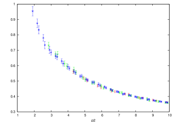
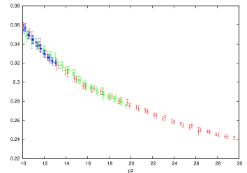
Figure 1: QCD coupling defined by from the three lattice data sets employed: red squares stand for $\beta=4.2$, green ones for $\beta=4.05$ and blue for $\beta=3.90$. Right (left) plot shows estimates for momenta above (below) 10 $GeV^{2}$. The physical value (in $GeV$) of the momentum in $x$-axis is obtained by applying the ratios of lattice sizes in tab.1 and $a(3.9)^{-1}=2.301GeV$.

The deviations are found to be smaller than $5\%$ (see Tab. 1), as in the quenched case. This deviation might be a signal of discretization errors still present at these $\beta$’s. Another source of discrepancy could be a possible dependence of results on the quark masses. Further efforts should be done in this sence.

4.2 $\Lambda_{\overline{MS}}$ and $\left\langle{A^{2}}\right\rangle$ condensate

The value of $\Lambda_{\overline{\rm MS}}$ can be obtained by inverting (5) for the lattice values of $\alpha_{T}$ obtained from the lattice for each momentum. When done (figure 2) the values of $\Lambda_{\overline{\rm MS}}$ obtained have a strong dependence on the momentum, showing the presence of some non-perturbative effects not taken into account in (5). The values of $\Lambda_{\overline{\rm MS}}$ are around $320-360{\rm MeV}$, much higher than other estimations.

The first non-perturbative correction that does appear un Landau gauge is the $\langle{A^{2}}\rangle$ gluon condensate, whose effects on the running coupling are included in (9). The values of $\Lambda_{\overline{\rm MS}}$ and $\langle{A^{2}}\rangle$ can be simultaneously fixed from lattice data using, for example, the “plateau” method, shown in [1]. It consist in varying the value of the condensate to look for a “plateau” in $\Lambda_{\overline{\rm MS}}$ over a given momentum window.

In fig. 2, we also plot $\Lambda_{\overline{\rm MS}}$ derived from confronting the lattice value of $\alpha_{T}$ with the perturbative+OPE prediction, in terms of the momentum where $\alpha_{T}$ is estimated from the lattice. The application of the “plateau” method allows us to get as a best estimate:

$$\Lambda_{\overline{\rm MS}}\ =\ 267\pm 11{\rm MeV}\ ;$$ (19)

where again the error takes into account no systematic effect. This result is in good agreement with other estimations in litteraure [13]- [15].

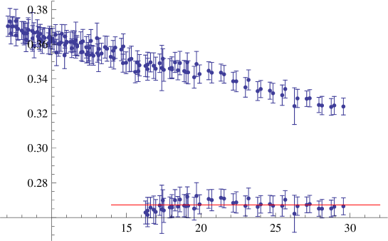
Figure 2: $\Lambda_{\overline{\rm MS}}$ derived from fitting the lattice value of $\alpha_{T}$ with the perturbative+OPE prediction, in terms of the momentum where $\alpha_{T}$ is estimated from the lattice, as described in ref. [1].

The value of the $\left\langle{A^{2}}\right\rangle$ obtained is

$$g_{T}^{2}\left\langle{A^{2}}\right\rangle_{R,\mu}=9.6\pm 0.6{\rm GeV}^{2}$$ (20)

which shows a significant increase respect to previous quenched estimates [1].

5 Conclusions and outlooks

We calculated the running coupling in the Taylor scheme with $N_{f}=2$ flavours of dynamical quarks. We found that the matching of the results obtained for different $\beta$’s allows to compute the ratio of lattice spacings, with a deviation with respect to the string tension always smaller than $5\%$.

By comparing the lattice result with the expectation coming from perturbation theory, we found the need for a dimension-two gluon condensate associated to a non-perturbative power correction. Including this term allows for an agreement between lattice and continuous formulae and then the extraction of the scale $\Lambda_{\overline{\rm MS}}^{N_{f}=2}$. Our result is in agreement with previous determinations.

The application of this method is straightforward for a higher number of quark flavours and might be used in forthcoming $N_{f}=2+1+1$ lattice simulations.

As an outlook, we are interested in checking the mass-dependence of our results. In particular two effects are to be expected. The first one, at the level of the calibration, could show a dependence of the lattice spacing both on $\beta$ and $\mu$. In any case this should not affect our results. The second one could be the effect of the mass on the coupling, which seems to be rouled out because of the good overlap of the coupling already observed at different $\mu$’s.

5.1 Acknowledgements

We thank the IN2P3 Computing Center (Lyon) where our simulations have been done.

References

- [1] Ph. Boucaud, F. De Soto, J. P. Leroy, A. Le Yaouanc, J. Micheli, O. Pene and J. Rodriguez-Quintero, Phys. Rev. D 79, 014508 (2009) [arXiv:0811.2059 [hep-ph]].
- [2] K. G. Chetyrkin, Nucl. Phys. B 710, 499 (2005) [arXiv:hep-ph/0405193].
- [3] Ph. Boucaud, A. Le Yaouanc, J. P. Leroy, J. Micheli, O. Pene and J. Rodriguez-Quintero, Rev. D 63 (2001) 114003 [arXiv:hep-ph/0101302].
- [4] P. Weisz, Nucl. Phys. B 212 (1983) 1.
- [5] R. Frezzotti, P. A. Grassi, S. Sint and P. Weisz [Alpha collaboration], JHEP 0108 (2001) 058 [arXiv:hep-lat/0101001].
- [6] Ph. Boucaud et al. [ETM Collaboration], Phys. Lett. B 650 (2007) 304 [arXiv:hep-lat/0701012].
- [7] Ph. Boucaud et al. [ETM collaboration], Comput. Phys. Commun. 179 (2008) 695 [arXiv:0803.0224 [hep-lat]].
- [8] C. Urbach [ETM Coll.], PoS LAT2007 (2007) 022 [0710.1517 [hep-lat]].
- [9] P. Dimopoulos et al. [ETM Collaboration], arXiv:0810.2873 [hep-lat].
- [10] Ph. Boucaud et al., Phys. Rev. D 72 (2005) 114503 [arXiv:hep-lat/0506031].
- [11] D. Becirevic, P. Boucaud, J. P. Leroy, J. Micheli, O. Pene, J. Rodriguez-Quintero and C. Roiesnel, Phys. Rev. D 60 (1999) 094509 [arXiv:hep-ph/9903364].
- [12] F. de Soto and C. Roiesnel, JHEP 0709 (2007) 007 [arXiv:0705.3523 [hep-lat]].
- [13] M. Gockeler, R. Horsley, A. C. Irving, D. Pleiter, P. E. L. Rakow, G. Schierholz and H. Stuben, Phys. Rev. D 73 (2006) 014513 [arXiv:hep-ph/0502212].
- [14] A. Sternbeck, K. Maltman, L. von Smekal, A. G. Williams, E. M. Ilgenfritz and M. Muller-Preussker, PoS LAT2007 (2007) 256 [arXiv:0710.2965 [hep-lat]].
- [15] M. Della Morte, R. Frezzotti, J. Heitger, J. Rolf, R. Sommer and U. Wolff [ALPHA Collaboration], Nucl. Phys. B 713 (2005) 378 [arXiv:hep-lat/0411025].