The atomic approach of the Anderson model for the U finite case: application to a quantum dot

Abstract

In the present work we apply the atomic approach to the single impurity Anderson model (SIAM). A general formulation of this approach, that can be applied both to the impurity and to the lattice Anderson Hamiltonian, was developed in a previous work (arXiv:0903.0139v1 [cond-mat.str-el]). The method starts from the cumulant expansion of the periodic Anderson model (PAM), employing the hybridization as perturbation. The atomic Anderson limit is analytically solved and its sixteen eigenenergies and eigenstates are obtained. This atomic Anderson solution, which we call the (AAS), has all the fundamental excitations that generate the Kondo effect, and in the atomic approach is employed as a “seed ” to generate the approximate solutions for finite $U$. The width of the conduction band is reduced to zero in the AAS, and we choose its position so that the Friedel sum rule (FSR) be satisfied, close to the chemical potential $\mu$.

We perform a complete study of the density of states of the SIAM in all the relevant range of parameters: the empty dot, the intermediate valence (IV-regime),the Kondo and the magnetic regime. In the Kondo regime we obtain a density of states that characterizes well the structure of the Kondo peak. To shown the usefulness of the method we have calculated the conductance of a quantum dot, side coupled to a conduction band.

I Introduction

Experimental results indicate Clogston that localized magnetic moments could appear when magnetic impurities are dissolved in a metal, and a minimum in the electrical resistivity is always present in the material at low temperatures $T$. Jun Kondo was the first who associated the formation of magnetic moments in the material with the minimum of the resistivity. He studied the phenomena employing perturbation theory in second order in the Born approximation, Kondo64 and showed that the minimum was generated by the spin-flip scattering of the conduction electrons with the magnetic moment of the impurity; this phenomena become known as the Kondo effect. In its calculation Kondo showed that the resistivity increases with the decrease of temperature according to $ln(T)$, which become known as the logarithmic divergence of the Kondo effect. In the alloys formed in such a way it is not possible to control the Kondo parameters microscopically, but with the advent of nanotechnology the Kondo effect was realized experimentally in quantum dots (QD), with complete control over all the relevant parameters Goldhaber98 .

Quantum dots are artificial atoms that offer a high degree of parameter control by means of simple gate electrostatics, allowing the nanometric confinement of the electrons. The coupling between the quantum dot and the electronic reservoirs produces tunneling events that can modify the discrete energy levels of the dot, changing them into complicated many-body wave functions. When conducting electrons move in an out the nanostructure, a progressive screening of the atomic spin occurs, in complete analogy with the well-known Kondo effect in solids containing magnetic impurities. The Kondo effect in quantum dots is then observed as a zero-bias conductance resonance, associated with the entangled state of the electrons in the electronic reservoirs and in the dot.

The experimental realization of the Kondo effect in QD’s renewed the interest in searching new approximate solutions for the single impurity Anderson model (SIAM) and several calculations of the Green’s functions (GF) employing the method of motion equation (EOM) were reconsidered, Meir93 ; Luo99 but such methods suffered several drawbacks due to their failure to satisfy the completeness and the Friedel sum rule. Completeness07 Another method that was extensively applied to describe the SIAM is the slave boson mean field theory, Coleman1 but this method suffered from a spurious second order phase transition. X-boson1 Another recent approach that describes the SIAM is the local moment approach, Logan98 that satisfies a number of correct limits: weak-coupling Fermi liquid, atomic limit, and the Kondo regime, but the strong coupling limit is plagued with a symmetry breaking and an unphysical static order value of the local magnetic moment. Very recently appeared an analytical calculation, Janis08 that employed diagrammatic expansions with Feynman diagrams and obtained the Kondo resonance in the electron-hole symmetric limit, but out of this limit the Kondo resonance was lost. Another appealing approach is the quantum Monte Carlo technique, Monte_Carlo that is expensive from the computational point of view and is restricted from intermediate to high temperatures. Other expensive computational numerical methods are the dynamical mean field theory (DMFT) Kraut and the density-matrix renormalization group (DMRG). Schollwock2005 The most effective approach which nowadays describes the dynamical properties of the SIAM is the numerical renormalization group (NRG), NRG1 ; NRG2 ; NRG3 but as the other powerful methods it is expensive from the numerical point of view and presents some limitations; the NRG describes very well the Kondo Physics but presents convergence problems in the extreme Kondo limit. Costi96 Until now it was missing a dynamical theory that describes the transition from the weak coupling limit $U<<\Delta$ to the strong coupling limit $U>>\Delta$, where $U$ is the Coulomb repulsion and $\Delta=\pi V^{2}\rho_{c}$, and $V$ is the hybridization and $\rho_{c}$ is the density of states of the conduction electrons.

The main objective of this paper is to fill the gap described above: the atomic approach is able to describe quantitatively all the regimes of the SIAM in the weak, intermediate and strong correlation limits of the model. Due to the simplicity of its implementation (practically all the method is analytical) and very low computational cost (a density of states curve can be obtained in few seconds or less), the atomic approach is a good candidate to describe strongly correlated impurity systems that exhibits the Kondo effect, like quantum dots Thiago1_2006 or carbon nanotubes. Thiago2_2006 The atomic approach does not substitute powerful computational methods like NRG,DMFT or DMRG, but can be a first choice to describe systems where the Kondo physics is relevant. In an earlier work Thiago06 we developed the atomic approach for the strong coupling limit ($U\rightarrow\infty$), and in the present work we present the atomic approach for finite U.

The Kondo effect for both the impurity and the lattice are described by the Anderson Hamiltonian, which considers systems that have two types of electrons: the localized electrons ($f$-electrons), that are strongly correlated, and the conduction electrons ($c$-electrons), that can be described as free. The Anderson model allows the interchange between the $f$ and the $c$ electrons through the hybridization interaction, and to study this problem we shall consider the cumulant expansion of the periodic Anderson model (PAM) employing the hybridization as perturbation. FFM From the cumulant expansion we obtain formal expressions for the exact one-electron Green’s functions (GF) in terms of effective cumulants, that are as difficult to calculate as the exact GF, and our approximation consists in substituting these effective cumulants by those of the atomic case of the Anderson model, that is exactly soluble. In general the Anderson model does not have analytical solutions, but when the energies of all the $N$ conduction states have collapsed (the conduction band has zero width) and the hybridization is local (i.e. independent of the wave vector $\mathbf{k}$), the Anderson Hamiltonian has an exact solution, and the electronic Green’s functions can be calculated analytically. In this case it is only necessary to study a single site, that can hold up to four electrons: two $f$-electrons and two $c$-electrons. With the $f$-electrons we can build four states: one $\mid 0\rangle$ with no electrons, two with one electron with spin up$\mid+\rangle$ or with spin down$\mid-\rangle$ and one $\mid d\rangle$ with the two electrons at the same site. In a similar way we can build up four states $\mid 0\rangle,\mid\uparrow\rangle,\mid\downarrow\rangle,\mid\uparrow\downarrow\rangle$ with the $c$-electrons, and for a given site we have then a vector space of dimension sixteen. The corresponding Anderson Hamiltonian is then easily diagonalized, giving sixteen eigenenergies and eigenstates that we shall name the atomic Anderson solution (AAS), and this minimal Anderson system contains already the fundamental excitations that generate the Kondo effect. To chose the position of the conduction band of the AAS, we impose the satisfaction of Friedel’s sum rule.

In Sec. II we present a brief review of the basic equations of the atomic approach formalism developed in an earlier publication. RMP In Sec. III we discuss in detail the equations and approximations employed in the development of the atomic approach. In Sec. IV we define the completeness and calculate the occupation numbers. In Sec. V we discuss what criteria we shall use to determine the parameters of the AAS: the satisfaction of the completeness or the Friedel sum rule. We also present a discussion of the emergence of the Kondo peak from the weak to the strong coupling regime. In Sec. VI we present the results of the formation of the Kondo peak for a fixed $E_{f}$ level and variable correlation $U$. In Sec. VII we fix the correlation $U$ and vary the $E_{f}$ level describing the empty dot, the intermediate valence (IV), the Kondo and the magnetic regimes. To show the usefulness of the atomic approach, we calculate in Sec. VIII the conductance of a side coupled QD. QDnosso ; Kobayashy2004 In Sec. VIII we present the conclusions of the work and in the appendix A we give the details of the analytic calculation of the exact Green’s function in the limit of zero conduction bandwidth, as well as the relevant atomic Green’s functions.

II The Anderson Hamiltonian

In this section we present a brief review of the basic equations of the atomic approach formalism developed in an earlier publication RMP . The Hamiltonian for the Anderson lattice with finite U is given by

$$H =\sum_{\vec{k},\sigma}E_{\mathbf{k},\sigma}C_{\mathbf{k},\sigma}^{\dagger}C_{\mathbf{k},\sigma}+\sum_{j,\sigma}E_{\sigma\ }f_{j,\sigma}^{\dagger}f_{j,\sigma}$$ (1)

$$+U\sum_{j}n_{j,\sigma}n_{j,\overline{\sigma}}+H_{h},$$

where the operators $C_{\mathbf{k},\sigma}^{\dagger}$ and $C_{\mathbf{k},\sigma}$ are the creation and destruction operators of the conduction band electrons (c-electrons) with wave vector $\mathbf{k}$, component of spin $\sigma$ and energies $E_{\mathbf{k},\sigma}$. The $f_{i,\sigma}^{\dagger}$ and $f_{i,\sigma}$ are the corresponding operators for the $f$-electrons in the Wannier localized state at site j, with site independent energy $E_{\sigma}$ and spin component $\sigma$. The third term is the Coulomb repulsion between the localized electrons at each site, where $n_{j,\sigma}=f_{j,\sigma}^{\dagger}f_{j,\sigma}$ is the number of $f$-electrons with spin component $\sigma$ at site $j$ and the symbol $\overline{\sigma}$ denotes the spin component opposite to $\sigma$. The fourth term $H_{h}$ describes the hybridization between the localized and conduction electrons

$$H_{h}=\sum_{j,\mathbf{k},\sigma}(V_{j,\mathbf{k},\sigma}f_{j,\sigma}^{\dagger}C_{\mathbf{k},\sigma}+V_{j,\mathbf{k},\sigma}^{\ast}C_{\mathbf{k},\sigma}^{\dagger}f_{j,\sigma}).$$ (2)

The hybridization constant $V_{j,\mathbf{k},\sigma}$ in this equation is given by

$$V_{j,\mathbf{k},\sigma}=\frac{1}{\sqrt{N_{s}}}V_{\sigma}(\mathbf{k})\exp{(i\mathbf{k}.\mathbf{R}_{j}),}$$ (3)

and when the Hubbard operators are introduced into Eq. (2) , the hybridization Hamiltonian $H_{h}$ is transformed into:

$$H_{h}=\sum_{jba,\mathbf{k}\sigma}\left(V_{jba,\mathbf{k}\sigma}X_{j,ba}^{\dagger}C_{\mathbf{k}\sigma}+V_{jba,\mathbf{k}\sigma}^{\ast}C_{\mathbf{k}\sigma}^{\dagger}X_{j,ba}\right),$$ (4)

where the label $\alpha=(b,a)$ in $H_{h}$ describes the transition $\mid a>\rightarrow\mid b>$, and the local state $\mid a>$ has one electron more than the state $\mid b>$. There are four local states $\mid 0>$, $\mid+>$, $\mid->$ and $\mid d>=\mid+,->$ per site, and there are only four $X$ operators that destroy one local electron at a given site.

The identity relation in the reduced space of the localized states at site $j$ is

$$X_{j,oo}+X_{j,\sigma\sigma}+X_{j,\overline{\sigma}\overline{\sigma}}+X_{j,dd}=I,$$ (5)

where $\overline{\sigma}=-\sigma$, and the four $X_{f,aa}$ are the projectors into the corresponding states $\mid f,a\rangle$. The occupation numbers on the impurity $n_{f,a}=<X_{f,aa}>$ satisfy the “completeness” relation

$$n_{f,0}+n_{f,\sigma}+n_{f,\overline{\sigma}}+n_{f,d}=1.$$ (6)

We use the index $I_{x}=1,2,3,4$, defined in Table I, to characterize these $X$ operators:

$I_{x}$	$1$	$2$	$3$	$4$
$\alpha=(b,a)$	$(0,+)$	$(0,-)$	$(-,d)$	$(+,d)$

Table 1: Representation of the possible transitions present in the finite $U$ atomic SIAM Hamiltonian. $I_{x}=1,3$ destroy one electron with spin up and $I_{x}=2,4$ destroy one electron with spin down. We use $\sigma=+$ and $\sigma=-$ instead of $\sigma=\uparrow$ and $\sigma=\downarrow$ to emphasize that the spin belongs to a local electron.

To simplify the calculation we now introduce the two matrices

$$\left\{\mathbf{M}\right\}_{{}_{\alpha,\alpha^{\prime}}}=M_{\alpha\alpha^{\prime}}^{eff}(\mathbf{k},z,u),$$ (7)

and

$$\left\{\mathbf{W}\right\}_{{}_{\alpha^{\prime},\alpha}}=W_{\alpha^{\prime},\alpha}\left(\mathbf{k},\sigma,z\right),$$ (8)

where $\mathbf{M}$ is the effective cumulant matrix RMP and the matrix elements of $\mathbf{W}$ employed in the PAM calculation are defined by

$$W_{\alpha^{\prime},\alpha}\left(\mathbf{k},\sigma,z_{n}\right)=V(\alpha^{\prime},\mathbf{k},\sigma)V^{\ast}(\alpha,\mathbf{k},\sigma)\ \mathcal{G}_{c,\sigma}^{0}\left(\mathbf{k},z_{n}\right),$$

where  $z_{n}=i\omega_{n}$ are the Matsubara frequencies and

$$\mathcal{G}_{c,\sigma}^{0}\left(\mathbf{k},z_{n}\right)=\frac{-1}{z_{n}-\varepsilon\left(\mathbf{k},\sigma\right)},$$ (9)

is the free GF of the conduction electrons. A related matrix appears in the impurity case

$$\left\{\mathbf{W}\right\}_{{}_{\alpha^{\prime},\alpha}}=W_{\alpha^{\prime},\alpha}\left(\sigma,z\right).$$

with matrix elements defined by

$$W_{\alpha^{\prime},\alpha}\left(\sigma,z\right)=\frac{1}{N_{s}}\sum_{\mathbf{k}}V(\alpha^{\prime},\mathbf{k},\sigma)V^{\ast}(\alpha,\mathbf{k},\sigma)\ \mathcal{G}_{c,\sigma}^{0}\left(\mathbf{k},z\right).$$

The hybridization is spin independent in the Anderson model, so then

$$V(0\sigma,\mathbf{k},\bar{\sigma}) =V(\bar{\sigma}d,\mathbf{k},\bar{\sigma})=$$

$$V(0\bar{\sigma},\mathbf{k},\sigma) =V(\sigma d,\mathbf{k},\sigma)=0.$$ (10)

We shall assume a mixing that is only local, so that $V_{\sigma}(\mathbf{k})$ in Eq. (3)  is $\mathbf{k}$ independent, and in Eq.(4) we then have

$$V(0\sigma,\mathbf{k},\sigma) = V,$$ (11)

$$V(\bar{\sigma}d,\mathbf{k},\sigma) = \sigma V,$$ (12)

where we have also assumed that $V_{\sigma}(\mathbf{k})$ is independent of $\sigma=\pm 1$.

We shall use below the matrix $\mathbf{A=W.M}$, with matrix elements

$$A_{\alpha\alpha^{\prime}}\left(\mathbf{k},\sigma,z\right)\equiv\left(\mathbf{W\cdot M}\right)_{\alpha\alpha^{\prime}}=$$

$$\sum_{\alpha_{1}}W_{\alpha\alpha_{1}}\mathbf{\left(\mathbf{k},\sigma,z\right)\ }M_{\alpha_{1}\alpha^{\prime}}\left(\mathbf{k},\sigma,z\right),$$ (13)

and when the Hamiltonian is spin independent or commutes with the $z$ component of the spin, the $4\times 4$ matrices $\mathbf{G}^{ff}$, $\mathbf{M}$,  $\mathbf{W}$ and $\mathbf{A}$ can be diagonalized into two $2\times 2$ matrices, e.g.:

$$\mathbf{G}^{ff}=\begin{pmatrix}\mathbf{G}_{\uparrow}^{ff}&0\\ 0&\mathbf{G}_{\downarrow}^{ff}\end{pmatrix}.$$ (14)

In this matrix the indexes $I_{x}$ defined in Table I have been rearranged, so that $I_{x}=1,3$ appear in $\mathbf{G}_{\uparrow}^{ff}$ and $I_{x}=2,4$ appear in $\mathbf{G}_{\downarrow}^{ff}$.

Employing Eqs. (11,12) we find for the PAM

$$\mathbf{W}_{\uparrow}\left(\mathbf{k},z\right) = \ \left|V\right|^{2}\ \mathcal{G}_{c,\uparrow}^{0}\left(\mathbf{k},z\right)\ \begin{pmatrix}1&1\\ 1&1\end{pmatrix},$$ (15)

$$\mathbf{W}_{\downarrow}\left(\mathbf{k},z\right) = \ \left|V\right|^{2}\ \mathcal{G}_{c,\downarrow}^{0}\left(\mathbf{k},z\right)\ \begin{pmatrix}1&-1\\ -1&1\end{pmatrix},$$ (16)

where $\mathcal{G}_{c,\sigma}^{0}\left(\mathbf{k},z\right)$ is given by Eq.(9). For an impurity located at the origin we find instead

$$\mathbf{W}_{\uparrow}\left(z\right) = \left|V\right|^{2}\varphi_{\uparrow}(z)\begin{pmatrix}1&1\\ 1&1\end{pmatrix},$$ (17)

$$\mathbf{W}_{\downarrow}\left(z\right) = \left|V\right|^{2}\varphi_{\downarrow}(z)\ \begin{pmatrix}1&-1\\ -1&1\end{pmatrix},$$ (18)

where

$$\varphi_{\sigma}(z)=\frac{1}{N_{s}}\sum_{\mathbf{k}}\ \mathcal{G}_{c,\sigma}^{0}\left(\mathbf{k},z\right).$$ (19)

For a rectangular band with half-width $D$ in the interval $[A,B],$ with $B=A+2D$ we then find

$$\varphi_{\sigma}(z)=\frac{1}{2D}\ \ln\left(\frac{z-B+\mu}{z+A+\mu}\right),$$ (20)

where the chemical potential $\mu$ appears in $\varphi_{\sigma}(z)$ because of the $\varepsilon\left(\mathbf{k},\sigma\right)=E_{\mathbf{k,\sigma}}-\mu$ in $\mathcal{G}_{c,\sigma}^{0}\left(\mathbf{k},z\right)$..

From our earlier work RMP we obtain the exact formal Green’s functions, both for the PAM and for the SIAM:

$$\mathbf{G}_{\sigma}^{ff}=\mathbf{M}_{\sigma}\mathbf{\cdot}\left(\mathbf{I-A}_{\sigma}\right)^{-1},$$ (21)

and from this equation follows

$$\mathbf{M}_{\sigma}\mathbf{=}\left(\mathbf{I+G}_{\sigma}^{ff}\cdot\mathbf{W}_{\sigma}\right)^{-1}\cdot\mathbf{G}_{\sigma}^{ff}.$$ (22)

III The atomic approach for the single impurity Anderson model (SIAM)

Defining the exact cumulants as

$$\mathbf{M}_{\uparrow}=\begin{pmatrix}m_{11}&m_{13}\\ m_{31}&m_{33}\end{pmatrix}\hskip 20.0pt\mathrm{;\hskip 20.0pt}\mathbf{M}_{\downarrow}=\begin{pmatrix}m_{22}&m_{24}\\ m_{42}&m_{44}\end{pmatrix},$$ (23)

one obtains the exact Green’s functions $\mathbf{G}_{\sigma}^{ff}(i\omega)$ of the localized $f$ electrons by performing the matrix inversion in Eq. (21), employing Eqs. (17,18) and Eq. (23):

$$\mathbf{G}_{\uparrow}^{ff}(i\omega)=\begin{pmatrix}G^{ff}_{11}&G^{ff}_{13}\\ G^{ff}_{31}&G^{ff}_{33}\end{pmatrix}=\frac{\begin{pmatrix}m_{11}&m_{13}\\ m_{31}&{}_{m33}\end{pmatrix}-\left|V\right|^{2}\varphi_{\uparrow}((i\omega))\left(m_{11}m_{33}-m_{13}m_{31}\right)\begin{pmatrix}1&-1\\ -1&1\end{pmatrix}}{1-\left|V\right|^{2}\varphi_{\uparrow}((i\omega))\left(m_{11}+m_{33}+m_{13}+m_{31}\right)},$$ (24)

$$\mathbf{G}_{\downarrow}^{ff}(i\omega)=\begin{pmatrix}G^{ff}_{22}&G^{ff}_{24}\\ G^{ff}_{42}&G^{ff}_{44}\end{pmatrix}=\frac{\begin{pmatrix}m_{22}&m_{24}\\ m_{42}&{}_{m44}\end{pmatrix}-\left|V\right|^{2}\varphi_{\downarrow}((i\omega))\left(m_{22}m_{44}-m_{24}m_{42}\right)\begin{pmatrix}1&1\\ 1&1\end{pmatrix}}{1-\left|V\right|^{2}\varphi_{\downarrow}((i\omega))\left(m_{22}+m_{44}-m_{24}-m_{42}\right)}.$$ (25)

In the same way we can obtain the conduction $\mathbf{G}_{\sigma}^{cc}(\mathbf{k},\mathbf{k}^{\prime},i\omega)$ and the cross $\mathbf{G}_{\sigma}^{cf}(\mathbf{k},i\omega)$ Green’s functions; a detailed derivation can be found in RMP

$$\mathbf{G}_{\uparrow}^{cc}(\mathbf{k},\mathbf{k}^{\prime},i\omega)=\mathcal{G}_{c,\uparrow}^{0}\left(\mathbf{k},i\omega\right)\delta\left(\mathbf{k,k}^{\prime}\right)+$$

$$\frac{\left|V\right|^{2}}{N_{s}}\mathcal{G}_{c,\uparrow}^{0}\left(\mathbf{k},i\omega\right)\frac{\left(m_{11}+m_{33}+m_{13}+m_{31}\right)}{1-\left|V\right|^{2}\varphi_{\uparrow}(i\omega)\left(m_{11}+m_{33}+m_{13}+m_{31}\right)}\mathcal{G}_{c,\uparrow}^{0}\left(\mathbf{k}^{\prime},i\omega\right),$$ (26)

$$\mathbf{G}_{\downarrow}^{cc}(\mathbf{k},\mathbf{k}^{\prime},i\omega)=\mathcal{G}_{c,\downarrow}^{0}\left(\mathbf{k},i\omega\right)\delta\left(\mathbf{k,k}^{\prime}\right)+$$

$$\frac{\left|V\right|^{2}}{N_{s}}\mathcal{G}_{c,\downarrow}^{0}\left(\mathbf{k},i\omega\right)\frac{\left(mm_{22}+m_{44}-m_{24}-m_{42}\right)}{1-\left|V\right|^{2}\varphi_{\downarrow}(i\omega)\left(m_{22}+m_{44}-m_{24}-m_{42}\right)}\mathcal{G}_{c,\downarrow}^{0}\left(\mathbf{k}^{\prime},i\omega\right),$$ (27)

and the cross Green function $G_{\sigma}^{cf}$ is defined by a column vector with two components as RMP

$$G_{\sigma}^{cf}=\begin{pmatrix}G_{0\sigma,\sigma}^{cf}\\ G_{\sigma d,\sigma}^{cf}\end{pmatrix},$$ (28)

$$\mathbf{G}_{\uparrow}^{cf}(\mathbf{k},i\omega)=-\frac{V}{\sqrt{N_{s}}}\mathcal{G}_{c,\uparrow}^{0}\left(\mathbf{k},i\omega\right)\frac{\begin{pmatrix}m_{11}+m_{31}&,m_{13}+m_{33}\end{pmatrix}}{1-\left|V\right|^{2}\varphi_{\uparrow}(i\omega)\left(m_{11}+m_{33}+m_{13}+m_{31}\right)},$$ (29)

$$\mathbf{G}_{\downarrow}^{cf}(\mathbf{k},i\omega)=-\frac{V}{\sqrt{N_{s}}}\mathcal{G}_{c,\downarrow}^{0}\left(\mathbf{k},i\omega\right)\frac{\begin{pmatrix}m_{22}-m_{42}&,m_{24}-m_{44}\end{pmatrix}}{1-\left|V\right|^{2}\varphi_{\downarrow}(i\omega)\left(m_{22}+m_{44}-m_{24}-m_{42}\right)}.$$ (30)

The calculation of the exact effective cumulants $M_{\sigma}$ is as difficult as that of the exact $\mathbf{G}_{\sigma}^{ff}$, and the atomic approach consists in using instead the effective cumulants of a similar model that is exactly soluble. The atomic limit of the SIAM is just a particular case of the general model, and we shall then use the AAS to calculate the exact Green’s function $G_{\sigma}^{ff,at}(z)$ of the atomic problem, which then satisfies a relation of the same form of Eq. (21):

$$\mathbf{G}_{\sigma}^{ff,at}=\mathbf{M}_{\sigma}^{at}\mathbf{\cdot}\left(\mathbf{I-W_{\sigma}^{o}M_{\sigma}^{at}}\right)^{-1}.$$ (31)

From this equation we obtain the exact atomic cumulant $\mathbf{M}_{\sigma}^{at}$

$$\mathbf{M}_{\sigma}^{at}\mathbf{=}\left(\mathbf{I+G}_{\sigma}^{ff,at}\cdot\mathbf{W}_{\sigma}^{o}\right)^{-1}\cdot\mathbf{G}_{\sigma}^{ff,at},$$ (32)

which satisfies Eq. (22). For an impurity located at the origin we change Eqs. (17,18) into

$$\mathbf{W}_{\uparrow}^{o}\left(z\right) =\left|\Delta\right|^{2}\varphi_{\uparrow}^{o}(z)\begin{pmatrix}1&1\\ 1&1\end{pmatrix},$$ (33)

$$\mathbf{W}_{\downarrow}^{o}\left(z\right) =\left|\Delta\right|^{2}\varphi_{\downarrow}^{o}(z)\ \begin{pmatrix}1&-1\\ -1&1\end{pmatrix},$$ (34)

where

$$\varphi_{\sigma}^{o}(z)=\frac{-1}{z-\varepsilon_{o}-\mu},$$ (35)

is obtained by replacing all the $\mathcal{G}_{c,\sigma}^{0}\left(\mathbf{k},z\right)$ in Eq. (19) by those corresponding to the zeroth-width band located at $\varepsilon_{0}$, namely the bare conduction Green function. This procedure overestimates the contribution of the $c$ electrons, Alascio79 because we concentrate them at a single energy level $\varepsilon_{o}$, and to moderate this effect we replace $V^{2}$ by $\Delta^{2}$ in Eqs. (33-34), where $\Delta=\pi V^{2}/2D$ is the Anderson parameter.

The atomic approach consists in substituting the exact effective cumulant $M_{\sigma}$, that appears in Eqs. (24-30), by the exact atomic one $M_{\sigma}^{at}$, which is defined by Eqs. (32-35). We call $M_{\sigma}^{ap}$ this approximate cumulant, and we make the substitution

$$M_{\sigma}\rightarrow M_{\sigma}^{ap}$$ (36)

Performing the matrix inversion in Eq. (32) and employing Eqs. (33,34) it is now straightforward to obtain

$$\mathbf{M}_{\uparrow}^{ap}(i\omega)=\begin{pmatrix}m^{ap}_{11}&m^{ap}_{13}\\ m^{ap}_{31}&m^{ap}_{33}\end{pmatrix}=\frac{\begin{pmatrix}g_{11}&g_{13}\\ g_{31}&g_{33}\end{pmatrix}+\left|\Delta\right|^{2}\varphi_{\uparrow}^{o}(i\omega)\left(g_{11}g_{33}-g_{13}g_{31}\right)\begin{pmatrix}1&-1\\ -1&1\end{pmatrix}}{1+\left|\Delta\right|^{2}\varphi_{\uparrow}^{o}(i\omega)\left(g_{11}+g_{33}+g_{13}+g_{31}\right)},$$ (37)

$$\mathbf{M}_{\downarrow}^{ap}(i\omega)=\begin{pmatrix}m^{ap}_{22}&m^{ap}_{24}\\ m^{ap}_{42}&m^{ap}_{44}\end{pmatrix}=\frac{\begin{pmatrix}g_{22}&g_{24}\\ g_{42}&g_{44}\end{pmatrix}+\left|\Delta\right|^{2}\varphi_{\downarrow}^{o}(i\omega)\left(g_{22}g_{44}-g_{24}g_{42}\right)\begin{pmatrix}1&1\\ 1&1\end{pmatrix}}{1+\left|\Delta\right|^{2}\varphi_{\downarrow}^{o}(i\omega)\left(g_{22}+g_{44}-g_{24}-g_{42}\right)},$$ (38)

where the $g_{ij}$ are the atomic Green’s functions of the $f$ electrons that are calculated in Appendix A. Substituting now the approximate $M_{\sigma}^{ap}$’s in Eqs. (24-25) we obtain the Green’s functions of the localized $f$ electrons in the atomic approach.

We should stress that it is essential to use $\varphi_{\sigma}^{o}(z)$ rather than $\varphi_{\sigma}(z)$ in Eqs. (33,34) to obtain a well defined Kondo peak structure at the chemical potential $\mu$. If we perform instead the calculation employing $\varphi_{\sigma}(z)$ we always obtain a wrong structure with two or more peaks around the chemical potential, as obtained in early works using the atomic solution of the Anderson model Acirete88 ; Marinaro91 . In the computational calculation we fixed the chemical potential at $\mu=0$ and varied the conduction atomic level $\varepsilon_{0}$ in such a way that the Friedel sum rule should be satisfied. This point will be discussed in more detail in the next section.

IV The completeness problem and occupation numbers

Employing Eq. (14) we separate the different quantities in two different types: those associated with $I_{x}=1,3$ corresponds spin up electrons and those associated with $I_{x}=2,4$ corresponds to spin down electrons.

In the finite $U$ case, the identity operator in the space of the impurity local $f$ states is given by

$$X_{oo}+X_{\sigma\sigma}+X_{\overline{\sigma}\overline{\sigma}}+X_{dd}=I.$$ (39)

The completeness is associated to the average of this equation:

$$\left\langle X_{oo}+X_{\sigma\sigma}+X_{\overline{\sigma}\overline{\sigma}}+X_{dd}\right\rangle=1,$$ (40)

where the first term is the vacuum occupation number, the second and the third terms are the occupation of the spin up and down respectively, and the last term is the double occupation. Employing the notation in Table I to identify the $X_{ba}$ operators we could then write this equation in the form

$$\left\langle X_{1}X_{1}^{\dagger}\right\rangle+\left\langle X_{1}^{\dagger}X_{1}\right\rangle+\left\langle X_{3}X_{3}^{\dagger}\right\rangle+\left\langle X_{3}^{\dagger}X_{3}\right\rangle=1,$$ (41)

and all the different averages could be calculated employing the Green’s functions $G_{11}^{ff}(\omega)$ and $G_{33}^{ff}(\omega)$ defined in Eqs. (24) and associated with the processes $I_{x}=1,3$:

$$<X_{o,o}>=<X_{1}X_{1}^{\dagger}>=\left(\frac{-1}{\pi}\right)\int_{-\infty}^{\infty}d\omega Im(G_{11}^{ff})(1-n_{F}),$$ (42)

$$<X_{+,+}>=<X_{1}^{\dagger}X_{1}>=\left(\frac{-1}{\pi}\right)\int_{-\infty}^{\infty}d\omega Im(G_{1,1}^{ff})n_{F},$$ (43)

$$<X_{-,-}>=<X_{3}X_{3}^{\dagger}>=\left(\frac{-1}{\pi}\right)\int_{-\infty}^{\infty}d\omega Im(G_{33}^{ff})(1-n_{F}),$$ (44)

$$<X_{d,d}>=<X_{3}^{\dagger}X_{3}>=\left(\frac{-1}{\pi}\right)\int_{-\infty}^{\infty}d\omega Im(G_{33}^{ff})n_{F},$$ (45)

where $n_{F}(x)=1/\left[1+\exp(\beta x)\right]$ is the Fermi-Dirac distribution.

In a similar way we could employ the Green’s functions $G_{22}^{ff}$ and $G_{44}^{ff}$ defined in Eqs. (25), and associated with the processes $I_{x}=2,4$:

$$\left\langle X_{2}X_{2}^{\dagger}\right\rangle+\left\langle X_{2}^{\dagger}X_{2}\right\rangle+\left\langle X_{4}X_{4}^{\dagger}\right\rangle+\left\langle X_{4}^{\dagger}X_{4}\right\rangle=1,$$ (46)

$$<X_{o,o}>=<X_{2}X_{2}^{\dagger}>=\left(\frac{-1}{\pi}\right)\int_{-\infty}^{\infty}d\omega Im(G_{22}^{ff})(1-n_{F}),$$ (47)

$$<X_{-,-}>=<X_{2}^{\dagger}X_{2}>=\left(\frac{-1}{\pi}\right)\int_{-\infty}^{\infty}d\omega Im(G_{22}^{ff})n_{F},$$ (48)

$$<X_{+,+}>=<X_{4}X_{4}^{\dagger}>=\left(\frac{-1}{\pi}\right)\int_{-\infty}^{\infty}d\omega Im(G_{44}^{ff})(1-n_{F}),$$ (49)

$$<X_{d,d}>=<X_{4}^{\dagger}X_{4}>=\left(\frac{-1}{\pi}\right)\int_{-\infty}^{\infty}d\omega Im(G_{44}^{ff})n_{F}.$$ (50)

V The Friedel sum rule: a criteria to be satisfied

The Friedel’s sum rule (FSR) Langreth66 gives at $T=0$, a relationship between the extra states induced below the Fermi level by a scattering center and the phase shift at the chemical potential $\eta_{\sigma}(\mu)$, obtained by the transference matrix $T_{ff,\sigma}(z)=V^{2}G_{ff,\sigma}^{imp}(z)$, where $V$ is the scattering potential. For the SIAM the extra states induced are given by the occupation number $n_{f,\sigma}$ of the localized state, and the scattering potential is the hybridization that affects the conduction electrons. The Friedel’s sum rule (FSR) for the Anderson impurity model can be written as Kang2001

$$\rho_{f\sigma}(\mu)=\frac{sin^{2}\left(\pi n_{f\sigma}\right)}{\Delta\pi},$$ (51)

where $\rho_{f,\sigma}(\mu)$ is the density of states of the localized level at the chemical potential.

The atomic approach consists in substituting the exact effective cumulant $M_{\sigma}$, that appears in Eqs. (24-30), by the exact atomic one $M_{\sigma}^{at}$, which is defined by Eqs. (32-35). The difference between the exact and the approximate GF’s is that different energies $\varepsilon_{k}$ appear in the c-electron propagators of the effective cumulant $M_{\sigma}^{eff}(z)$, while these energies are all equal to the atomic conduction level $\varepsilon_{0}$ in $M_{\sigma}^{at}(z)$. Although $M_{\sigma}^{at}(z)$ is for that reason only an approximation, it contains all the cumulant diagrams that should be present, and one would expect that the corresponding GF would have fairly realistic features. One still has to decide what value of $\varepsilon_{0}$ should be taken. As the most important region of the conduction electrons is the chemical potential $\mu$, we could choose $\varepsilon_{0}=\mu$, but we shall consider instead that the position of the atomic conduction level is given by $\xi=\mu\pm\delta\varepsilon_{0}$. This leaves the freedom of choosing $\varepsilon_{0}$ so that the Friedel sum rule given by Eq. (51) should be satisfied.

In our earlier paper Thiago06 , where we developed the atomic approach of the Anderson impurity model for infinite $U$, we imposed the satisfaction of the completeness relation $X_{j,oo}+X_{j,\sigma\sigma}+X_{j,\overline{\sigma}\overline{\sigma}}=I$ instead of the fulfillment of the Friedel sum rule. To be rigorous the FSR is only valid at temperature $T=0$, but we can use it as an approximation at temperatures of order of the Kondo temperature $T_{K}$. The validity of the completeness condition is much more general than the FSR, because completeness is valid for the whole range of temperatures and parameters of the model. In the case of the finite $U$ Anderson model the completeness is always satisfied and we cannot use it to determine $\varepsilon_{0}$: we shall then use the fulfillment of the Friedel sum rule as a condition to obtain the adequate physical solution.

Employing the results of the Section II and Appendix A we can calculate the ($f,c$) components of the matrix Green’s functions for finite $U$ in the atomic approach, and the corresponding spectral densities are given by

$$\rho_{f,c}(\omega)=\left(\frac{-1}{\pi}\right)Im[G^{ff,cc}(\omega)].$$ (52)

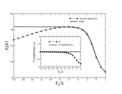
Figure 1: Density of states at the chemical potential $\mu$ as function of $E_{f}$, for $U\rightarrow\infty$ and $T=0.001\Delta$; we impose the satisfaction of the completeness relation. The $\rho_{f}\left(\mu\right)$ in FSR was calculated with Eq. (51).

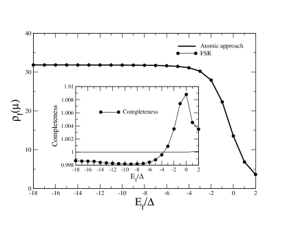
Figure 2: Density of states at the chemical potential $\mu$ as a function of $E_{f}$ for $U\rightarrow\infty$ and $T=0.001\Delta$. The $\rho_{f}\left(\mu\right)$ in FSR was calculated with Eq. (51). In this case we impose the satisfaction of Friedel’sum rule.

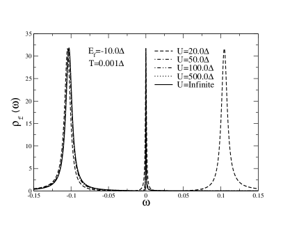
Figure 3: Density of states for $T=0.001\Delta$, $E_{f}=-10.0\Delta$ and several $U$ values: $U=20.0\Delta$, $U=50.0\Delta$, $U=100.0\Delta$, $U=500.0\Delta$ and $U=\infty$.

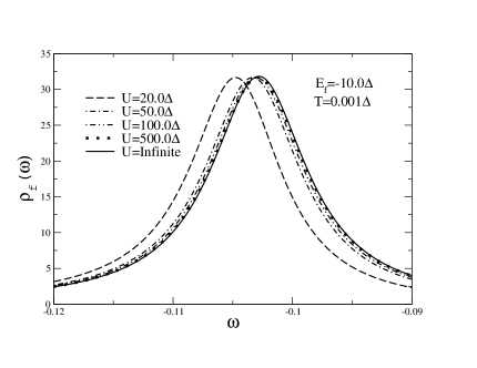
Figure 4: Detail of the lower band in the density of states of the Fig. 3.

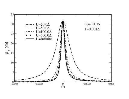
Figure 5: Detail of the Kondo peak in the density of states of the Fig. 3.

In all the figures of the paper we employ $\Delta$ units, with $\Delta=\pi V^{2}/2D=0.01$, with $D=1.0$.

In Fig. 1 we calculate the density of states at the chemical potential $\mu$ as a function of $E_{f}$, for $U\rightarrow\infty$ and $T=0.001\Delta$. In this case we impose the satisfaction of the completeness and the figure shows that in the extreme Kondo region $n_{f}\simeq 1$, there is a considerable departure of the $\rho_{f}\left(\mu\right)$ that satisfies the Friedel sum rule; in the inset of that figure we show the evolution of the occupation $n_{f}$ toward the Kondo limit and that the completeness is satisfied.

In Fig. 2 we impose the satisfaction of Friedel’sum rule. According to that figure the $f$ density of states at the chemical potential $\mu$, satisfies the FSR. In the inset of this figure we show that the completeness is lost but in the Kondo region the departure from completeness is very low; the error is less than the $1\%$, which justifies the use of FSR to determine $\varepsilon_{0}$. We shall then employ this criteria both for $U\rightarrow\infty$ and for finite $U$, because the temperatures involved in this effect are generally very low.

Next we study the evolution of the Kondo peak for finite $U$ when the correlation energy $U$ increases toward $U\rightarrow\infty$. In Fig. 3 we plot the density of states corresponding the evolution of the Kondo peak for $T=0.001\Delta$, $E_{f}=-10.0\Delta$ and several $U$ values: $U=20.0\Delta$, $U=50.0\Delta$, $U=100.0\Delta$, $U=500.0\Delta$ and $U=\infty$. We show the upper band only for $U=20.0\Delta$. In Fig. 4 we plot in detail the resonant band located around $E_{f}$: the curve with $U=500.0\Delta$ is practically coincident with the one with $U\rightarrow\infty$. In Fig. 5 we plot in detail the Kondo peak for the same values, and again the plot with $U=500.0\Delta$ practically coincides with the one for $U\rightarrow\infty$.

VI The emergence of the Kondo peak

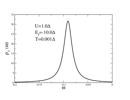
Figure 6: Density of states $\rho_{f}(\omega)$ for $U=1.0\Delta$, $E_{f}=-10.0\Delta$ and $T=0.001\Delta$.

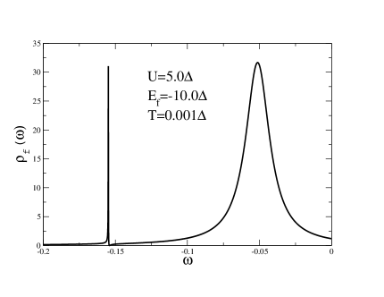
Figure 7: Density of states $\rho_{f}(\omega)$ for $U=5.0\Delta$, $E_{f}=-10.0\Delta$ and $T=0.001\Delta$.

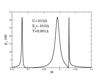
Figure 8: Density of states $\rho_{f}(\omega)$ for $U=10.0\Delta$, $E_{f}=-10.0\Delta$ and $T=0.001\Delta$.

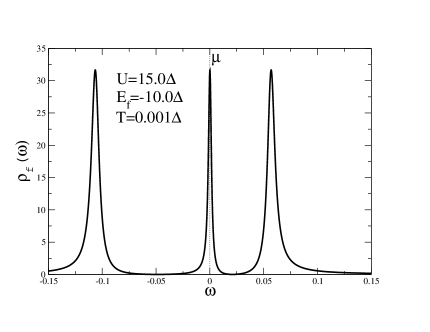
Figure 9: Density of states $\rho_{f}(\omega)$ for $U=15.0\Delta$, $E_{f}=-10.0\Delta$ and $T=0.001\Delta$.

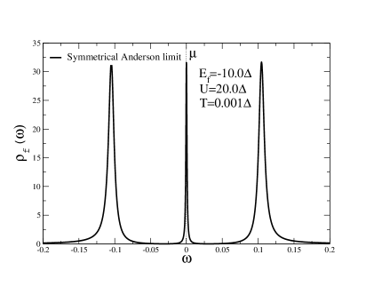
Figure 10: Density of states for $T=0.001\Delta$ , $U=20\Delta$ and $E_{f}=-10.0\Delta$. This parameter set corresponds to the symmetric case of the model and the total localized occupation number is exactly the unity $n_{f}=1.0$

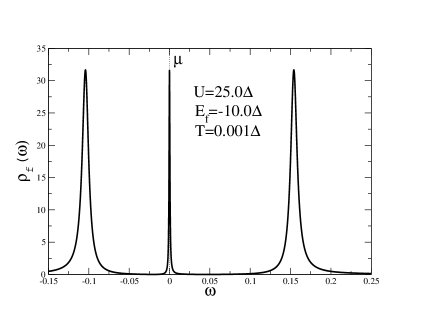
Figure 11: Density of states $\rho_{f}(\omega)$ for $U=25.0\Delta$, $E_{f}=-10.0\Delta$ and $T=0.001\Delta$.

In the set of Figs. (6-11) we show the evolution of the $f$ density of states as a function of the Coulomb repulsion $U$. We begin with the uncorrelated limit of the finite $U$ SIAM (weak coupling limit), and we consider $U=1.0\Delta$, $U=5.0\Delta$, $U=10.0\Delta$, $U=15.0\Delta$, $U=20.0\Delta$ (this value corresponds to symmetric case) and $U=25.0\Delta$.

We observe that in the Figs. (6-8), where the correlation is weak, the three peak structure characteristic of the SIAM starts to appear, but in this region the Kondo peak is not yet formed. However, for $U\simeq 15.0\Delta$ we are already in the Kondo regime for finite $U$, as shown in Fig. 9, where the Kondo peak is well defined. The Fig. 10 for $U=20.0\Delta$ corresponds to the symmetrical limit of the Anderson model, in which the total occupation number is exactly $n_{f}=1.0$. It is interesting to observe that in this case the atomic approach is able to reproduce the correct symmetry of the density of states. Finally in Fig. 11, for $U=25.0\Delta$ the Kondo peak continues pinned to the chemical potential.

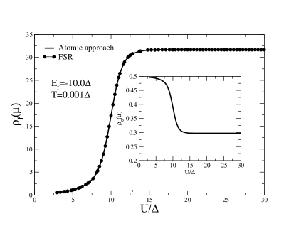
Figure 12: Density of states $\rho_{f}(\mu)$ at the chemical potential $\mu$ as function of the correlation $U$ for $E_{f}=-10.0\Delta$ and $T=0.001\Delta$, for the atomic method and for the Friedel sum rule (FSR). The FSR is represented by points over the curve. In the inset we represent the density $\rho_{c}(\mu)$ of conduction electron states at the chemical potential $\mu$, as a function of the correlation $U$.

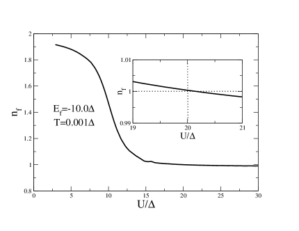
Figure 13: The total localized occupation number $n_{f}$ as a function of the correlation $U$ in $\Delta$ units. In the inset we represent the limit where the $f$ occupation number becomes exactly $n_{f}=1.0$. This point corresponds to the symmetrical limit of the Anderson hamiltonian.

In Fig. 12 we present the $f$ density of the states at the chemical potential $\mu$. At the uncorrelated side ($U<15.0\Delta$), the density of states at the chemical potential is small, but increases as the value of the correlation $U$ increases. For ($U>15.0\Delta$) we attain the Kondo regime, where the occupation number $n_{f}\simeq 1$ and the Friedel sum rule produces ($\rho_{f}(\mu)=1/\pi\Delta$) Costi86 . In the inset of the figure we present the density of states of conduction electrons $c$ at the chemical potential $\mu$, showing a loss of conduction electron states that migrate to the localized band, screening the impurity and generating the Kondo effect.

In Fig. 13 we present the total localized occupation number $n_{f}=\sum_{\sigma}n_{f,\sigma}$ as a function of the correlation $U$ in $\Delta$ units. At the non correlated side ($U<15.0\Delta$), the $f$ occupation number assume values between $n_{f}=1.0-2.0$. As the correlation $U$ increases, at around $U\simeq 15.0\Delta$, the system attains the Kondo regime and the $n_{f}$ assume values close to the $1.0$ as is expected to the Kondo limit of the model. In the inset we represent the limit where the $f$ occupation number becomes exactly $n_{f}=1.0$. This point corresponds to the symmetrical limit of the Anderson Hamiltonian.

VII The different regimes of the model

In the set of Figs. (14-19) we fix the correlation energy value in $U=20.0\Delta$ and we vary the localized level $E_{f}$ in order to describe the different regimes of the model: $E_{f}=5.0\Delta$ (empty-dot regime); $E_{f}=0.0\Delta$ (intermediate valence (IV) regime); $E_{f}=-5.0\Delta$ and $E_{f}=-15.0\Delta$ (Kondo regime), $E_{f}=-20.0\Delta$ (crossover from the Kondo to the magnetic regime) and $E_{f}=-25.0\Delta$ (magnetic regime).

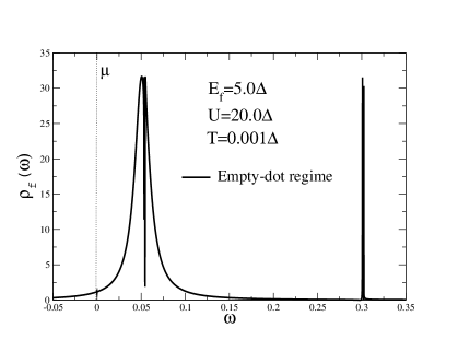
Figure 14: Density of states for $T=0.001\Delta$ , $U=20\Delta$ and $E_{f}=5.0\Delta$. This parameter set corresponds to the empty dot regime.

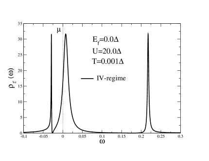
Figure 15: Density of states for $T=0.001\Delta$ , $U=20\Delta$ and $E_{f}=0.0\Delta$. This parameter set corresponds to the intermediate valence regime (IV).

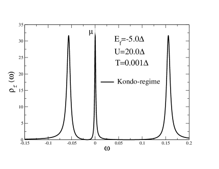
Figure 16: Density of states for $T=0.001\Delta$ , $U=20\Delta$ and $E_{f}=-5.0\Delta$. This parameter set corresponds to the beginning of the Kondo regime.

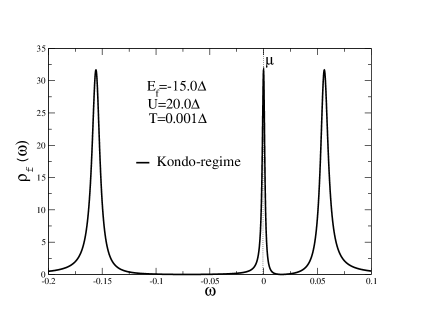
Figure 17: Density of states for $T=0.001\Delta$ , $U=20\Delta$ and $E_{f}=-15.0\Delta$. This parameter set corresponds to the ending of the Kondo regime.

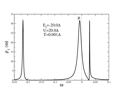
Figure 18: Density of states for $T=0.001\Delta$ , $U=20\Delta$ and $E_{f}=-20\Delta$. This region is dominated by the double occupation band and the $f$ occupation number is greater than one and corresponds to the crossover from the Kondo to the magnetic region.

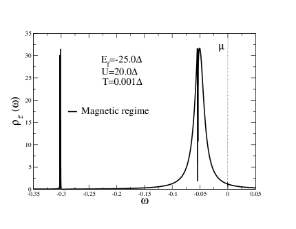
Figure 19: Density of states for $T=0.001\Delta$ , $U=20\Delta$ and $E_{f}=-25.0\Delta$. This limit is completelly dominated by the double occupation band and the $f$ occupation number is close to $2.0$ and corresponds the region where $E_{f}-U<0$.

In Fig. 14 we represent the empty dot regime. We have only a tail of the density of states below the chemical potential $\mu$ and the total occupation number is very low and is given by $n_{f}\simeq 0.12$.

In Fig. 15 we represent a typical intermediate valence situation. In this case the density of states already exhibit the three peak structures characteristic of the Kondo regime, but the Kondo peak is not yet formed; there is a large structure at the chemical potential $\mu$, that generates a strong charge fluctuation. The total occupation number is characteristic of the intermediate valence regime; $n_{f}\simeq 0.50$.

In Fig. 16 we represent the beginning of the Kondo regime for $E_{f}\simeq-5.0\Delta$ and $n_{f}\simeq 0.96$; the system remain in this regime until $E_{f}\simeq-0.15\Delta$ and $n_{f}\simeq 1.04$ as indicated in Fig. 17. In this region, the Kondo peak is well defined and is pinned at the chemical potential $\mu$, and in Fig. 22 we present a resume of all regimes. The interesting point that should be stressed here, is that the Kondo limit, where the localized occupation number is exactly equal the unity ($n_{f}=1.0$), is attained in the symmetrical limit of the Anderson model as indicated in Fig. 10.

For $E_{f}<-15.0\Delta$ the influence of the double occupation band over the Kondo effect increases more and the Kondo peak enlarges its width as indicated in the Fig. 18. In this figure $E_{f}\approx U$ and $n_{f}\simeq 1.50$ and there is no Kondo effect. We call this region the “magnetic region” because as $E_{f}$ becomes more and more negative there is a competition between the Kondo state $|11>$ and the two magnetic states $|14>$,$|15>$ of the atomic solution of the SIAM. We will discuss this point in more details in Figs. 20-22.

Finally in Fig. 19 we represent the limit where $(U+E_{f})<<0$; in this particular case the double occupation state is almost completely full and $n_{f}\simeq 1.88$.

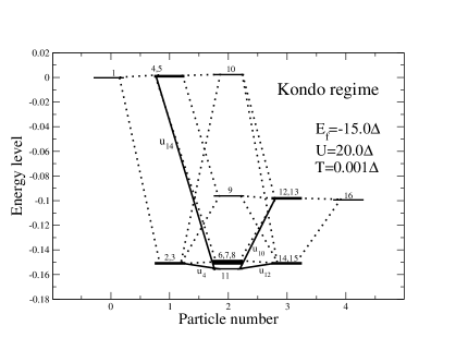
Figure 20: The sixteen energy levels $E_{n,r}$ (in units of $\Delta$) of the AAS, obtained in Appendix A (cf. Table III), as a function of the particle number for typical parameters of the Kondo regime: $U=20\Delta$, $E_{f}=-15.0\Delta$ and $T=0.001\Delta$.

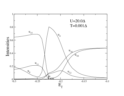
Figure 21: Intensities of the residues associating to the transition “Kondo-magnetic” as a function of $E_{f}$ (in units of $\Delta$), corresponding to $U=20\Delta$, and $T=0.001\Delta$.

It is now convenient to study in more detail the crossover region from the Kondo to the magnetic regime. In Fig. 20 we represent the sixteen energy levels $E_{n,r}\equiv E_{j}$ ($j=1,...,16)$ of the AAS (cf. Table III) as a function of the particle number, for the parameters corresponding to the ending of the Kondo regime as indicated in the Fig. 17: $U=20\Delta$, $E_{f}=-15.0\Delta$ and $T=0.001\Delta$. The lines joining them are associated to the corresponding poles $u_{i}$ (cf. Table IV) of the atomic GF in Eq. (60)  that are given in Eqs. (63-71)

When $E_{f}<0.15$ the double occupation states become available to the system and there is a competition between the singlet that originates the Kondo effect represented by the state $|11>$ in Fig. 20 and a magnetic state represented in the same figure by the two degenerate states $|14>$,$|15>$.

This point deserves a more detailed study. To do so we consider Fig. 21: at $E_{f}\simeq-22.0\Delta$ there is a change of ground state from the two-particle Kondo singlet $|11>$ to a three particle magnetic doublet $(|14>,|15>)$ and we call this point $P_{KM}$ (“Kondo-magnetic” transition). In that figure we present the transitions $u_{4},u_{12},u_{10},$ and $u_{14}$ connected to the singlet $|11>$, and their intensities are important in the Kondo region but they decrease strongly when $E_{f}$ becomes closer to the point $P_{KM}$. For values of $E_{f}<P_{KM}$ the transitions $u_{4}$,$u_{11}$ and $u_{15}$ associated to the magnetic state grow up. This region becomes relevant when the $RKKY$ interaction is present, like in the problem of several interacting impurities or in the lattice case. This interaction is associated to the magnetic transitions in the heavy fermion Kondo problem, in which case this transition is generally antiferromagnetic.

One interesting problem in which the above discussion applies is the double quantum dots problem (DQD), which has been recently proposed as a possible realization of the spin quantum computer Koppens06 . It constitutes the minimal system for studying a lattice of magnetic impurities in a tunable environment. In this system the competition between the Kondo effect and the RKKY interaction lead to a second-order quantum phase transition (QPT) but if the electrons can tunnel between impurities this QPT is replaced by a crossover Jones88 .

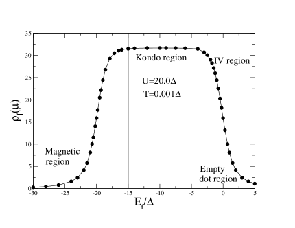
Figure 22: Density of states at the chemical potential $\mu$ vs. $E_{f}$ for $T=0.001\Delta$ , $U=20.0\Delta$.

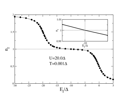
Figure 23: The total localized occupation number $n_{f}$ as a function of the correlation $E_{f}$. In the inset we represent the limit where the $f$ occupation number becomes exactly $n_{f}=1.0$. This point corresponds to the symmetrical limit of the Anderson Hamiltonian.

In Fig. 22 we show the density of states at the chemical potential $\mu$ vs. $E_{f}$ for $T=0.001\Delta$, $U=20\Delta$. The two vertical lines separate three main regions: intermediate valence to Kondo region and the Kondo region to the magnetic region. From this result, it is clear that in the case of finite $U$ the Kondo effect only exists in a limited parameter region of the SIAM. Fig. 23 shows that the Kondo behavior manifests itself when the total $f$ occupation number $n_{f}=\sum_{\sigma}n_{f,\sigma}$ assume values close to one $n_{f}=1.0$; according to the inset of the figure, this value of $n_{f}$ corresponds to the symmetrical limit of the SIAM as represented in Fig. 10.

VIII Conductance of a side-coupled quantum dot for the finite $U$ case

In this Section we apply the atomic method for finite energy correlation $U$, to study the electronic transport through a quantum wire (QW) with a side-coupled quantum dot (QD) QDnosso . The quantum dot can be occupied from zero to two electrons as a function of the chemical potential $\mu$. This system has been already studied for $U\rightarrow\infty$ when the double occupation is forbidden, Kang2001 ; QDnosso . The finite $U$ case is much more realistic, and produces interesting results Seridonio09 for the conductance that should be compared with recent experimental data Kobayashy2004 ; Masahiro05 ; Fuhrer06 .

In Fig. 24 we present a pictorial view of the quantum dot, side-coupled to a ballistic channel.

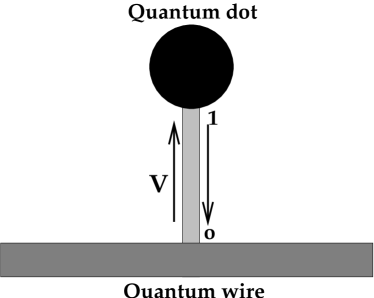
Figure 24: Pictorial view of a quantum dot side-coupled to a conduction channel.

Electron transport is coherent at low temperature and bias voltage, and a linear-response conductance is given by the Landauer-type formula Kang2001

$$G=\frac{2e^{2}}{\hbar}\int\left(-\frac{\partial n_{f}}{\partial\omega}\right)S(\omega)d\omega,$$ (53)

where $n_{F}$ is the Fermi function and $S(\omega)$ is the transmission probability of an electron with energy $\hbar\omega$. This probability is given by

$$S(\omega)=\Gamma^{2}\mid G_{00}^{\sigma}\mid^{2},$$ (54)

where $\Gamma$ corresponds to the coupling strength of the site $0$ to the wire. $G_{00}^{\sigma}$ can be calculated by the Dyson equation, where $\tilde{V}=|0\left\rangle V\right\langle 1|+|1\left\rangle V\right\langle 0|$ is the hybridization. The dressed Green’s functions at the site 0 can be written in terms of the undressed localized Green’s functions $g_{11}$ at the QD and of the undressed Green’s functions $g_{00}$ of the conduction electrons:

$$G_{00}^{\sigma}=g_{00}^{\sigma}+g_{00}^{\sigma}VG_{10}^{\sigma}+g_{01}^{\sigma}VG_{00}^{\sigma},$$ (55)

$$G_{10}^{\sigma}=g_{10}^{\sigma}+g_{10}^{\sigma}VG_{10}^{\sigma}+g_{11}^{\sigma}VG_{00}^{\sigma}.$$ (56)

Solving this system of equations, and taking into account that the non-diagonal bare conduction Green’s functions vanish: $g^{\sigma}_{10}=0$ and $g^{\sigma}_{01}=0$, we can write

$$G_{00}^{\sigma}=\frac{g_{00}^{\sigma}}{(1+g_{00}^{\sigma}V^{2}g_{11}^{\sigma})},$$ (57)

where

$$g_{00}^{\sigma}=\left(\frac{-1}{2D}\right)\ln\left(\frac{z+D+\mu}{z-D+\mu}\right)\hskip 11.38092pt;\hskip 11.38092ptg_{11}^{\sigma}=M_{\uparrow}^{at}(z),$$ (58)

and $M_{\uparrow}^{at}(z)$ is obtained employing the atomic approach Green’s functions given by Eq. (37)

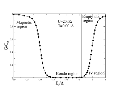
Figure 25: Conductance of the side-coupled quantum dot for $U=20.0\Delta$ and $T=0.001\Delta$.

In Fig. 25 we calculate the conductance corresponding to the parameters employed in Sec. VI. We show the conductance as a function of $E_{f}$ for $U=20\Delta$ and at temperature $T=0.001\Delta$. We can observe four important regions indicated in the graph. The first is the empty-dot region. In this situation, the value of the localized level $E_{f}$ is positive and is located above the chemical potential $\mu$; the localized occupation number goes to zero $(n_{f}\longrightarrow 0)$ and the conductance goes to one $(G/G_{0}\longrightarrow 1)$. In this situation there is practically no destructive interference between the dot and the wire.

The next regime is the intermediate valence, which is indicated in the graph by “IV region”, and the localized level $E_{f}$ is located around the chemical potential $\mu=0$. In this region the value of the $f$ occupation number varies strongly as a consequence of the charge fluctuation, the quantum interference effects start to increase and the Kondo peak appears when $n_{f}\rightarrow 1$.

The next region in the graph shows the effect of the Kondo regime in the side-coupled QD system. The occupation number is around one $(n_{f}\simeq 1)$ and the conductance goes to zero $(G/G_{0}\longrightarrow 0)$. The Kondo peak is formed, and there is a perfect destructive quantum interference of $\pi/2$ between the electrons that go around the wire and those that “visit” the QD and return to the wire.

In the last region the $f$ occupation is greater than one, and the double occupation dominates this regime as indicated in Figs. 18-19. This is the “magnetic” region and we can observe a competition between the Kondo effect and the magnetic state, as discussed in the text of Figs. 20-22. The occupation number goes to two $(n_{f}\longrightarrow 2)$ as the $E_{f}$ becomes more negative and the conductance goes again to one $(G/G_{0}\longrightarrow 1)$.

IX Conclusions

Employing the atomic approach, we characterized well the formation of the Kondo peak for all the parameters of the SIAM by calculating several curves of density of states, varying the value of the coulomb repulsion $U$, as well as the position of the localized impurity level $E_{f}$.

As a general conclusion we can say that we have developed a general and simple method to calculate the low temperature properties of the Anderson impurity model, and we call this method the atomic approach, because the starting point of the method is the zero conduction bandwidth limit of the Anderson impurity model. The approach is extremely simple, satisfies the Friedel sum rule by construction and is valid, at low temperatures, for all the relevant range of parameters and for all the coupling regimes of the SIAM, namely for the weak, intermediate and strong correlation regimes of the model.

The atomic approach is a good candidate to describe nanoscopic systems with correlated electrons that present Kondo effect, and it produces excellent results for the occupation numbers and for the dynamical properties. Due to its simplicity, low computational cost (the computational time consuming to obtain a density of states curve takes few seconds or less) the atomic approach could be applied to study nanoscopic correlated systems, like quantum dots.

Appendix A The atomic Green functions

$$\begin{array}[]{|l|c|c|c|}\hline\cr|m,\sigma>&E&n&S_{z}\\ \hline\cr|0,0>&0&0&0\\ \hline\cr|+,0>&\varepsilon_{f}&1&1/2\\ \hline\cr|0,\uparrow>&\varepsilon_{q}&1&1/2\\ \hline\cr|-,0>&\varepsilon_{f}&1&-1/2\\ \hline\cr|0,\downarrow>&\varepsilon_{q}&1&-1/2\\ \hline\cr|+,\uparrow>&\varepsilon_{f}+\varepsilon_{q}&2&1\\ \hline\cr|-,\downarrow>&\varepsilon_{f}+\varepsilon_{q}&2&-1\\ \hline\cr|+,\downarrow>&\varepsilon_{f}+\varepsilon_{q}&2&0\\ \hline\cr|-,\uparrow>&\varepsilon_{f}+\varepsilon_{q}&2&0\\ \hline\cr|0,\uparrow\downarrow>&2\varepsilon_{q}&2&0\\ \hline\cr|d,0>&2\varepsilon_{f}+U&2&0\\ \hline\cr|d,\uparrow>&2\varepsilon_{f}+\varepsilon_{q}+U&3&1/2\\ \hline\cr|+,\uparrow\downarrow>&\varepsilon_{f}+2\varepsilon_{q}&3&1/2\\ \hline\cr|d,\downarrow>&2\varepsilon_{f}+\varepsilon_{q}+U&3&-1/2\\ \hline\cr|-,\uparrow\downarrow>&\varepsilon_{f}+2\varepsilon_{q}&3&-1/2\\ \hline\cr|d,\uparrow\downarrow>&2\varepsilon_{f}+2\varepsilon_{q}+U&4&0\\ \hline\cr\end{array}$$

Table 2: States of the Anderson impurity in the limit $2D=V=0$. The columns indicates the states $|n,\sigma>$, the energies $E_{o}$, the number of electrons $n$ and the spin component $S_{z}$.

In this Appendix we present the details of the calculation of the exact Green’s function of the Anderson impurity model in the limit of zero conduction bandwidth. In this limit all the hoping contributions are eliminated from the Hamiltonian, because we also take $V_{f,\mathbf{k},\sigma}=V$ in Eqs. (11-12), i.e.: a local hybridization. Transforming the conduction electrons to the Wannier representation we then have an independent system at each site of the crystal. In this limit there is an isolated metal atom at each site, one of them being the Anderson impurity, and the system Hamiltonian can be diagonalized exactly. In the Anderson Hamiltonian, there are four possible occupations $(0,\uparrow,\downarrow,\uparrow\downarrow)$ of the conduction electrons at any site, and at the impurity there are also four possible occupations of the local $f$ electrons: $(0,+\frac{1}{2},-\frac{1}{2},d)$. At the impurity site we then have a Fock space with sixteen states characterized by $|m,\sigma>$ as shown in Table 2, and the hybridization mixes states with equal particle number and with the same spin component $z$. We should then diagonalize a $16$x$16$ matrix which presents a block structure that simplifies the calculation, because the greater block is $3$x$3$ and we employ Cardano’s formula to solve the associated third degree algebraic equation. The results of this calculation are presented in Table 3.

$$\begin{array}[]{|l|l|c|c|}\hline\cr Eigenstates\hskip 8.5359pt|j>\equiv|n,r>&Eigenvalues\text{ }E_{j}\equiv E_{n,r}&n&S_{z}\\ \hline\cr|1>\equiv|0,1>=|0,0\rangle&E_{1}\equiv E_{0,1}=0&0&0\\ \hline\cr|2\rangle\equiv|1,1>=\cos\phi|+,0\rangle-\sin\phi|0,\uparrow\rangle&E_{2}\equiv E_{1,1}=\frac{1}{2}(\varepsilon_{f}+\varepsilon_{q}-\Delta)&1&+\frac{1}{2}\\ \hline\cr|3\rangle\equiv|1,2>=\cos\phi|-,0\rangle-\sin\phi|0,\downarrow\rangle&E_{3}\equiv E_{1,2}=E_{2}&1&-\frac{1}{2}\\ \hline\cr|4\rangle\equiv|1,3>=\sin\phi|+,0\rangle+\cos\phi|0,\uparrow\rangle&E_{4}\equiv E_{1,3}=\frac{1}{2}(\varepsilon_{f}+\varepsilon_{q}+\Delta)&1&+\frac{1}{2}\\ \hline\cr|5\rangle\equiv|1,4>=\sin\phi|-,0\rangle+\cos\phi|0,\downarrow\rangle&E_{5}\equiv E_{1,4}=E_{4}&1&-\frac{1}{2}\\ \hline\cr|6\rangle\equiv|2,1>=|+,\uparrow\rangle&E_{6}\equiv E_{2,1}=\varepsilon_{f}+\varepsilon_{q}&2&1\\ \hline\cr|7\rangle\equiv|2,2>=|-,\downarrow\rangle&E_{7}\equiv E_{2,2}=E_{6}&2&-1\\ \hline\cr|8\rangle\equiv|2,3>=1/\sqrt{2}(|+,\downarrow\rangle+|-,\uparrow\rangle)&E_{8}\equiv E_{2,3}=E_{7}&2&0\\ \hline\cr|9\rangle\equiv|2,4>=a_{9}[|+,\downarrow\rangle-|-,\uparrow\rangle]+b_{9}|d,0\rangle+c_{9}|0,\uparrow\downarrow\rangle&E_{9}\equiv E_{2,4}=2\sqrt{-Q}\cos(\frac{\theta_{1}}{3})&2&0\\ \hline\cr|10\rangle\equiv|2,5>=a_{10}[|+,\downarrow\rangle-|-,\uparrow\rangle]+b_{10}|d,0\rangle+c_{10}|0,\uparrow\downarrow\rangle&E_{10}\equiv E_{2,5}=2\sqrt{-Q}\cos(\frac{\theta_{1}+2\pi}{3})&2&0\\ \hline\cr|11\rangle\equiv|2,6>=a_{11}[|+,\downarrow\rangle-|-,\uparrow\rangle]+b_{11}|d,0\rangle+c_{11}|0,\uparrow\downarrow\rangle&E_{11}\equiv E_{2,6}=2\sqrt{-Q}\cos(\frac{\theta_{1}+4\pi}{3})&2&0\\ \hline\cr|12\rangle\equiv|3,1>=\sin(\theta)|d,\uparrow\rangle+\cos(\theta)|+,\uparrow\downarrow\rangle&E_{12}\equiv E_{3,1}=\frac{1}{2}(3\varepsilon_{f}+3\varepsilon_{q}+U+\Delta^{\prime})&3&+\frac{1}{2}\\ \hline\cr|13\rangle\equiv|3,2>=\sin(\theta)|d,\downarrow\rangle+\cos(\theta)|-,\uparrow\downarrow\rangle&E_{13}\equiv E_{3,2}=E_{12}&3&-\frac{1}{2}\\ \hline\cr|14\rangle\equiv|3,3>=-\cos(\theta)|d,\uparrow\rangle+\sin(\theta)|+,\uparrow\downarrow\rangle&E_{14}\equiv E_{3,3}=\frac{1}{2}(3\varepsilon_{f}+3\varepsilon_{q}+U-\Delta^{\prime})&3&+\frac{1}{2}\\ \hline\cr|15\rangle\equiv|3,4>=-\cos(\theta)|d,\downarrow\rangle+\sin(\theta)|-,\uparrow\downarrow\rangle&E_{15}\equiv E_{3,4}=E_{14}&3&-\frac{1}{2}\\ \hline\cr|16\rangle\equiv|4,1>=|d,\uparrow\downarrow\rangle&E_{16}\equiv E_{4,1}=2\varepsilon_{f}+2\varepsilon_{q}+U&4&0\\ \hline\cr\end{array}$$

Table 3: Exact solution (AAS) of the Anderson model in the limit of local hybridization and conduction band with zero width. The sixteen eigenstates $\mid n,r\rangle$ have energies $E_{n,r}$, where $n$ is the number of electrons and $S_{z}$ is the spin component, and we abbreviate $|j>\equiv|n,r>$ and $E_{j}\equiv E_{n,r}$ $(j=1,\ldots,16)$.We use $\varepsilon_{n,r}=E_{n,r}-n\mu$, and the other parameters are given by
$\Delta=[(\varepsilon_{f}-\varepsilon_{q})^{2}+4V^{2}]^{1/2}$; $\Delta^{\prime}=[(\varepsilon_{f}+U-\varepsilon_{q})^{2}+4V^{2}]^{1/2}$;
$tg\phi=2V/(\varepsilon_{q}-\varepsilon_{f}+\Delta)$; $tg\theta=2V/(\varepsilon_{f}+U-\varepsilon_{q}-\Delta^{\prime})$;
$a_{i}=\frac{1}{\sqrt{2+4V^{2}[(E_{i}-2\varepsilon_{f}-U)^{-2}+(E_{i}-2\varepsilon_{q})^{-2}]}}$; $b_{i}=\frac{2V}{E_{i}-2\varepsilon_{f}-U}a_{i}$; $c_{i}=\frac{2V}{E_{9}-2\varepsilon_{q}}a_{i}$; $i=9,10,11$;
$\theta_{1}=\arccos\frac{R}{\sqrt{(-Q)^{3}}}$; $Q=-\frac{1}{9}[12V^{2}+(\varepsilon_{q}+\varepsilon_{f})^{2}+(2\varepsilon_{f}+U)^{2}+(2\varepsilon_{q})^{2}-(\varepsilon_{q}+\varepsilon_{f})(2\varepsilon_{f}+U)-(\varepsilon_{q}+\varepsilon_{f})(2\varepsilon_{q})-(2\varepsilon_{f}+U)(2\varepsilon_{q})]$;
$R=\frac{1}{54}\{-3[(\varepsilon_{q}+\varepsilon_{f})^{2}(2\varepsilon_{f}+U)+(\varepsilon_{q}+\varepsilon_{f})^{2}(2\varepsilon_{q})+(2\varepsilon_{f}+U)^{2}(\varepsilon_{q}+\varepsilon_{f})+(2\varepsilon_{f}+U)^{2}(2\varepsilon_{q})+(2\varepsilon_{q})^{2}(\varepsilon_{q}+\varepsilon_{f})+(2\varepsilon_{q})^{2}(2\varepsilon_{f}+U)]+12(\varepsilon_{q}+\varepsilon_{f})(2\varepsilon_{f}+U)(2\varepsilon_{q})+18V^{2}[2(\varepsilon_{q}+\varepsilon_{f})-(2\varepsilon_{f}+U)-(2\varepsilon_{q})]+2[(\varepsilon_{q}+\varepsilon_{f})^{3}+(2\varepsilon_{f}+U)^{3}+(2\varepsilon_{q})^{3}]\}$.

To obtain the localized atomic Green’s functions of the impurity in the zero width limit, we use Zubarev’s Zubarev60 equation

$$\mathcal{G}_{\alpha\alpha^{\prime}}^{ff,at}(i\omega_{s})=-e^{\beta\Omega}\sum_{n,r,r^{\prime}}\frac{\exp(-\beta\varepsilon_{n-1,r})+\exp(-\beta\varepsilon_{n,r^{\prime}})}{i\omega_{s}+\varepsilon_{n-1,r}-\varepsilon_{n,r^{\prime}}}\times$$

$$\times\left\langle n-1,r\right|\ X_{j,\alpha}\left|n,r^{\prime}\right\rangle\left\langle n,r^{\prime}\right|\ X_{j,\alpha^{\prime}}^{\dagger}\ \left|n-1,r\right\rangle,$$ (59)

where $\Omega$ is the thermodynamical potential and the eigenvalues $E_{nj}$ and eigenvectors $|nj>$ correspond to the complete solution of the Hamiltonian. The final result is the following

$$G^{ff,at}(\omega)=e^{\beta\Omega}\sum_{i=1}^{16}\frac{m_{i}}{\omega-u_{i}},$$ (60)

where the $u_{i}$ poles of the Green’s functions are given in Table 4

$u_{1}=$	$E_{2}-E_{1}=E_{6}-E_{4}$
$u_{2}=$	$E_{5}-E_{1}=E_{6}-E_{2}$
$u_{3}=$	$E_{10}-E_{2}$
$u_{4}=$	$E_{11}-E_{2}$
$u_{5}=$	$E_{9}-E_{2}$
$u_{6}=$	$E_{10}-E_{4}$
$u_{7}=$	$E_{12}-E_{6}=E_{16}-E_{14}$
$u_{8}=$	$E_{12}-E_{9}$
$u_{9}=$	$E_{12}-E_{10}$
$u_{10}=$	$E_{12}-E_{11}$
$u_{11}=$	$E_{14}-E_{10}$
$u_{12}=$	$E_{14}-E_{11}$
$u_{13}=$	$E_{9}-E_{4}$
$u_{14}=$	$E_{11}-E_{4}$
$u_{15}=$	$E_{14}-E_{6}=E_{16}-E_{12}$
$u_{16}=$	$E_{14}-E_{9}$

Table 4: Poles of the Green’s functions, corresponding to all the possible transitions in the atomic solution.

The residues for the localized electrons are given by
$m_{1}=cos(\phi)^{2}[e^{-\beta E_{1}}+e^{-\beta E_{2}}+\frac{3}{2}e^{-\beta E_{4}}+\frac{3}{2}e^{-\beta E_{6}}]$,
$m_{2}=sin(\phi)^{2}[e^{-\beta E_{1}}+e^{-\beta E_{4}}+\frac{3}{2}e^{-\beta E_{2}}+\frac{3}{2}e^{-\beta E_{6}}]$,
$m_{3}=(e^{-\beta E_{3}}+e^{-\beta E_{10}})[(a_{10}sin(\phi))^{2}+(b_{10}cos(\phi))^{2}]$,
$m_{4}=(e^{-\beta E_{3}}+e^{-\beta E_{11}})[(a_{11}sin(\phi))^{2}+(b_{11}cos(\phi))^{2}]$,
$m_{5}=(e^{-\beta E_{3}}+e^{-\beta E_{9}})[(a_{9}sin(\phi))^{2}+(b_{9}cos(\phi))^{2}]$,
$m_{6}=(e^{-\beta E_{4}}+e^{-\beta E_{10}})[(a_{10}cos(\phi))^{2}+(b_{10}sin(\phi))^{2}]$,
$m_{7}=sin(\theta)^{2}[\frac{3}{2}(e^{-\beta E_{8}}+e^{-\beta E_{12}})+(e^{-\beta E_{15}}+e^{-\beta E_{16}})]$,
$m_{8}=(e^{-\beta E_{9}}+e^{-\beta E_{12}})[(c_{9}cos(\theta))^{2}+(a_{9}sin(\theta))^{2}]$,
$m_{9}=(e^{-\beta E_{10}}+e^{-\beta E_{12}})[(c_{10}cos(\theta))^{2}+(a_{10}sin(\theta))^{2}]$,
$m_{10}=(e^{-\beta E_{11}}+e^{-\beta E_{12}})[(c_{11}cos(\theta))^{2}+(a_{11}sin(\theta))^{2}]$,
$m_{11}=(e^{-\beta E_{10}}+e^{-\beta E_{14}})[(c_{10}sin(\theta))^{2}+(a_{10}cos(\theta))^{2}]$,
$m_{12}=(e^{-\beta E_{11}}+e^{-\beta E_{15}})[(c_{11}sin(\theta))^{2}+(a_{11}cos(\theta))^{2}]$,
$m_{13}=(e^{-\beta E_{5}}+e^{-\beta E_{9}})[(a_{9}cos(\phi))^{2}+(b_{9}sin(\phi))^{2}]$,
$m_{14}=(e^{-\beta E_{5}}+e^{-\beta E_{11}})[(a_{11}cos(\phi))^{2}+(b_{11}sin(\phi))^{2}]$,
$m_{15}=cos(\theta))^{2}\left[\frac{3}{2}(e^{-\beta E_{8}}+e^{-\beta E_{14}})+(e^{-\beta E_{13}}+e^{-\beta E_{16}})\right]$,
$m_{16}=(e^{-\beta E_{9}}+e^{-\beta E_{15}})[(a_{9}cos(\theta))^{2}+(c_{9}sin(\theta))^{2}]$,
and for the electrons $c$ we have

$$\mathcal{G}_{\alpha\alpha^{\prime}}^{cc,at}(i\omega_{s})=-e^{\beta\Omega}\sum_{n,r,r^{\prime}}\frac{\exp(-\beta\varepsilon_{n-1,r})+\exp(-\beta\varepsilon_{n,r^{\prime}})}{i\omega_{s}+\varepsilon_{n-1,r}-\varepsilon_{n,r^{\prime}}}\times$$

$$\times\left\langle n-1,r\right|\ c_{\vec{k},\alpha}\left|n,r^{\prime}\right\rangle\left\langle n,r^{\prime}\right|\ c_{\vec{k},\alpha^{\prime}}^{\dagger}\ \left|n-1,r\right\rangle,$$ (61)

$$G^{cc,at}(\omega)=e^{\beta\Omega}\sum_{i=1}^{16}\frac{n_{i}}{\omega-u_{i}},$$ (62)

and the residues for the conduction electrons are given by

$n_{1}=sin(\phi)^{2}[e^{-\beta E_{1}}+e^{-\beta E_{2}}+\frac{3}{2}e^{-\beta E_{4}}+\frac{3}{2}e^{-\beta E_{8}}]$,
$n_{2}=cos(\phi)^{2}[e^{-\beta E_{1}}+e^{-\beta E_{5}}+\frac{3}{2}e^{-\beta E_{3}}+\frac{3}{2}e^{-\beta E_{8}}]$,
$n_{3}=(e^{-\beta E_{2}}+e^{-\beta E_{10}})[(a_{10}cos(\phi))^{2}+(c_{10}sin(\phi))^{2}]$,
$n_{4}=(e^{-\beta E_{2}}+e^{-\beta E_{11}})[(a_{11}cos(\phi))^{2}+(c_{11}sin(\phi))^{2}]$,
$n_{5}=(e^{-\beta E_{2}}+e^{-\beta E_{9}})[(a_{9}cos(\phi))^{2}+(c_{9}sin(\phi))^{2}]$,
$n_{6}=(e^{-\beta E_{4}}+e^{-\beta E_{10}})[(a_{10}sin(\phi))^{2}+(c_{10}cos(\phi))^{2}]$,
$n_{7}=cos(\theta)^{2}[e^{-\beta E_{16}}+e^{-\beta E_{14}}+\frac{3}{2}e^{-\beta E_{8}}+\frac{3}{2}e^{-\beta E_{13}}]$,
$n_{8}=(e^{-\beta E_{9}}+e^{-\beta E_{12}})[(a_{9}cos(\theta))^{2}+(b_{9}sin(\theta))^{2}]$,
$n_{9}=(e^{-\beta E_{10}}+e^{-\beta E_{12}})[(a_{10}cos(\theta))^{2}+(b_{10}sin(\theta))^{2}]$,
$n_{10}=(e^{-\beta E_{11}}+e^{-\beta E_{12}})[(a_{11}cos(\theta))^{2}+(b_{11}sin(\theta))^{2}]$,
$n_{11}=(e^{-\beta E_{10}}+e^{-\beta E_{14}})[(a_{10}sin(\theta))^{2}+(b_{10}cos(\theta))^{2}]$,
$n_{12}=(e^{-\beta E_{11}}+e^{-\beta E_{14}})[(b_{11}cos(\theta))^{2}+(a_{11}sin(\theta))^{2}]$.
$n_{13}=(e^{-\beta E_{4}}+e^{-\beta E_{9}})[(c_{9}cos(\phi))^{2}+(a_{9}sin(\phi))^{2}]$,
$n_{14}=(e^{-\beta E_{4}}+e^{-\beta E_{11}})[(c_{11}cos(\phi))^{2}+(a_{11}sin(\phi))^{2}]$,
$n_{15}=sin(\theta)^{2}[e^{-\beta E_{12}}+e^{-\beta E_{16}}+\frac{3}{2}e^{-\beta E_{14}}+\frac{3}{2}e^{-\beta E_{6}}]$,
$n_{16}=(e^{-\beta E_{9}}+e^{-\beta E_{14}})[(b_{9}cos(\theta))^{2}+(a_{9}sin(\theta))^{2}]$,

Finally following the same definition for the cumulants in Eq. (23) we can write all the atomic Green’s functions employed in the calculation of the atomic approach.

$$\mathbf{G}_{\uparrow}^{ff,at}=\begin{pmatrix}g_{11}&g_{13}\\ g_{31}&g_{33}\end{pmatrix}\hskip 20.0pt\mathrm{;\hskip 20.0pt}\mathbf{G}_{\downarrow}^{ff,at}=\begin{pmatrix}g_{22}&g_{24}\\ g_{42}&g_{44}\end{pmatrix},$$ (63)

$$g_{11}=e^{-\beta\Omega}\biggl{\{}\left[sin^{2}\phi\left(\frac{e^{-\beta E_{1}}+e^{-\beta E_{4}}}{i\omega+E_{1}-E_{4}}+\frac{3}{2}\frac{e^{-\beta E_{2}}+e^{-\beta E_{6}}}{i\omega+E_{2}-E_{6}}\right)\right.\newline$$

$$\left.+\cos^{2}\phi\left(\frac{e^{-\beta E_{1}}+e^{-\beta E_{2}}}{i\omega+E_{1}-E_{2}}+\frac{3}{2}\frac{e^{-\beta E_{4}}+e^{-\beta E_{6}}}{i\omega+E_{4}-E_{6}}\right)\right]\newline$$

$$+\sum_{i=9}^{11}\left[\frac{e^{-\beta E_{3}}+e^{-\beta E_{i}}}{i\omega+E_{3}-E_{i}}(a_{i}\sin\phi)^{2}+\frac{e^{-\beta E_{5}}+e^{-\beta E_{i}}}{i\omega+E_{5}-E_{i}}(a_{i}\cos\phi)^{2}\right.\newline \newline$$

$$\left.+\frac{e^{-\beta E_{i}}+e^{-\beta E_{14}}}{i\omega+E_{i}-E_{14}}(c_{i}\sin\theta)^{2}+\frac{e^{-\beta E_{i}}+e^{-\beta E_{12}}}{i\omega+E_{i}-E_{12}}(c_{i}\cos\theta)^{2}\right]\biggr{\}},$$ (64)

$$g_{33} = e^{-\beta\Omega}\biggl{\{}\left[sin^{2}\theta\left(\frac{e^{-\beta E_{15}}+e^{-\beta E_{16}}}{i\omega+E_{15}-E_{16}}+\frac{3}{2}\frac{e^{-\beta E_{8}}+e^{-\beta E_{12}}}{i\omega+E_{8}-E_{12}}\right)\right.\newline$$ (65)

$$\left.+\cos^{2}\theta\left(\frac{e^{-\beta E_{13}}+e^{-\beta E_{16}}}{i\omega+E_{13}-E_{16}}+\frac{3}{2}\frac{e^{-\beta E_{8}}+e^{-\beta E_{14}}}{i\omega+E_{8}-E_{14}}\right)\right]$$

$$+\sum_{i=9}^{11}\left[\frac{e^{-\beta E_{4}}+e^{-\beta E_{i}}}{i\omega+E_{4}-E_{i}}(b_{i}\sin\phi)^{2}+\frac{e^{-\beta E_{3}}+e^{-\beta E_{i}}}{i\omega+E_{3}-E_{i}}(b_{i}\cos\phi)^{2}\right.$$

$$\left.+\frac{e^{-\beta E_{i}}+e^{-\beta E_{12}}}{i\omega+E_{i}-E_{12}}(a_{i}\sin\theta)^{2}+\frac{e^{-\beta E_{i}}+e^{-\beta E_{14}}}{i\omega+E_{i}-E_{14}}(a_{i}\cos\theta)^{2}\right]\biggr{\}},$$

$$g_{13} = e^{-\beta\Omega}\sum_{i=9}^{11}\biggl{\{}\left[\frac{e^{-\beta E_{5}}+e^{-\beta E_{i}}}{i\omega+E_{5}-E_{i}}-\frac{e^{-\beta E_{3}}+e^{-\beta E_{i}}}{i\omega+E_{3}-E_{i}}\right](a_{i}b_{i}\sin\phi\cos\phi)$$ (66)

$$+\left[\frac{e^{-\beta E_{i}}+e^{-\beta E_{14}}}{i\omega+E_{i}-E_{14}}-\frac{e^{-\beta E_{i}}+e^{-\beta E_{12}}}{i\omega+E_{i}-E_{12}}\right](a_{i}c_{i}\sin\theta\cos\theta)\biggr{\}}$$

$$g_{31}=g_{13},$$ (67)

$$g_{22} = e^{-\beta\Omega}\biggl{\{}\left[sin^{2}\phi\left(\frac{e^{-\beta E_{1}}+e^{-\beta E_{5}}}{i\omega+E_{1}-E_{5}}+\frac{3}{2}\frac{e^{-\beta E_{3}}+e^{-\beta E_{7}}}{i\omega+E_{3}-E_{7}}\right)\right.\newline$$ (68)

$$\left.+\cos^{2}\phi\left(\frac{e^{-\beta E_{1}}+e^{-\beta E_{3}}}{i\omega+E_{1}-E_{3}}+\frac{3}{2}\frac{e^{-\beta E_{5}}+e^{-\beta E_{7}}}{i\omega+E_{5}-E_{7}}\right)\right]$$

$$+\sum_{i=9}^{11}\left[\frac{e^{-\beta E_{2}}+e^{-\beta E_{i}}}{i\omega+E_{2}-E_{i}}(a_{i}\sin\phi)^{2}+\frac{e^{-\beta E_{4}}+e^{-\beta E_{i}}}{i\omega+E_{4}-E_{i}}(a_{i}\cos\phi)^{2}\right.$$

$$\left.+\frac{e^{-\beta E_{i}}+e^{-\beta E_{15}}}{i\omega+E_{i}-E_{15}}(c_{i}\sin\theta)^{2}+\frac{e^{-\beta E_{i}}+e^{-\beta E_{13}}}{i\omega+E_{i}-E_{13}}(c_{i}\cos\theta)^{2}\right]\biggr{\}},$$

$$g_{44} = e^{-\beta\Omega}\biggl{\{}\left[sin^{2}\theta\left(\frac{e^{-\beta E_{14}}+e^{-\beta E_{16}}}{i\omega+E_{14}-E_{16}}+\frac{3}{2}\frac{e^{-\beta E_{6}}+e^{-\beta E_{12}}}{i\omega+E_{6}-E_{12}}\right)\right.+$$ (69)

$$\left.+\cos^{2}\theta\left(\frac{e^{-\beta E_{12}}+e^{-\beta E_{16}}}{i\omega+E_{12}-E_{16}}+\frac{3}{2}\frac{e^{-\beta E_{6}}+e^{-\beta E_{14}}}{i\omega+E_{6}-E_{14}}\right)\right]$$

$$\sum_{i=9}^{11}\left[\frac{e^{-\beta E_{4}}+e^{-\beta E_{i}}}{i\omega+E_{4}-E_{i}}(b_{i}\sin\phi)^{2}+\frac{e^{-\beta E_{2}}+e^{-\beta E_{i}}}{i\omega+E_{2}-E_{i}}(b_{i}\cos\phi)^{2}\right.$$

$$\left.+\frac{e^{-\beta E_{i}}+e^{-\beta E_{13}}}{i\omega+E_{i}-E_{13}}(a_{i}\sin\theta)^{2}+\frac{e^{-\beta E_{i}}+e^{-\beta E_{15}}}{i\omega+E_{i}-E_{15}}(a_{i}\cos\theta)^{2}\right]\biggr{\}},$$

$$g_{24} = e^{-\beta\Omega}\sum_{i=9}^{11}\biggl{\{}\left[\frac{e^{-\beta E_{2}}+e^{-\beta E_{i}}}{i\omega+E_{2}-E_{i}}-\frac{e^{-\beta E_{4}}+e^{-\beta E_{i}}}{i\omega+E_{4}-E_{i}}\right](a_{i}b_{i}\sin\phi\cos\phi)$$ (70)

$$+\left[\frac{e^{-\beta E_{i}}+e^{-\beta E_{13}}}{i\omega+E_{i}-E_{13}}-\frac{e^{-\beta E_{i}}+e^{-\beta E_{15}}}{i\omega+E_{i}-E_{15}}\right](a_{i}c_{i}\sin\theta\cos\theta)\biggr{\}},$$

$$g_{42}=g_{24}.$$ (71)

References

• (1) M. E. Foglio, T. Lobo and M. S. Figueira, Green’s functions for the anderson model: The atomic approximation - arXiv:0903.0139v1 [cond-mat.str-el] - submitted to Reviews in Mathematical Physics.
• (2) A. M. Clogston, B. T. Mathias, M. Peter, H. J. Willians, E. Corenzwit, e R. C. Sherwood Phys. Rev. 125, 541 (1962).
• (3) J. Kondo, Progr. Theor. Phys. 2 37 (1964); J. Kondo Solid State Physics, 3 184 (1969).
• (4) Goldhaber-Gordon D et.al. Nature 391 156 (1998).
• (5) Y. Meir, P. A. Lee Phys. Rev. Lett. 70, 2601 (1993).
• (6) H. G. Luo and J. J. Ying, Phys. Rev. B, 59, 9710 (1999).
• (7) T. Lobo, M. S. Figueira, R. Franco, J. Silva-Valencia and M. E. Foglio, Physica B - Condensed Matter 398, 446 (2007).
• (8) P. Coleman, Phys. Rev. B. 29 3035 (1984).
• (9) R. Franco, M. S. Figueira and M. E. Foglio, Phys. Rev. B, 66 045112 (2002).
• (10) E. Logan, M. P. Ewastwood, and M. A. Tusch, J. Phys.: Condens. Matter 10, 2673 (1998).
• (11) Václav Janis̃ and Pavel Augustinský, Phys. Rev. B 77, 085106 (2008).
• (12) Fye and J. E. Hirsch, Phys. Rev. B 38, 433 (1988).
• (13) Georges A, Kotliar G, Krauth W and Rozenberg M J 1996 Rev. Mod. Phys. 68 13
• (14) Schollwöck U 2005 Rev. Mod. Phys. 77 259
• (15) G. Wilson, Rev. Mod. Phys. 47, 773 (1975).
• (16) A. Costi, A. C. Hewson, and V. Zlati{ae, J. Phys.: Condens. Matter 6 , 2519 (1994).
• (17) R. Bulla, A. C. Hewson, and T. Pruschke, J. Phys.: Condens. Matter 10, 8365 (1998).
• (18) T. A. Costi , J. Kroha and P. Wölfle Phys.Rev. B, 53 1850 (1996).
• (19) T. Lobo, M. S. Figueira and M. E. Foglio, Brazilian Journal of Physics, 36 397 (2006).
• (20) T. Lobo, M. S. Figueira and M. S. Ferreira, Brazilian Journal of Physics 36 401 (2006).
• (21) T. Lobo, M. S. Figueira and M. E. Foglio Nanotechnology, 17, 6016 (2006).
• (22) M. S. Figueira, M. E. Foglio and G. G. Martinez Phys. Rev. B, 50 17933 (1994).
• (23) R. Franco, M. S. Figueira and E. V. Anda, Phys. Rev. B 67 155301 (2003).
• (24) K. Kobayashi, H. Aikawa, A. Sano, S. Katsumoto and Y. Iye, Phys. Rev. B 70 035319 (2004).
• (25) M. E. Foglio and L. M. Falicov, Phys. Rev. B 20 4554 (1979).
• (26) M. E. Foglio, C. A. Balseiro and L. M. Falicov, Phys. Rev. B 20 4560 (1979).
• (27) Acirete S. da Rosa Simões, J. R. Iglesias, A. Rojo and B. R. Alascio, J. Phys. C: Solid State Phys. 21 (1988) 1941.
• (28) Canio Noce, J. Phys. C: Solid State Phys. 3 (1991) 7819; Maria Marinaro, Canio Noce and Alfonso Romano, J. Phys. C: Solid State Phys. 3 (1991) 3719.
• (29) B. Alascio, R. Allub and A. A. Aligia, Z. Phys. B, 6 37 (1979); J. Phys. C: Solid State Phys. 3 2869 (1980).
• (30) D. D. Langreth, Phys. Rev. 150 516 (1966).
• (31) K. Kang, S. Y. Cho, J. J. Kim and S. C. Shin, Phys. Rev. B 63 113304 (2001).
• (32) T. A. Costi, J. Phys. C, 19 5665 (1986).
• (33) F. H. L. Koppens, C. Buizert, K. J. Tielrooij, I. T. Vink, K. C. Nowack, T. Meunier, L. P. Kouwenhoven and L. M. K. Vandersypen, Science 442 766 (2006).
• (34) B. A. Jones, C. M. Varma, and J. W. Wilkins, Phys. Rev. Lett. 61, 125 (1988); B. A. Jones, G. Kotliar, and A. J. Millis, Phys. Rev. B 39, 3415 (1989).
• (35) A. C. Seridonio, M. Yoshida, L. N. Oliveira, Europhysics Letters, 86 67006 (2009).
• (36) Masahiro Sato, Hisashi Aikawa, Kensuke Kobayashi, Shingo Katsumoto, and Yasuhiro Iye, Phys. Rev. Lett. 95 066801 (2005).
• (37) A. Fuhrer, P. Brusheim, T. Ihn, M. Sigrist, K. Ensslin, W. Wegscheider and M. Bichler, Phys. Rev. B 73 205326 (2006).
• (38) D. N. Zubarev, Sov. Phys. Uspekhi 3 320 (1960).