A nonperturbative calculation of the electron’s magnetic moment with truncation extended to two photons

Abstract

The Pauli–Villars (PV) regularization scheme is applied to a calculation of the dressed-electron state and its anomalous magnetic moment in light-front-quantized quantum electrodynamics (QED) in Feynman gauge. The regularization is provided by heavy, negative-metric fields added to the Lagrangian. The light-front QED Hamiltonian then leads to a well-defined eigenvalue problem for the dressed-electron state expressed as a Fock-state expansion. The Fock-state wave functions satisfy coupled integral equations that come from this eigenproblem. A finite system of equations is obtained by truncation to no more than two photons and no positrons; this extends earlier work that was limited to dressing by a single photon. Numerical techniques are applied to solve the coupled system and compute the anomalous moment, for which we obtain agreement with experiment, within numerical errors, but observe a small systematic discrepancy that should be due to the absence of electron-positron loops and of three-photon self-energy effects. We also discuss the prospects for application of the method to quantum chromodynamics.

I Introduction

I.1 Motivation

High-energy scattering experiments have shown conclusively that the strong nuclear force is well described by quantum chromodynamics (QCD), with scattering observables computed perturbatively. At longer distance scales, where the properties of hadrons themselves are determined, the effective couplings are strong and nonlinear, making the derivation of hadronic properties from QCD a difficult task.

Nonperturbative calculations are always difficult, but for a strongly coupled theory such as QCD, they are worse. For a weakly coupled theory, one can set aside much of the interaction for perturbative treatment and solve only a small core problem nonperturbatively. For QED, this core problem is the Coulomb problem; when combined with high-order perturbation theory, amazingly accurate results can be obtained for bound states of the theory Kinoshita . In a strongly coupled theory one cannot make this separation so easily.

In the work presented here, the purpose is to explore a nonperturbative method that can be used to solve for the bound states of quantum field theories. Although the bound states of QCD are of particular interest, the method is not yet mature enough for application to QCD. Instead, we will continue with the program developed in the earlier work of Brodsky, McCartor, and Hiller bhm1 ; bhm2 ; YukawaDLCQ ; ExactSolns ; YukawaOneBoson ; OnePhotonQED ; YukawaTwoBoson , and more recently continued by us ChiralLimit ; thesis ; SecDep , and explore the method within QED. This provides an analysis of a gauge theory, which is a critical step toward solving a non-Abelian gauge theory, such as QCD.

I.2 Fock-state expansions and Pauli–Villars regularization

We will use Fock states as the basis for the expansion of eigenstates. Each bound state is an eigenstate of the field-theoretic Hamiltonian, and projections of this eigenproblem onto individual Fock states yields coupled equations for the Fock-state wave functions. We truncate the expansion to have a calculation of finite size.

The solution of such equations, in general, requires numerical techniques. The equations are converted to a matrix eigenvalue problem by some discretization of the integrals PauliBrodsky or by a function expansion for the wave functions Varyetal . The matrix is usually large and not diagonalizable by standard techniques; instead, one or some of the eigenvalues and eigenvectors are extracted by the iterative Lanczos process Lanczos ; Cullum . The eigenvector of the matrix yields the wave functions, and from these can be calculated the properties of the eigenstate, by considering expectation values of physical observables.

Although this may seem straightforward, the integrals of the integral equations are not finite and must be regulated in some way. We use Pauli–Villars (PV) regularization PauliVillars for these ultraviolet divergences. The basic idea is to subtract from each integral a contribution of the same form but of a PV particle with a much larger mass. This subtraction will cancel the leading large-momentum behavior of the integrand, making the integral less singular. To make an integral finite, more than one subtraction may be necessary, due to subleading divergences. To arrange the subtractions, we assign the PV particles a negative metric. The masses of these PV particles are then the regulators of the redefined theory, and ideally one would take the limit of infinite PV masses at the end of the calculation.

Ordinarily, this method of regularization, being automatically relativistically covariant, preserves the original symmetries of the theory. However, it may happen that the negative-metric PV particles over-subtract, in the sense that some symmetry is broken by a finite amount. In such a case, a counterterm is needed, or a positive-metric PV particle can be added to restore the symmetry. We have shown in ChiralLimit that a positive-metric PV photon does restore the correct chiral limit.

It is interesting to note that the introduction of negative-metric partners has recently been used to define extensions of the Standard Model that solve the hierarchy problem Lebed . The additional fields provide cancellations that reduce the ultraviolet divergence of the bare Higgs mass to only logarithmic. This slowly varying dependence allows the remaining cancellations to occur without excessive fine tuning.

A serious complication in the use of Fock-state expansions and coupled equations is the presence of vacuum contributions to the eigenstate. The lack of particle-number conservation in quantum field theory means that, in general, even the vacuum can have contributions from nonempty Fock states with zero momentum and zero charge. The basis for a massive eigenstate will include such vacuum Fock states in products with nonvacuum Fock states, since the vacuum contributions do not change the momentum or charge. These vacuum contributions destroy the interpretation of the wave functions. In order to have well-defined Fock-state expansions and a simple vacuum, we use the light-cone coordinates of Dirac Dirac ; DLCQreview . Light-cone coordinates also have the advantage of separating the internal and external momenta of a system. The Fock-state wave functions depend only on the internal momenta. The state can then be boosted to any frame without necessitating the recalculation of the wave functions.

I.3 Numerical methods and Fock-space truncation

The standard approach to numerical solution of the eigenvalue problem is the method originally suggested by Pauli and Brodsky PauliBrodsky , discrete light-cone quantization (DLCQ). Periodic boundary conditions are applied in a light-cone box of finite size, and the light-cone momenta are resolved to a discrete grid. Because this method can be formulated at the second-quantized level, it provides for the systematic inclusion of higher Fock sectors. DLCQ has been particularly successful for two-dimensional theories, including QCD Hornbostel and supersymmetric Yang–Mills theory SDLCQ . There was also a very early attempt by Hollenberg et al. EarlyLCQCD to solve four-dimensional QCD.

Unfortunately, the kernels of the QED integral operators require a very fine DLCQ grid if the contributions from heavy PV particles are to be accurately represented. To keep the discrete matrix eigenvalue problem small enough, we use instead the discretization developed for the analogous problem in Yukawa theory YukawaTwoBoson , suitably adjusted for the singularities encountered in QED.

An explicit truncation in particle number, the light-cone equivalent of the Tamm–Dancoff approximation TammDancoff , can be made. This truncation has significant consequences for the renormalization of the theory SectorDependent ; Wilson , in particular the uncancelled divergences discussed below. It also impacts comparisons to Feynman perturbation theory RecentPert , where the truncation eliminates some of the time-ordered graphs that are required to construct a complete Feynman graph. Fortunately, numerical tests in Yukawa theory YukawaDLCQ ; YukawaTwoBoson indicate that these difficulties can be overcome. The tests show a rapid convergence with respect to particle number.

To carry out our calculation in QED, three problems must be solved, as discussed in OnePhotonQED . We need to respect gauge invariance, interpret new singularities from energy denominators, and handle uncancelled divergences. Although PV regularization normally preserves gauge invariance, the flavor-changing interactions chosen for the PV couplings, where emission or absorption of a photon can change the flavor of the fermion, do break the invariance at finite mass values for the PV fields; we assume that an exact solution exists and has all symmetries and that a close approximation can safely break symmetries. The new singularities occur because the bare mass of the electron is less than the physical mass and energy denominators can be zero; a principal-value prescription is used. These zeros have the appearance of a threshold but do not correspond to any available decay. The uncancelled divergences are handled (as in the case of Yukawa theory YukawaTwoBoson ), with the PV masses kept finite and the finite-PV-mass error balanced against the truncation error.

For small PV masses, too much of the negatively normed states are included in the eigenstate. For large PV masses, there are truncation errors; the exact eigenstate has large projections onto excluded Fock sectors. To see the effect of truncation, consider the form of the coupling dependence for the anomalous magnetic moment, which is

$$\frac{a_{1}g^{2}\,[+a_{2}g^{4}\ln\mu_{\rm PV}+\cdots]}{1+b_{1}g^{2}+b_{2}g^{2}\ln\mu_{\rm PV}+\cdots},$$ (1)

where $\mu_{\rm PV}$ is a PV mass scale. The contents of the square brackets are absent in the case of truncation. When the large-$\mu_{\rm PV}$ limit is taken, this expression becomes zero when there is truncation and a nonzero, finite number when there is not. In perturbation theory, the order-$g^{2}$ terms in the denominator are kept only if the order-$g^{4}$ terms are kept in the numerator, and a finite result is again obtained in the large-$\mu_{\rm PV}$ limit. However, the truncated nonperturbative calculation includes the order-$g^{2}$ terms in the denominator but not the compensating order-$g^{4}$ terms in the numerator. The associated error is minimized by keeping $\mu_{\rm PV}$ as small as possible, but if too small, the errors associated with keeping the unphysical PV Fock states in the basis will be too large. A compromise is to be found for a range of intermediate values of $\mu_{\rm PV}$ for which physical quantities are independent of $\mu_{\rm PV}$. For QED, we see this in the behavior of the anomalous moment of the electron, as a function of the PV masses.

For Yukawa theory, the usefulness of truncating Fock space was checked in a DLCQ calculation that included many Fock sectors. The full DLCQ result was compared with results for truncations to a few Fock sectors for weak to moderate coupling strengths and found to agree quite well YukawaDLCQ . We can see in Table 1 of YukawaDLCQ that probabilities for higher Fock states decrease rapidly. This was also checked at stronger coupling by comparing the two-boson and one-boson truncations YukawaTwoBoson . Figure 14 of YukawaTwoBoson shows that contributions to structure functions from the three-particle sector are much smaller than those from the two-particle sector.

For QED, there has been no explicit demonstration that truncation in Fock space is a good approximation; the two-photon truncation considered here gives the first evidence. The usefulness of truncation is expected for general reasons, but a physical argument comes from comparing perturbation theory with the Fock-space expansion. Low-order truncations in particle number correspond to doing perturbation theory in $\alpha$ to low order, plus keeping partial contributions for all orders in $\alpha$. As long as the theory is regulated so that the contributions are finite, the contributions of higher Fock states are expected to be small because they are higher order in $\alpha$. Of course, due to limitations on numerical accuracy, we do not expect to be able to compute the anomalous moment as accurately as high-order perturbative calculations Kinoshita ; Langnau .

I.4 Applications of the method

The PV regularization method has been considered for QED and applied to a one-photon truncation of the dressed electron state OnePhotonQED ; ChiralLimit ; thesis ; SecDep . In Feynman gauge, one PV electron and one PV photon were sufficient if the PV electron mass is taken to infinity; otherwise, a second PV photon is needed to restore the chiral limit ChiralLimit . This choice of regularization has the convenient feature of not only cancelling the instantaneous fermion interactions but also making the fermion constraint equation explicitly solvable.

The cancellation of the instantaneous fermion interactions occurs because the individual contributions are independent of the fermion mass and have opposite signs. The instantaneous contributions usually provide important infrared cancellations, making their absence a possible cause for concern, but these infrared cancellations are instead provided by PV contributions. The absence of the instantaneous terms is important for the numerical calculation, because these terms can greatly increase the computational load, and is significant compensation for the addition of the PV fields to the basis.

Ordinarily, in the light-cone quantization of QED Tang , light-cone gauge ($A^{+}=0$) must be chosen to make the fermion constraint equation solvable; in Feynman gauge, with one PV electron and one or two PV photons, the $A^{+}$ terms cancel from the constraint equation. Light-cone gauge was considered in OnePhotonQED , but the naive choice of three PV electrons for regularization was found insufficient; an additional photon and higher derivative counterterms were also needed. The one-photon truncation yielded an anomalous moment within 14% of the Schwinger term Schwinger . For the two-photon truncation considered here, the value for the anomalous moment should be close to the value obtained perturbatively when the Sommerfield–Petermann term SommerfieldPetermann is included. However, numerical errors will make this tiny correction undetectable, and we will focus on obtaining better agreement with the leading Schwinger term of $\alpha/2\pi$.

An extension to a two-boson truncation is interesting as a precursor to work on QCD. Unlike the one-boson truncation, where QED and QCD are effectively indistinguishable, the two-boson truncation allows three and four-gluon vertices to enter the calculation. A nonperturbative calculation, with these nonlinearities included, could capture much of the low-energy physics of QCD, perhaps even confinement.

The approach depends critically on making a Tamm–Dancoff truncation to a finite number of constituents. For QCD this is thought to be reasonable because the constituent quark model was so successful CQM . Wilson and collaborators quarkonia ; Wilson even argued that a light-cone Hamiltonian approach can provide an explanation for the quark model’s success. The recent successes of the AdS/CFT correspondence AdSQCD in representing the light hadron spectrum of QCD also indicates the effectiveness of a truncation; this description of hadrons is equivalent to keeping only the lowest valence light-cone Fock state.

At the very least, the success of the constituent quark model shows that there exists an effective description of the bound states of QCD in terms of a few degrees of freedom. It is likely that the constituent quarks of the quark model correspond to effective fields, the quarks of QCD dressed by gluons and quark-antiquark pairs. From the exact solutions obtained using PV regularization in the unphysical equal-mass limit ExactSolns , it is known that simple Fock states in light-cone quantization correspond to very complicated states in equal-time quantization, and this structure may aid in providing some correspondence to the constituent quarks. However, the truncation of the QCD Fock space may need to be large enough to include states that provide the dressing of the current quarks, and perhaps a sufficiently relaxed truncation is impractical. As an alternative, the light-front PV method could be applied to an effective QCD Lagrangian in terms of the effective fields. Some work on developing a description of light-front QCD in terms of effective fields has been done by Głazek et al. Glazek .

I.5 Other methods

A directly related light-front Hamiltonian approach is that of sector-dependent renormalization SectorDependent , where bare masses and couplings are allowed to depend on the Fock sector. This alternative treatment was used by Hiller and Brodsky hb and more recently by Karmanov, Mathiot, and Smirnov Karmanov . In principle, this approach is roughly equivalent to the approach used here; however, the authors of Karmanov neglect the limitations on the PV masses that come from having a finite, real bare coupling, as discussed in hb and SecDep , and do not make the projections necessary to have finite expectation values for particle numbers.

Our method is complementary to lattice gauge theory lattice , which has been studied for much longer than nonperturbative light-front methods and has already achieved impressive successes in solving QCD. However, it is formulated in Euclidean spacetime and has particular difficulty with quantities such as timelike and spacelike form factors, that depend on the signature of the Minkowski metric. In contrast, in a Hamiltonian approach with the original Minkowski metric, a form factor is readily calculated as a convolution of wave functions.

A related method is that of the transverse lattice TransLattice , where light-cone methods are used for the longitudinal direction and lattice methods for the transverse. It is, however, a Hamiltonian approach which results in wave functions. Applications have been to large-$N$ gauge theories and mostly limited to consideration of meson and glueball structure.

Another approach is that of Dyson–Schwinger equations SchwingerDyson , which are coupled equations for the $n$-point Euclidean Green’s functions of a theory, including the propagators for the fundamental fields. Bound states of $n$ constituents appear as poles in the $n$-particle propagator. Solution of the infinite system requires truncation and a model for the highest $n$-point function. Again, as in the lattice approach, there is the limitation to a Euclidean formulation.

I.6 Outline

The content of the remainder of the paper is as follows. The structure of the light-front Hamiltonian and the Fock-state expansion of the eigenstate are presented in Sec. II, where these are used to obtain coupled integral equations for the wave functions. Expressions for the normalization and anomalous magnetic moment are also given. Section III contains the discussion of the solution of the coupled equations, with results for the anomalous moment presented in Sec. IV. A summary of the work is given in Sec. V. Details of the numerics are left to Appendices.

II THE DRESSED-ELECTRON EIGENSTATE

II.1 Helicity basis

For calculations with more than one photon in the Fock space, an helicity basis is convenient. The dependence of the vertex functions on azimuthal angle then becomes simple. This will allow us to take advantage of cylindrical symmetry in the integral equations, such that the azimuthal angle dependence can be handled analytically. There is then no need to discretize the angle in making the numerical approximation. To introduce the helicity basis, we define the following annihilation operators for the photon fields

$$a_{l\pm}=\frac{1}{\sqrt{2}}(a_{l0}\pm a_{l3})\,,\;\;a_{l(\pm)}=\frac{1}{\sqrt{2}}(a_{l1}\pm ia_{l2}).$$ (2)

The Hamiltonian can then be rearranged to the form

$${\cal P}^{-}=\sum_{i,s}\int d\underline{p}\frac{m_{i}^{2}+p_{\perp}^{2}}{p^{+}}(-1)^{i}b_{i,s}^{\dagger}(\underline{p})b_{i,s}(\underline{p})$$

$$+\sum_{l,\lambda}\int d\underline{k}\frac{\mu_{l}^{2}+k_{\perp}^{2}}{k^{+}}(-1)^{l}\left[-a_{l\lambda}^{\dagger}(\underline{k})a_{l,-\lambda}(\underline{k})+a_{l(\lambda)}^{\dagger}(\underline{k})a_{l(\lambda)}(\underline{k})\right]$$

$$+\sum_{i,j,l,s,\lambda}\int d\underline{p}d\underline{q}\sqrt{\xi_{l}}\left\{b_{i,s}^{\dagger}(\underline{p})b_{j,s}(\underline{q})\left[V_{ij,2s}^{\lambda}(\underline{p},\underline{q})a_{l\lambda}^{\dagger}(\underline{q}-\underline{p})\right.\right.$$

$$\rule{180.67499pt}{0.0pt}\left.+V_{ij,2s}^{(\lambda)}(\underline{p},\underline{q})a_{l(\lambda)}^{\dagger}(\underline{q}-\underline{p})\right]$$

$$\left.\rule{36.135pt}{0.0pt}+b_{i,s}^{\dagger}(\underline{p})b_{j,-s}(\underline{q})\left[U_{ij,-2s}^{\lambda}(\underline{p},\underline{q})a_{l\lambda}^{\dagger}(\underline{q}-\underline{p})+U_{ij,-2s}^{(\lambda)}a_{l(\lambda)}^{\dagger}(\underline{q}-\underline{p})\right]+H.c.\right\}\,,$$

and the vertex functions become

$$V_{ij\pm}^{+}(\underline{p},\underline{q}) = \frac{e}{\sqrt{8\pi^{3}(q^{+}-p^{+})}},$$ (4)

$$V_{ij\pm}^{-}(\underline{p},\underline{q}) = \frac{e}{\sqrt{8\pi^{3}}}\frac{(p^{1}\mp ip^{2})(q^{1}\pm iq^{2})+m_{i}m_{j}}{p^{+}q^{+}\sqrt{q^{+}-p^{+}}},$$

$$V_{ij\pm}^{(\pm)}(\underline{p},\underline{q}) = \frac{e}{\sqrt{8\pi^{3}}}\frac{q^{1}\pm iq^{2}}{q^{+}\sqrt{q^{+}-p^{+}}},$$

$$V_{ij\mp}^{(\pm)}(\underline{p},\underline{q}) = \frac{e}{\sqrt{8\pi^{3}}}\frac{p^{1}\pm ip^{2}}{p^{+}\sqrt{q^{+}-p^{+}}},$$

$$U_{ij\pm}^{+}(\underline{p},\underline{q}) = 0,$$

$$U_{ij\pm}^{-}(\underline{p},\underline{q}) = \mp\frac{e}{\sqrt{8\pi^{3}}}\frac{m_{j}(p^{1}\pm ip^{2})-m_{i}(q^{1}\pm iq^{2})}{p^{+}q^{+}\sqrt{q^{+}-p^{+}}},$$

$$U_{ij\pm}^{(\pm)}(\underline{p},\underline{q}) = 0,$$

$$U_{ij\mp}^{(\pm)}(\underline{p},\underline{q}) = \mp\frac{e}{\sqrt{8\pi^{3}}}\frac{m_{i}q^{+}-m_{j}p^{+}}{p^{+}q^{+}\sqrt{q^{+}-p^{+}}}.$$

The $a_{l\pm}$ operators are null, in the sense that $[a_{l\pm}(\underline{k}),a_{l^{\prime}\pm}^{\dagger}(\underline{k}^{\prime})]=0$; however, we do have $[a_{l\pm}(\underline{k}),a_{l^{\prime}\mp}^{\dagger}(\underline{k}^{\prime})]=-\delta_{ll^{\prime}}\delta(\underline{k}-\underline{k}^{\prime})$.

We will study the state of the electron as an eigenstate of this light-cone Hamiltonian. In general, the electron is dressed by photons and electron-positron pairs; however, we limit the calculation to photons and truncate the number of photons to two, at most. The eigenstate is then expanded in terms of Fock states. In order that the Fock expansion be an eigenstate of the light-cone Hamiltonian, the Fock-state wave functions must satisfy coupled integral equations. The wave functions are also constrained by normalization of the state. The anomalous magnetic moment is then calculated from a spin-flip matrix element. In the remainder of this section, we collect the fundamental expressions for the Fock-state expansion, the coupled equations for the wave functions, the normalization of the wave functions, and the anomalous moment.

II.2 Fock-state expansion

It is convenient to work in a Fock basis where ${\cal P}^{+}$ and $\vec{\cal P}_{\perp}$ are diagonal and the total transverse momentum $\vec{P}_{\perp}$ is zero. We expand the eigenfunction for the dressed-fermion state with total $J_{z}=\pm\frac{1}{2}$ in such a Fock basis as

$$|\psi^{\pm}(\underline{P})\rangle=\sum_{i}z_{i}b_{i\pm}^{\dagger}(\underline{P})|0\rangle+\sum_{ijs\mu}\int d\underline{k}C_{ijs}^{\mu\pm}(\underline{k})b_{is}^{\dagger}(\underline{P}-\underline{k})a_{j\mu}^{\dagger}(\underline{k})|0\rangle$$

$$+\sum_{ijks\mu\nu}\int d\underline{k_{1}}d\underline{k_{2}}C_{ijks}^{\mu\nu\pm}(\underline{k_{1}},\underline{k_{2}})\frac{1}{\sqrt{1+\delta_{jk}\delta_{\mu\nu}}}b_{is}^{\dagger}(\underline{P}-\underline{k_{1}}-\underline{k_{2}})a_{j\mu}^{\dagger}(\underline{k_{1}})a_{k\nu}^{\dagger}(\underline{k_{2}})|0\rangle,$$

where we have truncated the expansion to include at most two photons. The $z_{i}$ are the amplitudes for the bare electron states, with $i=0$ for the physical electron and $i=1$ for the PV electron. The $C_{ijs}^{\mu\pm}$ are the two-body wave functions for Fock states with an electron of flavor $i$ and spin component $s$ and a photon of flavor $j=0$, 1 or 2 and field component $\mu$, expressed as functions of the photon momentum. The upper index of $\pm$ refers to the $J_{z}$ value of $\pm\frac{1}{2}$ for the eigenstate. Similarly, the $C_{ijks}^{\mu\nu\pm}$ are the three-body wave functions for the states with one electron and two photons, with flavors $j$ and $k$ and field components $\mu$ and $\nu$.

Careful interpretation of the eigenstate is required to obtain physically meaningful answers. In particular, there needs to be a physical state with positive norm. We apply the same approach as was used in Yukawa theory YukawaOneBoson . A projection onto the physical subspace is accomplished by expressing Fock states in terms of positively normed creation operators $a_{0\mu}^{\dagger}$, $a_{2\mu}^{\dagger}$, and $b_{0s}^{\dagger}$ and the null combinations $a_{\mu}^{\dagger}=\sum_{i}\sqrt{\xi_{i}}a_{i\mu}^{\dagger}$ and $b_{s}^{\dagger}=b_{0s}^{\dagger}+b_{1s}^{\dagger}$. The $b_{s}^{\dagger}$ particles are annihilated by the generalized electromagnetic current $\bar{\psi}\gamma^{\mu}\psi$; thus, $b_{s}^{\dagger}$ creates unphysical contributions to be dropped, and, by analogy, we also drop contributions created by $a_{\mu}^{\dagger}$. The projected dressed-fermion state is

$$|\psi^{\pm}(\underline{P})\rangle_{\rm phys} = \sum_{i}(-1)^{i}z_{i}b_{0\pm}^{\dagger}(\underline{P})|0\rangle$$

$$+\sum_{s\mu}\int d\underline{k}\sum_{i=0}^{1}\sum_{j=0,2}\sqrt{\xi_{j}}\sum_{k=j/2}^{j/2+1}\frac{(-1)^{i+k}}{\sqrt{\xi_{k}}}C_{iks}^{\mu\pm}(\underline{k})b_{0s}^{\dagger}(\underline{P}-\underline{k})a_{j\mu}^{\dagger}(\underline{k})|0\rangle$$

$$+\sum_{s\mu\nu}\int d\underline{k_{1}}d\underline{k_{2}}\sum_{i=0}^{1}\sum_{j,k=0,2}\sqrt{\xi_{j}\xi_{k}}\sum_{l=j/2}^{j/2+1}\sum_{m=k/2}^{k/2+1}\frac{(-1)^{i+l+m}}{\sqrt{\xi_{l}\xi_{m}}}\frac{C_{ilms}^{\mu\nu\pm}(\underline{k_{1}},\underline{k_{2}})}{\sqrt{1+\delta_{lm}\delta_{\mu\nu}}}$$

$$\rule{72.26999pt}{0.0pt}\times b_{0s}^{\dagger}(\underline{P}-\underline{k_{1}}-\underline{k_{2}})a_{j\mu}^{\dagger}(\underline{k_{1}})a_{k\nu}^{\dagger}(\underline{k_{2}})|0\rangle.$$

This projection is to be used to compute the anomalous moment.

Before using these states, it is important to consider the renormalization of the external coupling to the charge BRS ; ChiralLimit . We exclude fermion-antifermion states, and, therefore, there is no vacuum polarization. Thus, if the vertex and wave function renormalizations cancel, there will be no renormalization of the external coupling. As shown in ChiralLimit , this is what happens, but only for the plus component of the current. Our calculations of the anomalous moment are therefore based on matrix elements of the plus component and do not require additional renormalization.

II.3 Coupled integral equations

The bare amplitudes $z_{i}$ and wave functions $C_{ijs}^{\mu\pm}$ and $C_{ijks}^{\mu\nu\pm}$ that define the eigenstate must satisfy the coupled system of equations that results from the field-theoretic mass-squared eigenvalue problem

$$P^{-}|\psi^{\pm}(\underline{P})\rangle=\frac{M^{2}}{P^{+}}|\psi^{\pm}(\underline{P})\rangle.$$ (7)

We work in a frame where the total transverse momentum is zero and require that this state be an eigenstate of $P^{-}$ with eigenvalue $M^{2}/P^{+}$. The form of $P^{-}$ is given in Eq. (II.1). The wave functions then satisfy the following coupled integral equations:

$$[M^{2}-m_{i}^{2}]z_{i} = \int d\underline{q}\sum_{j,l,\mu}\sqrt{\xi_{l}}(-1)^{j+l}\epsilon^{\mu}P^{+}\left[V_{ji\pm}^{\mu*}(\underline{P}-\underline{q},\underline{P})C_{jl\pm}^{\mu\pm}(\underline{q})\right.$$

$$\rule{72.26999pt}{0.0pt}\left.+U_{ji\pm}^{\mu*}(\underline{P}-\underline{q},\underline{P})C_{jl\mp}^{\mu\pm}(\underline{q})\right],$$

$$\left[M^{2}-\frac{m_{i}^{2}+q_{\perp}^{2}}{(1-y)}-\frac{\mu_{l}^{2}+q_{\perp}^{2}}{y}\right]C_{ils}^{\mu\pm}(\underline{q})$$

$$= \sqrt{\xi_{l}}\sum_{j}(-1)^{j}z_{j}P^{+}\left[\delta_{s,\pm 1/2}V_{ijs}^{\mu}(\underline{P}-\underline{q},\underline{P})+\delta_{s,\mp 1/2}U_{ij,-s}^{\mu}(\underline{P}-\underline{q},\underline{P})\right]$$

$$+\sum_{ab\nu}(-1)^{a+b}\epsilon^{\nu}\int d\underline{q}^{\prime}\frac{2\sqrt{\xi_{b}}}{\sqrt{1+\delta_{bl}\delta^{\mu\nu}}}\left[V_{ais}^{\nu*}(\underline{P}-\underline{q}^{\prime}-\underline{q},\underline{P}-\underline{q}^{\prime})C_{abls}^{\nu\mu\pm}(\underline{q}^{\prime},\underline{q})\right.$$

$$\rule{144.54pt}{0.0pt}\left.+U_{ais}^{\nu*}(\underline{P}-\underline{q}^{\prime}-\underline{q},\underline{P}-\underline{q}^{\prime})C_{abl,-s}^{\nu\mu\pm}(\underline{q}^{\prime},\underline{q})\right],$$

$$\left[M^{2}-\frac{m_{i}^{2}+(\vec{q}_{1\perp}+\vec{q}_{2\perp})^{2}}{(1-y_{1}-y_{2})}-\frac{\mu_{j}^{2}+q_{1\perp}^{2}}{y_{1}}-\frac{\mu_{l}^{2}+q_{2\perp}^{2}}{y_{2}}\right]C_{ijls}^{\mu\nu\pm}(\underline{q}_{1},\underline{q}_{2})$$

$$= \frac{\sqrt{1+\delta_{jl}\delta^{\mu\nu}}}{2}\sum_{a}(-1)^{a}\left\{\sqrt{\xi_{j}}\left[V_{ias}^{\mu}(\underline{P}-\underline{q}_{1}-\underline{q}_{2},\underline{P}-\underline{q}_{2})C_{als}^{\nu\pm}(\underline{q}_{2})\right.\right.$$

$$\rule{144.54pt}{0.0pt}\left.+U_{ia,-s}^{\mu}(\underline{P}-\underline{q}_{1}-\underline{q}_{2},\underline{P}-\underline{q}_{2})C_{al,-s}^{\nu\pm}(\underline{q}_{2})\right]$$

$$\rule{72.26999pt}{0.0pt}+\sqrt{\xi_{l}}\left[V_{ias}^{\nu}(\underline{P}-\underline{q}_{1}-\underline{q}_{2},\underline{P}-\underline{q}_{1})C_{ajs}^{\mu\pm}(\underline{q}_{1})\right.$$

$$\left.\left.\rule{144.54pt}{0.0pt}+U_{ia,-s}^{\nu}(\underline{P}-\underline{q}_{1}-\underline{q}_{2},\underline{P}-\underline{q}_{1})C_{aj,-s}^{\mu\pm}(\underline{q}_{1})\right]\right\}.$$

A diagrammatic representation is given in Fig. 1.

Figure 1: Diagrammatic representation of the coupled equations (II.3), (II.3), and (II.3) of the text. The filled circles and ovals represent wave functions for Fock states; the solid lines represent fermions; and the dashed lines represent photons. The crosses on lines represent the light-cone kinetic energy contributions, which are summed over all particles in the Fock state.

The first of these equations couples the bare amplitudes $z_{i}$ to the two-body wave functions, $C_{ijs}^{\mu\pm}$. The second couples the $C_{ijs}^{\mu\pm}$ to the $z_{i}$ and to the three-body wave functions, $C_{ijks}^{\mu\nu\pm}$. The third is truncated, with no four-body terms, and simply couples $C_{ijks}^{\mu\nu\pm}$ to $C_{ijs}^{\mu\pm}$ algebraically. From the structure of the equations, one can show that the two-body wave functions for the $J_{z}=-1/2$ eigenstate are related to the $J_{z}=+1/2$ wave functions by

$$C_{ij+}^{\mu-}=-C_{ij-}^{\mu+*},\;\;C_{ij-}^{\mu-}=C_{ij+}^{\mu+*}.$$ (11)

This will be useful in computing the spin-flip matrix element needed for the anomalous moment.

II.4 Normalization and anomalous moment

The projected Fock expansion (II.2) is normalized according to

$$\langle\psi^{\sigma^{\prime}}(\underline{P}^{\prime})|\psi^{\sigma}(\underline{P})\rangle_{\rm phys}=\delta(\underline{P}^{\prime}-\underline{P})\delta_{\sigma^{\prime}\sigma}.$$ (12)

In terms of the wave functions, this becomes

$$1 = |\sum_{i}(-1)^{i}z_{i}|^{2}+\sum_{s\mu}\int d\underline{k}\epsilon^{\mu}\sum_{j=0,2}\xi_{j}\left|\sum_{i=0}^{1}\sum_{k=j/2}^{j/2+1}\frac{(-1)^{i+k}}{\sqrt{\xi_{k}}}C_{iks}^{\mu+}(\underline{k})\right|^{2}$$

$$+\sum_{s\mu\nu}\int d\underline{k_{1}}d\underline{k_{2}}\sum_{j,k=0,2}\xi_{j}\xi_{k}\left|\sum_{i=0}^{1}\sum_{l=j/2}^{j/2+1}\sum_{m=k/2}^{k/2+1}\frac{(-1)^{i+l+m}}{\sqrt{\xi_{l}\xi_{m}}}\frac{\sqrt{2}C_{ilms}^{\mu\nu\pm}(\underline{k_{1}},\underline{k_{2}})}{\sqrt{1+\delta_{lm}\delta_{\mu\nu}}}\right|^{2}.$$

Using the coupled equations, we can express all the wave functions $C_{ijs}^{\mu\pm}$ and $C_{ijks}^{\mu\nu\pm}$ and the amplitude $z_{1}$ through the bare-electron amplitude $z_{0}$. The normalization condition then determines $z_{0}$. For the two-photon truncation, where the wave functions are computed numerically, the integrals for the normalization must also be done numerically, using quadrature schemes discussed in Appendix A.

The anomalous moment $a_{e}$ can be computed from the spin-flip matrix element of the electromagnetic current $J^{+}$ BrodskyDrell

$$-\left(\frac{Q_{x}-iQ_{y}}{2M}\right)F_{2}(Q^{2})=\pm\frac{1}{2}\langle\psi^{\pm}(\underline{P}+\underline{Q})|\frac{J^{+}(0)}{P^{+}}|\psi^{\mp}(\underline{P})\rangle_{\rm phys},$$ (14)

where $Q$ is the momentum of the absorbed photon, $F_{2}$ is the Pauli form factor, and we work in a frame where $Q^{+}$ is zero. At zero momentum transfer, we have $a_{e}=F_{2}(0)$ and

$$a_{e} = m_{e}\sum_{s\mu}\int d\underline{k}\epsilon^{\mu}\sum_{j=0,2}\xi_{j}\left(\sum_{i^{\prime}=0}^{1}\sum_{k^{\prime}=j/2}^{j/2+1}\frac{(-1)^{i^{\prime}+k^{\prime}}}{\sqrt{\xi_{k^{\prime}}}}C_{i^{\prime}k^{\prime}s}^{\mu+}(\underline{k})\right)^{*}$$

$$\times y\left(\frac{\partial}{\partial k_{x}}+i\frac{\partial}{\partial k_{y}}\right)\left(\sum_{i=0}^{1}\sum_{k=j/2}^{j/2+1}\frac{(-1)^{i+k}}{\sqrt{\xi_{k}}}C_{iks}^{\mu-}(\underline{k})\right)$$

$$+m_{e}\sum_{s\mu\nu}\int d\underline{k_{1}}d\underline{k_{2}}\sum_{j,k=0,2}\xi_{j}\xi_{k}$$

$$\rule{72.26999pt}{0.0pt}\times\left(\sum_{i^{\prime}=0}^{1}\sum_{l^{\prime}=j/2}^{j/2+1}\sum_{m^{\prime}=k/2}^{k/2+1}\frac{(-1)^{i^{\prime}+l^{\prime}+m^{\prime}}}{\sqrt{\xi_{l^{\prime}}\xi_{m^{\prime}}}}\frac{\sqrt{2}C_{i^{\prime}l^{\prime}m^{\prime}s}^{\mu\nu+}(\underline{k_{1}},\underline{k_{2}})}{\sqrt{1+\delta_{l^{\prime}m^{\prime}}\delta_{\mu\nu}}}\right)^{*}$$

$$\times\sum_{a}\left[y_{a}\left(\frac{\partial}{\partial k_{ax}}+i\frac{\partial}{\partial k_{ay}}\right)\right]\left(\sum_{i=0}^{1}\sum_{l=j/2}^{j/2+1}\sum_{m=k/2}^{k/2+1}\frac{(-1)^{i+l+m}}{\sqrt{\xi_{l}\xi_{m}}}\frac{\sqrt{2}C_{ilms}^{\mu\nu-}(\underline{k_{1}},\underline{k_{2}})}{\sqrt{1+\delta_{lm}\delta_{\mu\nu}}}\right).$$

In general, these integrals must also be computed numerically.

The terms that depend on the three-body wave functions $C_{ilms}^{\mu\nu\pm}$ are higher order in $\alpha$ than the leading two-body terms. This is because (II.3) determines $C_{ilms}^{\mu\nu\pm}$ as being of order $\sqrt{\alpha}$ or $e$ times the two-body wave functions, the vertex functions being proportional to the coupling, $e$. Given the numerical errors in the leading terms, these three-body contributions are not significant and are not evaluated. The important three-body contributions come from the couplings of the three-body wave functions that will enter the calculation of the two-body wave functions.

III Solution of the equations

III.1 Integral equations for two-body wave functions

The first and third equations of the coupled system, (II.3) and (II.3), can be solved for the bare-electron amplitudes and one-electron/two-photon wave functions, respectively, in terms of the one-electron/one-photon wave functions. From (II.3), we have

$$z_{i} = \frac{1}{M^{2}-m_{i}^{2}}\int d\underline{q}\sum_{j,l,\mu}\sqrt{\xi_{l}}(-1)^{j+l}\epsilon^{\mu}\left[P^{+}V_{ji\pm}^{\mu*}(\underline{P}-\underline{q},\underline{P})C^{\mu\pm}_{jl\pm}(\underline{q})\right.$$

$$\left.\rule{144.54pt}{0.0pt}+P^{+}U_{ji\pm}^{\mu*}(\underline{P}-\underline{q},\underline{P})C^{\mu\pm}_{jl\mp}(\underline{q})\right],$$

and from (II.3) we have

$$C_{ijls}^{\mu\nu\pm}(\underline{q}_{1},\underline{q}_{2}) = \frac{1}{M^{2}-\frac{m_{i}^{2}+(\vec{q}_{1\perp}+\vec{q}_{2\perp})^{2}}{(1-y_{1}-y_{2})}-\frac{\mu_{j}^{2}+q_{1\perp}^{2}}{y_{1}}-\frac{\mu_{l}^{2}+q_{2\perp}^{2}}{y_{2}}}\frac{\sqrt{1+\delta_{jl}\delta^{\mu\nu}}}{2}$$

$$\times\sum_{a}(-1)^{a}\left\{\sqrt{\xi_{j}}\left[V_{ias}^{\mu}(\underline{P}-\underline{q}_{1}-\underline{q}_{2},\underline{P}-\underline{q}_{2})C_{als}^{\nu\pm}(\underline{q}_{2})\right.\right.$$

$$\rule{90.3375pt}{0.0pt}\left.+U_{ia,-s}^{\mu}(\underline{P}-\underline{q}_{1}-\underline{q}_{2},\underline{P}-\underline{q}_{2})C_{al,-s}^{\nu\pm}(\underline{q}_{2})\right]$$

$$\rule{72.26999pt}{0.0pt}+\sqrt{\xi_{l}}\left[V_{ias}^{\nu}(\underline{P}-\underline{q}_{1}-\underline{q}_{2},\underline{P}-\underline{q}_{1})C_{ajs}^{\mu\pm}(\underline{q}_{1})\right.$$

$$\rule{90.3375pt}{0.0pt}\left.\left.+U_{ia,-s}^{\nu}(\underline{P}-\underline{q}_{1}-\underline{q}_{2},\underline{P}-\underline{q}_{1})C_{aj,-s}^{\mu\pm}(\underline{q}_{1})\right]\right\}.$$

Substitution of these solutions into the second integral equation (II.3) yields a reduced integral eigenvalue problem in the one-electron/one-photon sector.

To isolate the dependence on the azimuthal angles, we use $q_{i}^{1}\pm iq_{i}^{2}=q_{i\perp}e^{\pm i\phi_{i}}$ and $q_{i}^{+}=y_{i}P^{+}$, and write the vertex functions (4) as

$$V_{ia\pm}^{+}(\underline{P}-\underline{q}_{1}-\underline{q}_{2},\underline{P}-\underline{q}_{2}) = \frac{1}{(P^{+})^{1/2}}\frac{e}{\sqrt{8\pi^{3}y_{2}}},$$ (18)

$$V_{ia\pm}^{-}(\underline{P}-\underline{q}_{1}-\underline{q}_{2},\underline{P}-\underline{q}_{2}) = \frac{1}{(P^{+})^{5/2}}\frac{e}{\sqrt{8\pi^{3}y_{2}}}\frac{(q_{1\perp}e^{\mp i(\phi_{1}-\phi_{2})}+q_{2\perp})q_{2\perp}+m_{i}m_{a}}{(1-y_{2})(1-y_{1}-y_{2})},$$

$$V_{ia\pm}^{(\pm)}(\underline{P}-\underline{q}_{1}-\underline{q}_{2},\underline{P}-\underline{q}_{2}) = -\frac{e^{\pm i\phi_{2}}}{(P^{+})^{3/2}}\frac{e}{\sqrt{8\pi^{3}y_{2}}}\frac{q_{2\perp}}{1-y_{2}},$$

$$V_{ia\mp}^{(\pm)}(\underline{P}-\underline{q}_{1}-\underline{q}_{2},\underline{P}-\underline{q}_{2}) = -\frac{e^{\pm i\phi_{2}}}{(P^{+})^{3/2}}\frac{e}{\sqrt{8\pi^{3}y_{2}}}\frac{q_{1\perp}e^{\pm i(\phi_{1}-\phi_{2})}+q_{2\perp}}{1-y_{1}-y_{2}},$$

$$U_{ia\pm}^{+}(\underline{P}-\underline{q}_{1}-\underline{q}_{2},\underline{P}-\underline{q}_{2}) = 0,$$

$$U_{ia\pm}^{-}(\underline{P}-\underline{q}_{1}-\underline{q}_{2},\underline{P}-\underline{q}_{2}) = \pm\frac{e^{\pm i\phi_{2}}}{(P^{+})^{5/2}}\frac{e}{\sqrt{8\pi^{3}y_{2}}}\frac{m_{a}(q_{1\perp}e^{\pm i(\phi_{1}-\phi_{2})}+q_{2\perp})-m_{i}q_{2\perp}}{(1-y_{2})(1-y_{1}-y_{2})},$$

$$U_{ia\pm}^{(\pm)}(\underline{P}-\underline{q}_{1}-\underline{q}_{2},\underline{P}-\underline{q}_{2}) = 0,$$

$$U_{ia\mp}^{(\pm)}(\underline{P}-\underline{q}_{1}-\underline{q}_{2},\underline{P}-\underline{q}_{2}) = \mp\frac{1}{(P^{+})^{3/2}}\frac{e}{\sqrt{8\pi^{3}y_{2}}}\frac{m_{i}(1-y_{2})-m_{a}(1-y_{1}-y_{2})}{(1-y_{2})(1-y_{1}-y_{2})}.$$

The angular dependence of the wave functions is determined by the sum of $J_{z}$ contributions for each Fock state. For example, in the case of $C_{ij-}^{(+)+}$, the photon is created by $a_{j(+)}^{\dagger}=\frac{1}{\sqrt{2}}(a_{j1}^{\dagger}-ia_{j2}^{\dagger})$, which contributes $J_{z}=-1$ to the state, and the constituent electron contributes $J_{z}=-\frac{1}{2}$; therefore, to have a total $J_{z}$ of $+\frac{1}{2}$, the wave function must contribute $J_{z}=2$, which corresponds to a factor of $e^{2i\phi}$. For the full set of $J_{z}=+\frac{1}{2}$ wave functions, we find

$$C_{ij+}^{++}(\underline{q}) = \sqrt{P^{+}}C_{ij+}^{++}(y,q_{\perp}),\;\;C_{ij+}^{-+}(\underline{q})=\frac{1}{P^{+3/2}}C_{ij+}^{-+}(y,q_{\perp}),$$ (19)

$$C_{ij+}^{(\pm)+}(\underline{q}) = \frac{e^{\pm i\phi}}{\sqrt{P^{+}}}C_{ij+}^{(\pm)+}(y,q_{\perp}),$$

$$C_{ij-}^{++}(\underline{q}) = \sqrt{P^{+}}e^{i\phi}C_{ij-}^{++}(y,q_{\perp}),\;\;C_{ij-}^{-+}(\underline{q})=\frac{e^{i\phi}}{P^{+3/2}}C_{ij-}^{-+}(y,q_{\perp}),$$ (20)

$$C_{ij-}^{(+)+}(\underline{q}) = \frac{e^{2i\phi}}{\sqrt{P^{+}}}C_{ij-}^{(+)+}(y,q_{\perp}),\;\;C_{ij-}^{(-)+}(\underline{q})=\frac{1}{\sqrt{P^{+}}}C_{ij-}^{(-)+}(y,q_{\perp}).$$

The wave functions have different dependence on longitudinal momenta, resulting in different powers of $P^{+}$, which have been explicitly factored out; they cancel against other $P^{+}$ factors in the final integral equations.

The energy denominator of the three-body wave function can be written as

$$M^{2}-\frac{m_{i}^{2}+(\vec{q}_{1\perp}+\vec{q}_{2\perp})^{2}}{(1-y_{1}-y_{2})}-\frac{\mu_{j}^{2}+q_{1\perp}^{2}}{y_{1}}-\frac{\mu_{l}^{2}+q_{2\perp}^{2}}{y_{2}}$$

$$=M^{2}-\frac{m_{i}^{2}+q_{1\perp}^{2}+q_{2\perp}^{2}+2q_{1\perp}q_{2\perp}\cos(\phi_{1}-\phi_{2})}{(1-y_{1}-y_{2})}-\frac{\mu_{j}^{2}+q_{1\perp}^{2}}{y_{1}}-\frac{\mu_{l}^{2}+q_{2\perp}^{2}}{y_{2}}.$$

The light-cone volume element $d\underline{q}^{\prime}$ becomes $\frac{1}{2}P^{+}dy^{\prime}d\phi^{\prime}dq_{\perp}^{\prime 2}$. All the angular dependence can then be gathered into integrals of the form

$${\cal I}_{n}=\int_{0}^{2\pi}\frac{d\phi^{\prime}}{2\pi}\frac{e^{in(\phi-\phi^{\prime})}}{D_{ajb}(q_{1\perp},q_{2\perp})+F(q_{1\perp},q_{2\perp})\cos(\phi-\phi^{\prime})},$$ (22)

with $|n|=0,1,2,3$ and $D_{ajb}$ and $F$ defined as

$$D_{ajb}(q_{\perp},q^{\prime}_{\perp}) = \frac{m_{a}^{2}+q_{\perp}^{2}+q_{\perp}^{\prime 2}}{1-y-y^{\prime}}+\frac{\mu_{j}^{2}+q_{\perp}^{2}}{y}+\frac{\mu_{b}^{2}+q_{\perp}^{\prime 2}}{y^{\prime}}-M^{2},$$ (23)

$$F(q_{\perp},q^{\prime}_{\perp}) = \frac{2q_{\perp}q^{\prime}_{\perp}}{1-y-y^{\prime}}.$$

The integral equations for the two-body wave functions then take the form

$$\left[M^{2}-\frac{m_{i}^{2}+q_{\perp}^{2}}{1-y}-\frac{\mu_{j}^{2}+q_{\perp}^{2}}{y}\right]C_{ijs}^{\mu\pm}(y,q_{\perp})=\frac{\alpha}{2\pi}\sum_{i^{\prime}}\frac{I_{iji^{\prime}}(y,q_{\perp})}{1-y}C_{i^{\prime}js}^{\mu\pm}(y,q_{\perp})$$

$$\rule{72.26999pt}{0.0pt}+\frac{\alpha}{2\pi}\sum_{i^{\prime}j^{\prime}s^{\prime}\nu}\epsilon^{\nu}\int_{0}^{1}dy^{\prime}dq_{\perp}^{\prime 2}J_{ijs,i^{\prime}j^{\prime}s^{\prime}}^{(0)\mu\nu}(y,q_{\perp};y^{\prime},q^{\prime}_{\perp})C_{i^{\prime}j^{\prime}s^{\prime}}^{\nu\pm}(y^{\prime},q^{\prime}_{\perp})$$

$$\rule{72.26999pt}{0.0pt}+\frac{\alpha}{2\pi}\sum_{i^{\prime}j^{\prime}s^{\prime}\nu}\epsilon^{\nu}\int_{0}^{1-y}dy^{\prime}dq_{\perp}^{\prime 2}J_{ijs,i^{\prime}j^{\prime}s^{\prime}}^{(2)\mu\nu}(y,q_{\perp};y^{\prime},q^{\prime}_{\perp})C_{i^{\prime}j^{\prime}s^{\prime}}^{\nu\pm}(y^{\prime},q^{\prime}_{\perp}).$$

There is a total of 48 coupled equations, with $i=0,1$; $j=0,1,2$; $s=\pm\frac{1}{2}$; and $\mu=\pm,(\pm)$. A diagrammatic representation is given in Fig. 2.

Figure 2: Diagrammatic representation of Eq. (III.1) of the text. The conventions for the diagrams are the same as in Fig. 1.

The first term on the right-hand side of (III.1) is the self-energy contribution SecDep :

$$I_{ili^{\prime}}(y,q_{\perp})=\sum_{a,b}(-1)^{i^{\prime}+a+b}\xi_{b}\int_{0}^{1}\frac{dx}{x}\frac{d^{2}k_{\perp}}{\pi}\frac{m_{i}m_{i^{\prime}}-2\frac{m_{i}+m_{i^{\prime}}}{1-x}m_{a}+\frac{m_{a}^{2}+k_{\perp}^{2}}{(1-x)^{2}}}{\Lambda_{l}-\frac{m_{a}^{2}+k_{\perp}^{2}}{1-x}-\frac{\mu_{b}^{2}+k_{\perp}^{2}}{x}},$$ (25)

with

$$\Lambda_{l}\equiv\mu_{l}^{2}+(1-y)M^{2}-\frac{\mu_{l}^{2}+q_{\perp}^{2}}{y}.$$ (26)

The kernels $J^{(0)}$ and $J^{(2)}$ in the second and third terms correspond to interactions with zero or two photons in intermediate states. The zero-photon kernel factorizes as

$$J_{ijs,i^{\prime}j^{\prime}s^{\prime}}^{(0)\mu\nu}(y,q_{\perp};y^{\prime},q^{\prime}_{\perp})=\sum_{a}V_{ijas}^{(0)\mu}(y,q_{\perp})\frac{(-1)^{a}}{M^{2}-m_{a}^{2}}V_{i^{\prime}j^{\prime}as^{\prime}}^{(0)\nu*}(y^{\prime},q^{\prime}_{\perp}),$$ (27)

with

$$V_{ija+}^{(0)+}=\sqrt{\xi_{j}}\frac{1}{\sqrt{y}},\;\;V_{ija+}^{(0)-}=\sqrt{\xi_{j}}\frac{m_{i}m_{a}}{(1-y)\sqrt{y}},\;\;V_{ija+}^{(0)(+)}=0,\;\;V_{ija+}^{(0)(-)}=\sqrt{\xi_{j}}\frac{q_{\perp}}{(1-y)\sqrt{y}},$$ (28)

and

$$V_{ija-}^{(0)+}=0,\;\;V_{ija-}^{(0)-}=\sqrt{\xi_{j}}\frac{m_{a}q_{\perp}}{(1-y)\sqrt{y}},\;\;V_{ija-}^{(0)(+)}=0,\;\;V_{ija-}^{(0)(-)}=\sqrt{\xi_{j}}\frac{m_{a}(1-y)-m_{i}}{(1-y)\sqrt{y}}.$$ (29)

The two-photon kernels are considerably more involved, large in number, and not particularly illuminating; details will not be given here but can be found in thesis . The associated angular integrals ${\cal I}_{n}$ are given in detail in Appendix B.

III.2 Fermion flavor mixing

The presence of the flavor-changing self-energies, the $I_{ili^{\prime}}$ with $i\neq i^{\prime}$, leads naturally to a fermion flavor mixing of the two-body wave functions SecDep . The integral equations for these functions have the structure

$$A_{0j}C_{0js}^{\mu\pm}-B_{j}C_{1js}^{\mu\pm} = -\frac{\alpha}{2\pi}J_{0js}^{\mu\pm},$$ (30)

$$B_{j}C_{0js}^{\mu\pm}+A_{1j}C_{1js}^{\mu\pm} = -\frac{\alpha}{2\pi}J_{1js}^{\mu\pm},$$

where $A_{ij}$ and $B_{j}$ are defined by

$$A_{ij}=\frac{m_{i}^{2}+q_{\perp}^{2}}{1-y}+\frac{\mu_{j}^{2}+q_{\perp}^{2}}{y}+\frac{\alpha}{2\pi}\frac{I_{iji}}{1-y}-M^{2}$$ (31)

and

$$B_{j}=\frac{\alpha}{2\pi}\frac{I_{1j0}}{1-y}=-\frac{\alpha}{2\pi}\frac{I_{0j1}}{1-y},$$ (32)

and $J_{ijs}^{\mu\pm}$ is given by

$$J_{ijs}^{\mu\pm} = \sum_{i^{\prime}j^{\prime}s^{\prime}\nu}\epsilon^{\nu}\int_{0}^{1}dy^{\prime}dq_{\perp}^{\prime 2}J_{ijs,i^{\prime}j^{\prime}s^{\prime}}^{(0)\mu\nu}(y,q_{\perp};y^{\prime},q^{\prime}_{\perp})C_{i^{\prime}j^{\prime}s^{\prime}}^{\nu\pm}(y^{\prime},q^{\prime}_{\perp})$$

$$+\sum_{i^{\prime}j^{\prime}s^{\prime}\nu}\epsilon^{\nu}\int_{0}^{1-y}dy^{\prime}dq_{\perp}^{\prime 2}J_{ijs,i^{\prime}j^{\prime}s^{\prime}}^{(2)\mu\nu}(y,q_{\perp};y^{\prime},q^{\prime}_{\perp})C_{i^{\prime}j^{\prime}s^{\prime}}^{\nu\pm}(y^{\prime},q^{\prime}_{\perp}).$$

The wave functions that diagonalize the left-hand side of (30), and mix the physical ($i=0$) and PV ($i=1$) fermion flavors, are

$$\tilde{f}_{ijs}^{\mu\pm}=A_{ij}C_{ijs}^{\mu\pm}+(-1)^{i}B_{j}C_{1-i,js}^{\mu\pm}.$$ (34)

In terms of these functions, the eigenvalue problem (30) can be written as

$$J_{ijs}^{\mu\pm}[\tilde{f}]=-\frac{2\pi}{\alpha}\tilde{f}_{ijs}^{\mu\pm}.$$ (35)

Here $J_{ijs}^{\mu\pm}$, the contribution of the zero-photon and two-photon kernels, is implicitly a functional of these new wave functions. The factors of $\alpha$ that appear in $A_{ij}$ and $B_{j}$ are assigned the physical value and not treated as eigenvalues. The original wave functions are recovered as

$$C_{ijs}^{\mu\pm}=\frac{A_{1-i,js}\tilde{f}_{ijs}^{\mu\pm}+(-1)^{i}B_{j}\tilde{f}_{1-i,js}^{\mu\pm}}{A_{0j}A_{1j}+B_{j}^{2}}.$$ (36)

Self-energy contributions appear in the denominators of the wave functions.

To express the eigenvalue problem explicitly in terms of the $\tilde{f}_{ijs}^{\mu\pm}$, we first write the definition (III.2) of $J_{ijs}^{\mu\pm}$ in a simpler form

$$J_{ijs}^{\mu\pm}=\int dy^{\prime}dq_{\perp}^{\prime 2}\sum_{i^{\prime}j^{\prime}s^{\prime}\nu}(-1)^{i^{\prime}+j^{\prime}}\epsilon^{\nu}J_{ijs,i^{\prime}j^{\prime}s^{\prime}}^{\mu\nu}(y,q_{\perp};y^{\prime},q^{\prime}_{\perp})C_{i^{\prime}j^{\prime}s^{\prime}}^{\nu\pm}(y^{\prime},q^{\prime}_{\perp}),$$ (37)

where $J_{ijs,i^{\prime}j^{\prime}s^{\prime}}^{\mu\nu}=J_{ijs,i^{\prime}j^{\prime}s^{\prime}}^{(0)\mu\nu}+J_{ijs,i^{\prime}j^{\prime}s^{\prime}}^{(2)\mu\nu}$. Substitution of (36) then yields, in matrix form,

$$\left(\begin{array}[]{c}J_{0js}^{\mu\pm}\\ J_{1js}^{\mu\pm}\end{array}\right) = \int dy^{\prime}dq_{\perp}^{\prime 2}\sum_{j^{\prime}s^{\prime}\nu}(-1)^{j^{\prime}}\epsilon^{\nu}\left(\begin{array}[]{cc}J_{0js,0j^{\prime}s^{\prime}}^{\mu\nu}&J_{0js,1j^{\prime}s^{\prime}}^{\mu\nu}\\ J_{1js,0j^{\prime}s^{\prime}}^{\mu\nu}&J_{1js,1j^{\prime}s^{\prime}}^{\mu\nu}\end{array}\right)$$ (47)

$$\rule{108.405pt}{0.0pt}\times\left(\begin{array}[]{cc}A_{1j^{\prime}}&B_{j^{\prime}}\\ B_{j^{\prime}}&-A_{0j^{\prime}}\end{array}\right)\left(\begin{array}[]{c}\tilde{f}_{0j^{\prime}s^{\prime}}^{\nu\pm}\\ \tilde{f}_{1j^{\prime}s^{\prime}}^{\nu\pm}\end{array}\right).$$

The sum over $\nu$ can also be written in matrix form for the helicity components $\nu=\pm,\,(\pm)$ by the introduction of

$$\lambda=\left(\begin{array}[]{cccc}0&-1&0&0\\ -1&0&0&0\\ 0&0&1&0\\ 0&0&0&1\end{array}\right),$$ (48)

so that

$$\sum_{\nu}\epsilon^{\nu}J^{\mu\nu}\tilde{f}^{\nu\pm}=\sum_{\alpha,\beta}J^{\mu\alpha}\lambda_{\alpha\beta}\tilde{f}^{\beta\pm}.$$ (49)

Finally, we define

$$\eta_{j^{\prime},\alpha\beta}=(-1)^{j^{\prime}}\lambda_{\alpha\beta}\left(\begin{array}[]{cc}A_{1j^{\prime}}&B_{j^{\prime}}\\ B_{j^{\prime}}&-A_{0j^{\prime}}\end{array}\right)$$ (50)

as a tensor product of simpler matrices. The eigenvalue problem then becomes

$$\int dy^{\prime}dq_{\perp}^{\prime 2}\sum_{i^{\prime}j^{\prime}s^{\prime}\alpha\beta i^{\prime\prime}}J_{ijs,i^{\prime}j^{\prime}s^{\prime}}^{\mu\alpha}(y,q_{\perp};y^{\prime},q^{\prime}_{\perp})\eta_{j^{\prime},\alpha\beta,i^{\prime}i^{\prime\prime}}\tilde{f}_{i^{\prime\prime}j^{\prime}s^{\prime}}^{\beta\pm}=-\frac{2\pi}{\alpha}\tilde{f}_{ijs}^{\mu\pm}.$$ (51)

This yields $\alpha$ as a function of $m_{0}$ and the PV masses. We then find $m_{0}$ such that, for chosen values of the PV masses, $\alpha$ takes the standard physical value $e^{2}/4\pi$. The eigenproblem solution also yields the functions $\tilde{f}_{ijs}^{\mu\pm}$ which determine the wave functions $C_{ijs}^{\mu\pm}$. From these wave functions we can compute physical quantities as expectation values with respect to the projection (II.2) of the eigenstate onto the physical subspace.

III.3 Numerical solution

The eigenvalue problem (51) is solved numerically. Here we discuss the method used. Additional details about quadratures can be found in Appendix A and convergence properties are discussed in Appendix C.

The integral equations (51) for the wave functions of the electron are converted to a matrix eigenvalue problem by a discrete approximation to the integrals, as discussed in Appendix A. These approximations involve variable transformations and Gauss–Legendre quadrature; the transformations are done to minimize the number of quadrature points required, in order to keep the matrix problem from becoming too large, and to reduce the infinite transverse momentum range to a finite interval. The resolution of the numerical approximation is measured by two parameters, $K$ and $N_{\perp}$, that control the number of quadrature points in the longitudinal and transverse directions.

The integrals for the normalization and anomalous moment, (II.4) and (II.4) respectively, are also done numerically, but are summed over different quadrature points. These points take into account the different shape of the integrand that comes from the square of the wave functions. The values of the wave functions at these other points are found by cubic-spline interpolation BurdenFaires in the transverse direction. Regions of integration near the line of poles associated with the energy denominator require special treatment, if the poles exist, through quadrature formulas that take the poles into account explicitly.

The renormalization requires finding the value of the bare mass that corresponds to the physical value of the coupling. This defines a nonlinear equation for the bare mass, which is solved with use of the Müller algorithm BurdenFaires . Finding the poles in the two-body wave function also requires solution of nonlinear equations, and again the Müller algorithm is used.

The calculation of the anomalous moment requires computation of a transverse derivative of the wave functions. Because the quadrature points used for integration are not uniformly spaced, they are not convenient for estimating the derivative directly. Instead, the wave functions are first approximated by cubic splines; the derivatives are then obtained from the splines.

To solve the eigenvalue problem, we treat the two-photon contributions explicitly, but still nonperturbatively, as corrections to the one-photon truncation with self-energy, solved in SecDep . We do this by considering the coupled system

$$(M^{2}-m_{a}^{2})z_{a}/z_{0} = \sqrt{\frac{\alpha}{2}}\sum_{i^{\prime}j^{\prime}s^{\prime}\alpha\beta i^{\prime\prime}}\int dy^{\prime}dq_{\perp}^{\prime 2}V_{i^{\prime}j^{\prime}as^{\prime}}^{(0)\alpha*}\eta_{j^{\prime},\alpha\beta,i^{\prime}i^{\prime\prime}}\tilde{f}_{i^{\prime\prime}j^{\prime}s^{\prime}}^{\beta\pm}/z_{0},$$ (52)

$$\tilde{f}_{ijs}^{\mu\pm}/z_{0} = -\sqrt{\frac{\alpha}{2\pi^{2}}}\sum_{a}(-1)^{a}V_{ijas}^{(0)\mu}z_{a}/z_{0}$$

$$-\frac{\alpha}{2\pi}\int dy^{\prime}dq_{\perp}^{\prime 2}\sum_{i^{\prime}j^{\prime}s^{\prime}\alpha\beta i^{\prime\prime}}J_{ijs,i^{\prime}j^{\prime}s^{\prime}}^{(2)\mu\alpha}\eta_{j^{\prime},\alpha\beta,i^{\prime}i^{\prime\prime}}\tilde{f}_{i^{\prime\prime}j^{\prime}s^{\prime}}^{\beta\pm}/z_{0},$$

which can be obtained from (III.1) and (51), with use of the factorization (27) for $J^{(0)}$ and the connection (36) between the original and flavor-mixed two-body wave functions.

The solution is found by iteration. When the index $a$ in (52) is equal to zero, we obtain an equation for $m_{0}$,

$$m_{0}=+\sqrt{M^{2}-\sqrt{\frac{\alpha}{2}}\sum_{i^{\prime}j^{\prime}s^{\prime}\alpha\beta i^{\prime\prime}}\int dy^{\prime}dq_{\perp}^{\prime 2}V_{i^{\prime}j^{\prime}0s^{\prime}}^{(0)\alpha*}\eta_{j^{\prime},\alpha\beta,i^{\prime}i^{\prime\prime}}\tilde{f}_{i^{\prime\prime}j^{\prime}s^{\prime}}^{\beta\pm}/z_{0}},$$ (54)

and when $a$ is equal to 1, we obtain an equation for $z_{1}$,

$$z_{1}/z_{0}=\frac{1}{M^{2}-m_{1}^{2}}\sqrt{\frac{\alpha}{2}}\sum_{i^{\prime}j^{\prime}s^{\prime}\alpha\beta i^{\prime\prime}}\int dy^{\prime}dq_{\perp}^{\prime 2}V_{i^{\prime}j^{\prime}1s^{\prime}}^{(0)\alpha*}\eta_{j^{\prime},\alpha\beta,i^{\prime}i^{\prime\prime}}\tilde{f}_{i^{\prime\prime}j^{\prime}s^{\prime}}^{\beta\pm}/z_{0}.$$ (55)

These provide the updates of $m_{0}$ and $z_{1}/z_{0}$, and (III.3) is solved by Jacobi iteration BurdenFaires of the linear system that comes from the discretization of the rearrangement

$$\tilde{f}_{ijs}^{\mu\pm}/z_{0} + \frac{\alpha}{2\pi}\int dy^{\prime}dq_{\perp}^{\prime 2}\sum_{i^{\prime}j^{\prime}s^{\prime}\alpha\beta i^{\prime\prime}}J_{ijs,i^{\prime}j^{\prime}s^{\prime}}^{(2)\mu\alpha}\eta_{j^{\prime},\alpha\beta,i^{\prime}i^{\prime\prime}}\tilde{f}_{i^{\prime\prime}j^{\prime}s^{\prime}}^{\beta\pm}/z_{0}$$

$$=-\sqrt{\frac{\alpha}{2\pi^{2}}}\sum_{a}(-1)^{a}V_{ijas}^{(0)\mu}z_{a}/z_{0}.$$

Only a few Jacobi iterations are performed per update of $m_{0}$ and $z_{1}/z_{0}$; further inner iteration is unnecessary, due to the subsequent changes in $m_{0}$ and $z_{1}/z_{0}$. The outer iterations of the full system of equations is terminated when the changes in $m_{0}$, $z_{1}/z_{0}$, and the two-body wave function are all of order $10^{-6}$ or less. The bare amplitude $z_{0}$ is obtained at the end by normalization. The coupling $\alpha$ is held fixed at the physical value; hence, this iterative method yields not only the two-body wave functions and one-body amplitudes but also the bare mass, $m_{0}$.

The eigenvalue problem must first be solved for $M=0$, with the coupling strength parameter $\xi_{2}$ adjusted to yield $m_{0}=0$. This determines the value of $\xi_{2}$ that restores the chiral limit nonperturbatively. The eigenvalue problem can then be solved for $M=m_{e}$, the physical mass of the electron, and the anomalous moment calculated.

The number of wave-function updates in the Jacobi iteration is small enough that the matrix representing the discretization of the integral equations can be computed at each iteration without making the calculation time too large. Thus, the matrix need not be stored, which allows much higher resolutions. We find that reasonable results are not obtained until the longitudinal resolution $K$ is at least 50 and that there is still considerable sensitivity to the longitudinal resolution. There is much less sensitivity to the transverse resolution, for which $N_{\perp}=20$ is found sufficient.

IV Results

Our results for particular values of longitudinal resolution $K$ are plotted in Fig. 3. Several different values are considered for the PV photon mass $\mu_{1}$, with $\mu_{2}$ fixed as $\sqrt{2}\mu_{1}$ and the PV electron mass $m_{1}$ set to $2\cdot 10^{4}m_{e}$. The results are sensitive to $K$ even for these higher resolutions, with greater sensitivity for the larger $\mu_{1}$ values. In fact, beyond $\mu_{1}\simeq 300m_{e}$, convergence is difficult to obtain for any value of $K$.

The choice of value for $\mu_{2}$ was studied in ChiralLimit . There is no particular sensitivity to the choice, provided $\mu_{2}$ is greater than $\mu_{1}$ and much less than $m_{1}$. If $\mu_{2}$ is less than $\mu_{1}$, the assignment of negative and positive metrics of the two PV photons must be reversed. If $\mu_{2}$ is too close to $m_{1}$, observables can have a strong dependence on the PV masses.

We extrapolate the results for the anomalous moment with linear fits in $1/K$. The estimated 5% error in the individual values, discussed in Appendix C, does not justify a higher-order fit. Given the nature of the fits, we estimate an error of 10% in the extrapolated values.

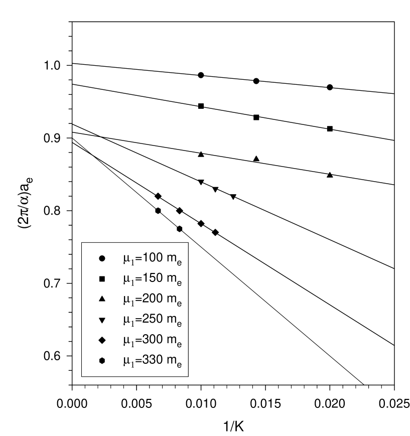
Figure 3: Dependence on longitudinal resolution $K$ of the anomalous moment $a_{e}$ of the electron in units of the Schwinger term ($\alpha/2\pi$) for the two-photon truncation. The PV masses are $m_{1}=2\cdot 10^{4}m_{e}$, $\mu_{1}=100m_{e}$ to $330m_{e}$, and $\mu_{2}=\sqrt{2}\mu_{1}$. The transverse resolution is $N_{\perp}=20$. The lines are linear fits. The errors in the individual points are estimated to be 5%.

The results of the extrapolations are plotted in Fig. 4. Each value is close to the Schwinger result and independent of $\mu_{1}$, to within numerical error. However, there is clearly a systematic tendency to be below the Schwinger result by approximately 10% as the PV photon mass $\mu_{1}$ is increased. We expect that this discrepancy is caused by the absence of two potentially important contributions, the electron-positron loop and the three-photon self-energy. The loop contributes in perturbation theory at the same order in $\alpha$ as the one-electron/two-photon Fock states considered here and corresponds to the addition of two-electron/one-positron Fock states to our truncation. The self-energy contribution is higher order in $\alpha$ but earlier calculations SecDep have shown that the two-photon self-energy is an important correction to the one-photon truncation. This can be seen in Fig. 4, where we reproduce these results for comparison.

Figure 4 also includes results obtained for the two-photon truncation when only the one-loop chiral constraint is satisfied. Without the full nonperturbative constraint, the results are very sensitive to the PV photon mass $\mu_{1}$. This behavior repeats the pattern observed in ChiralLimit for a one-photon truncation without the corresponding one-loop constraint. The resulting $\mu_{1}$ dependence is illustrated in Fig. 2 of ChiralLimit . Thus, a successful calculation requires that the symmetry of the chiral limit be maintained.

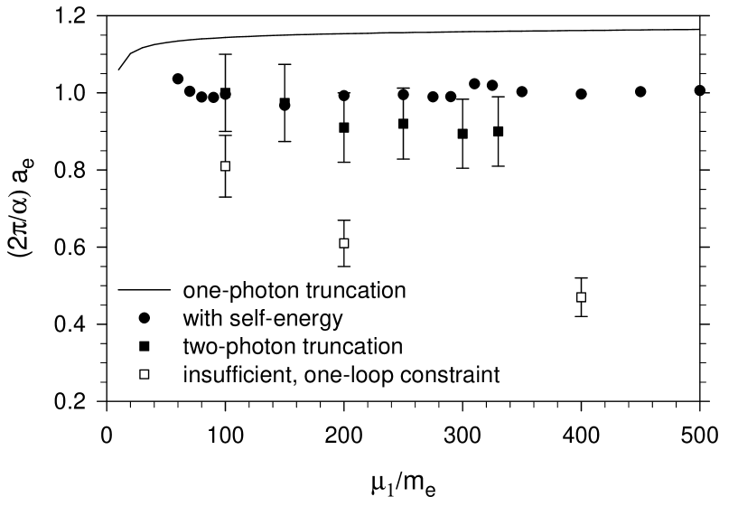
Figure 4: The anomalous moment of the electron in units of the Schwinger term ($\alpha/2\pi$) plotted versus the PV photon mass, $\mu_{1}$, with the second PV photon mass, $\mu_{2}$, set to $\sqrt{2}\mu_{1}$ and the PV electron mass $m_{1}$ equal to $2\cdot 10^{4}\,m_{e}$. The solid squares are the result of the full two-photon truncation with the correct, nonperturbative chiral constraint. The open squares come from use of a perturbative, one-loop constraint. Results for the one-photon truncation ChiralLimit (solid line) and the one-photon truncation with the two-photon self-energy contribution SecDep (filled circles) are included for comparison. The resolutions used for the two-photon results are $K=50$ to 150, combined with extrapolation to $K=\infty$, and $N_{\perp}=20$.

V Summary

The results of the calculation are shown in Fig. 4 and compared with three other calculations: the one-photon truncation ChiralLimit , the one-photon case with the two-photon self-energy contribution SecDep , and the two-photon truncation with only the one-loop chiral constraint. The two-photon results with the correct chiral constraint are consistent with the Schwinger result, and therefore with experiment, to within the estimated numerical error of 10%. The systematic deviation below the Schwinger result is expected to be due to the absence of the two-electron/one-positron Fock sector and the three-photon self-energy contributions. As is well known from perturbation theory, cancellations exist between different types of contributions, such as between photon loops and electron-positron loops, and, therefore, it is not surprising for the present two-photon calculation, which does not also include electron-positron loops, to have a somewhat worse result than the one-photon calculation with just the two-photon self-energy contribution.

Inclusion of an electron-positron pair in the basis is also important for the understanding of current covariance and of nonperturbative renormalization of the charge and photon mass. Future work along these lines will be to include these additional contributions. Of course, the calculation of the anomalous moment is not the important objective; instead, we are interested in testing on QED a nonperturbative method that could be applicable to QCD, to see how the various truncations affect the result and to be able to compare with perturbation theory, as a check.

Further tests of the method within QED could include application to the calculation of a true bound state, positronium Positronium . Just as for the anomalous moment calculation, the positronium results will not be competitive with high-order perturbation theory. The numerical errors are large compared to the tiny perturbative corrections in such a weakly coupled theory. This in turn suggests another interesting test that could be done, a calculation of the anomalous moment when $\alpha$ is much larger that its natural value, yet small enough for perturbation theory to still provide a check.

In a strongly coupled theory, such as QCD, the method may be more quantitative. For QCD, the PV-regulated formulation by Paston et al. Paston could be a starting point. The analog of the dressed-electron problem does not exist, of course, and the minimum truncation that would include non-Abelian effects would be to include at least two gluons. The smallest calculation would then be in the glueball sector. In the meson sector, the minimum truncation would be a quark-antiquark pair plus two gluons, which as a four-body problem would require discretization techniques beyond what are discussed here, since the coupled integral equations for the wave functions cannot be analytically reduced to a single Fock sector. Instead, one would discretize the coupled integral equations directly, in analogy with the original method of DLCQ DLCQreview , and diagonalize a very large but very sparse matrix. As an intermediate step, one can select a less ambitious yet very interesting challenge of modeling the meson sector with effective interactions, particularly with an interaction to break chiral symmetry DalleyMcCartor .

Appendix A Discretizations and quadratures

The integral equations involve integration over the longitudinal momentum fraction and the square of the transverse momentum. The normalization, anomalous moment, and self-energy contributions also require integrals of this form. In each case there can be a line of poles $q_{\rm pole}^{2}$ in the integrand, from the denominators of wave functions in (36), for a range of values of the longitudinal momentum fraction $y$. The location of the line is determined by the energy denominator that appears in each integrand. For simple poles, the transverse momentum integral is defined as the principal value. For those values of longitudinal momentum $y$ for which the pole exists, the $q_{\perp}^{2}$ integration is subdivided into two parts, one from zero to $2q_{\rm pole}^{2}$ and the other from there to infinity. If the pole does not exist, transverse integration is not subdivided. When self-energy effects are included, the location of the pole, if it still exists, must be found by solving a nonlinear equation numerically. We do this with the Müller algorithm BurdenFaires .

For the interval that contains a simple pole, the integral is approximated by an open Newton–Cotes formula that uses a few equally-spaced points placed symmetrically about the pole at $q_{i}^{2}=(2i-1)q_{\rm pole}^{2}/N$ with $i=1,\ldots,N$ and $N$ even. This particular Newton–Cotes formula uses a rectangular approximation to the integrand, with the height equal to the integrand value at the midpoint of an interval of width $2q_{\rm pole}^{2}/N$. An integral is then approximated by

$$\int_{0}^{2q_{\rm pole}^{2}}dq_{\perp}^{2}f(q_{\perp}^{2})\simeq\frac{2q_{\rm pole}^{2}}{N}\sum_{i=1}^{N}f(q_{i}^{2}).$$ (57)

The equally spaced points provide an approximation to the principal value.

This form avoids use of $q_{\perp}^{2}=0$ as a quadrature point. Such a choice is important for evaluating terms with two-photon kernels, where there is another pole associated with the three-particle energy denominator. By keeping $q_{\perp}^{2}$ nonzero, this pole can be handled analytically as a principal value in the angular integration, as discussed in Appendix B.

For the infinite intervals, $q_{\perp}^{2}$ is mapped to a new variable $v$ by the transformation YukawaTwoBoson

$$q_{\perp}^{2}=a^{2}\frac{1-\left(b^{2}/a^{2}\right)^{v}}{\left(b^{2}/a^{2}\right)^{v-1}-1},$$ (58)

with $v$ in the range 0 to 1. (If the pole exists, this transformation is shifted by $2q_{\rm pole}^{2}$.) The PV contributions make the integrals finite; therefore, no transverse cutoff is needed. Only the positive Gauss–Legendre quadrature points of an even order $2N_{\perp}$ are used for $v$ between -1 and 1, so that $v=0$, and therefore $q^{\prime}_{\perp}=0$ (or $2q_{\rm pole}^{2}$), is never a quadrature point. The points in the negative half of the range, which would be used for representing $q_{\perp}^{2}\in[-\infty,0]$, are discarded. One could map $q_{\perp}^{2}\in[0,\infty]$ to $[-1,1]$ and not discard any part of the Gauss–Legendre range; however, the quadrature would then place points focused on some finite $q_{\perp}^{2}$ value, rather than on the natural integrand peak at $q_{\perp}^{2}=0$. The total number of quadrature points in the transverse direction is $N_{\perp}+N$, with $N=0$ when there is no pole and $N_{\perp}$ typically of order 20.

This transformation was used in YukawaTwoBoson and was selected to obtain an exact result for the integral $\int[1/(a^{2}+q^{2})-1/(b^{2}+q^{2})]dq^{2}$. In the present work, the scales $a^{2}$ and $b^{2}$ are chosen to be the smallest and largest scales in the problem, i.e. $a^{2}=|q_{\rm pole}^{2}|$ and $b^{2}=m_{1}^{2}y+\mu_{1}^{2}(1-y)-M^{2}y(1-y)$. Here $q_{\rm pole}^{2}$ is the location of the root of the nonlinear equation for the pole. If $q_{\rm pole}^{2}$ is negative, a pole does not exist; however, $|q_{\rm pole}^{2}|$ is still a natural scale for the integrand.

For the normalization and anomalous moment integrals, the transverse quadrature scheme is based on a different transformation

$$q_{\perp}^{2}=a^{2}\frac{v}{1-v},$$ (59)

where, again, if the pole exists, the transformation is shifted by $2q_{\rm pole}^{2}$. Cubic-spline interpolation BurdenFaires is then used to compute the values of the wave functions at the new quadrature points. This transformation is selected to yield an exact result for the integral of $1/(a^{2}+q^{2})^{2}$, which is the form of the dominant contribution to the normalization and anomalous moment.

The longitudinal integration is subdivided into three parts when the line of poles is present. Two parts are symmetrically placed about the logarithmic singularity at $y_{\rm pole}$ that arises where the line of poles reaches $q_{\perp}^{2}=0$. When self-energy effects are not included in the energy denominator, this occurs at $y_{\rm pole}=1-m_{0}^{2}/M^{2}$; when self-energy effects are present, the location must be found by solving a nonlinear equation. The third part of the integration covers the remainder of the unit interval. Specifically, these intervals are $[0,y_{\rm pole}]$, $[y_{\rm pole},2y_{\rm pole}]$, and $[2y_{\rm pole},1]$. This structure is designed to maintain a left-right symmetry around the logarithmic singularity, because in the normalization and anomalous moment integrals (which use the same longitudinal quadrature points) the singularity becomes a simple pole defined by a principal-value prescription. The left-right symmetry then assures the necessary cancellations from opposite sides of the pole. When no pole is present, the longitudinal integration is not subdivided.

The intervals are each mapped linearly to $\tilde{y}\in[0,1]$ and then altered by the transformations YukawaTwoBoson

$$\tilde{y}(t)=t^{3}(1+dt)/[1+d-(3+4d)t+(3+6d)t^{2}-4dt^{3}+2dt^{4}]$$ (60)

and

$$t(u)=(u+1)/2.$$ (61)

The new variable $u$ ranges between -1 and 1, and standard Gauss–Legendre quadrature is applied. The transformation from $\tilde{y}$ to $t$ is constructed to concentrate many points near the end-points of each interval, where integrands are rapidly varying. The parameter $d$ is chosen such that $\tilde{y}\simeq 0.01t^{3}$ for small $t$. The transformation was found empirically YukawaTwoBoson , beginning with a transformation constructed to compute the integral $\int_{0}^{1}[\ln(y+\epsilon_{0})-\ln(y+\epsilon_{1})]dy$ exactly, with $\epsilon_{0}$ and $\epsilon_{1}$ small. The symmetry with respect to the replacements $t\rightarrow(1-t)$ and $\tilde{y}\rightarrow(1-\tilde{y})$ is not necessary but is the simplest choice for restricting the coefficients in the denominator of (60).

The need for a concentration of longitudinal quadrature points near 0 and 1 is particularly true for the integral $\bar{J}$, defined in (78). Although this integral can be done analytically for the case of the one-photon truncation discussed in ChiralLimit , the integral is only implicit in the integral equations for the two-body wave functions discussed in Sec. III and must therefore be well represented by any discretization of the integral equations. After the transverse integration is performed, the integrand is sharply peaked near $y=0$ and $y=1$, at distances of order $m_{0}/m_{1}\sim 10^{-10}$ from these end-points, and needs to be sampled on both sides of the peaks.

The number of points in each of the three intervals is denoted by $K$, which becomes the measure of the resolution analogous to the harmonic resolution of DLCQ PauliBrodsky . Thus the total number of quadrature points in the longitudinal direction is $3K$, with $K$ typically of order 50 or higher.

For those longitudinal integrals with an upper limit less than 1, the integrand is transformed as above and given a value of zero for the points beyond the original integration range.

For the normalization and anomalous moment integrals, the pole in the transverse integral (when it exists) is a double pole, defined by the limit OnePhotonQED

$$\int dy\;dq_{\perp}^{2}\;\frac{f(y,q_{\perp}^{2})}{[m^{2}y+\mu_{0}^{2}(1-y)-M^{2}y(1-y)+q_{\perp}^{2}]^{2}}$$

$$\equiv\lim_{\epsilon\rightarrow 0}{\frac{1}{2}\epsilon}\int dy\int dq_{\perp}^{2}f(y,k_{\perp}^{2})\Bigg{[}\frac{1}{[m^{2}y+\mu_{0}^{2}(1-y)-M^{2}y(1-y)+q_{\perp}^{2}-\epsilon]}$$

$$-\frac{1}{[m^{2}y+\mu_{0}^{2}(1-y)-M^{2}y(1-y)+q_{\perp}^{2}+\epsilon]}\Bigg{]}.$$ (62)

The simple poles that remain are prescribed as principal values. Of course, the limit must be taken after the integral is performed.

This limiting process is taken into account numerically by using a quadrature formula that is specific to this double-pole form. On the interval $[0,2q_{\rm pole}^{2}]$, the quadrature points are chosen to be the same as those used for the integral equations, which are $q_{i}^{2}=(2i-1)q_{\rm pole}^{2}/N$ with $i=1,\ldots,N$, as given above. The interval is divided into $N/2$ subintervals $[\frac{4m}{N}q_{\rm pole}^{2},\frac{4(m+1)}{N}q_{\rm pole}^{2}]$, with $m=0,1,\ldots,(N-2)/2$, each containing two of the quadrature points. The quadrature formula for such a subinterval is taken to be

$$\int_{\frac{4m}{N}q_{\rm pole}^{2}}^{\frac{4(m+1)}{N}q_{\rm pole}^{2}}dq_{\perp}^{2}\frac{f(q_{\perp}^{2})}{(q_{\perp}^{2}-q_{\rm pole}^{2})^{2}}\simeq w_{2m+1}f(\frac{(4m+1)}{N}q_{\rm pole}^{2})+w_{2m+2}f(\frac{(4m+3)}{N}q_{\rm pole}^{2}),$$ (63)

where the integral on the left is defined by the limit formula in (A) when the pole is in the subinterval. The weights $w_{i}$ are chosen to make the formula exact for $f=1$ and $f=q_{\perp}^{2}$ on each individual $q_{\perp}^{2}$ subinterval. For these numerator functions, the limit in (A) can be taken explicitly. The weights are then found to be $w_{N/2}=w_{N/2+1}=-N/2q_{\rm pole}^{2}$, for the quadrature points on either side of the pole. For all other points, the weights are given by

$$w_{2m+1} = -\frac{N}{2q_{\rm pole}^{2}}\left[\ln\left|\frac{4m+4-N}{4m-N}\right|+\frac{4(N-4m-3)}{(4m-N)(4m+4-N)}\right],$$ (64)

$$w_{2m+2} = \frac{N}{2q_{\rm pole}^{2}}\left[\ln\left|\frac{4m+4-N}{4m-N}\right|+\frac{4(N-4m-1)}{(4m-N)(4m+4-N)}\right].$$

The integral from 0 to $2q_{\rm pole}^{2}$ is obtained by summing over the individual subintervals.

For the self-energy contribution (25), which is expressed in terms of the integrals $\bar{I}_{0}$, $\bar{I}_{1}$, and $\bar{J}=M^{2}\bar{I}_{0}$ given in (77) and (78), the transverse integral is done analytically. Only the longitudinal integral is done numerically, by the scheme discussed above with resolution $K=30$.

Appendix B Angular integrals

Calculation of the two-photon kernels requires the integrals

$${\cal I}_{n}=\int_{0}^{2\pi}\frac{d\phi}{2\pi}\frac{e^{-in\phi}}{D+F\cos\phi},$$ (65)

first defined in Eq. (22), with $D$ and $F$ given in (23). Here the original integration variable $\phi^{\prime}$ has been shifted by the independent angle $\phi$, and the prime then dropped for simplicity of notation in this Appendix. The factor $F$ is always positive, but $D$ can be negative. If the bare fermion mass $m_{0}$ is less than the physical mass $m_{e}$, we can have $|D|<F$; in this case, ${\cal I}_{n}$ is defined by a principal value, as in the one-photon sector. If either photon has zero transverse momentum, $F$ will be zero, and any pole due to a zero in $D$ will not involve the angular integration. The numerical quadrature is chosen to never use grid points where a photon transverse momentum is zero, so that the principal-value prescription can always be invoked for the angular integral, where it is easily handled analytically.

The imaginary part of ${\cal I}_{n}$ is zero. This follows from the even parity of the denominator and the odd parity of $\sin n\phi$. As a consequence, ${\cal I}_{-n}={\cal I}_{n}$, and we evaluate (65) for only nonnegative $n$.

The real part is nonzero and most easily calculated from combinations of the related integrals

$$\bar{\cal I}_{n}=\int_{0}^{2\pi}\frac{d\phi}{2\pi}\frac{\cos^{n}\phi}{D+F\cos\phi}.$$ (66)

Of course, for $n=0$ and 1, the two integrals are identical. For $n=2$ and 3 we have $\cos 2\phi=2\cos^{2}\phi-1$ and $\cos 3\phi=4\cos^{3}\phi-3\cos\phi$. Therefore, the integral combinations are

$${\cal I}_{0}=\bar{\cal I}_{0},\;\;{\cal I}_{1}=\bar{\cal I}_{1},\;\;{\cal I}_{2}=2\bar{\cal I}_{2}-\bar{\cal I}_{0},\;\;{\cal I}_{3}=4\bar{\cal I}_{3}-3\bar{\cal I}_{1}.$$ (67)

Larger values of $n$ do not appear in the two-photon kernels.

The integrals $\bar{\cal I}_{n}$ are connected by a simple recursion for $n>0$:

$$\bar{\cal I}_{n}=\int_{0}^{2\pi}\frac{d\phi}{2\pi}\frac{\cos^{n-1}\phi}{F}\frac{(D+F\cos\phi-D)}{D+F\cos\phi}=\frac{1}{F}\int_{0}^{2\pi}\frac{d\phi}{2\pi}\cos^{n-1}\phi-\frac{D}{F}\bar{\cal I}_{n-1}.$$ (68)

The first term is zero when $n$ is even. For $n=1$, it is $1/F$, and for $n=3$, this term is $1/2F$. The only other integral that must be evaluated directly is $\bar{\cal I}_{0}={\cal I}_{0}$.

The determination of ${\cal I}_{0}$, with or without the presence of poles, is conveniently done by contour integration around the unit circle in terms of a complex variable $z=e^{i\phi}$. We then have

$${\cal I}_{0}=\frac{1}{i\pi F}\oint\frac{dz}{z^{2}+2\frac{D}{F}z+1}=\frac{1}{i\pi F}\oint\frac{dz}{(z-z_{+})(z-z_{-})}.$$ (69)

There are simple poles at

$$z_{\pm}=-\frac{D}{F}\pm\sqrt{\frac{D^{2}}{F^{2}}-1}=-\frac{D}{F}\pm i\sqrt{1-\frac{D^{2}}{F^{2}}}=-e^{\mp i\cos^{-1}(D/F)}$$ (70)

When $D$ is greater than $F$, one pole, $z_{+}$, is inside the contour and the other outside, as illustrated in Fig. 5.

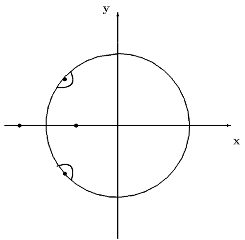
Figure 5: Integration contour for evaluation of ${\cal I}_{0}$. The locations of the poles at $z_{\pm}$ depend upon the magnitude and sign of $D/F$. The semicircles are used when $|D|/F<1$ and the poles are on the contour.

Evaluation of $2\pi i$ times the residue yields

$${\cal I}_{0}=\frac{1}{\sqrt{D^{2}-F^{2}}}\;\;\mbox{for}\;\;D>F.$$ (71)

Similarly, when $D$ is less than $-F$, the pole at $z_{-}$ is inside the contour, and we have

$${\cal I}_{0}=-\frac{1}{\sqrt{D^{2}-F^{2}}}\;\;\mbox{for}\;\;D<-F.$$ (72)

When $|D|$ is less than $F$, the poles move to the contour, and the integral is defined by the principal value. This is evaluated by distorting the contour to include semicircles of radius $\epsilon$ around each pole, as shown in Fig. 5, and subtracting the contributions from the semicircles after taking the $\epsilon\rightarrow 0$ limit. The choice of inward semicircles makes the integral around the closed contour simply zero. For the semicircle around $z_{\pm}$, we have $z=z_{\pm}+\epsilon e^{i\theta}$ and a contribution, as $\epsilon$ goes to zero, of

$$\frac{2}{iF}\int\frac{\epsilon ie^{i\theta}d\theta}{\epsilon e^{i\theta}(\epsilon e^{i\theta}\mp 2i\sqrt{1-D^{2}/F^{2}})}\longrightarrow\frac{\pm\int d\theta}{F\sqrt{1-D^{2}/F^{2}}}.$$ (73)

Thus the contributions from the two semicircles are of opposite sign and cancel, so that the net result is also zero. Therefore, we have

$${\cal I}_{0}=\left\{\begin{array}[]{ll}\frac{1}{\sqrt{D^{2}-F^{2}}},&D>F\\ 0,&|D|<F\\ -\frac{1}{\sqrt{D^{2}-F^{2}}},&D<-F.\end{array}\right.$$ (74)

The case where $D$ equals $F$ represents an integrable singularity for the transverse momentum integrations and can be ignored. When $F$ is zero, we have simply

$${\cal I}_{n}=\int_{0}^{2\pi}\frac{d\phi}{2\pi D}e^{-in\phi}=\frac{1}{D}\delta_{n0}.$$ (75)

When $F/D$ is small, the expressions for the integrals ${\cal I}_{n}$ are best evaluated from expansions in powers of $F/D$, to avoid round-off errors due to cancellations between large contributions. The expansions used are

$${\cal I}_{0} \simeq \frac{1}{128D}\left[128+64\left(\frac{F}{D}\right)^{2}+48\left(\frac{F}{D}\right)^{4}+40\left(\frac{F}{D}\right)^{6}+35\left(\frac{F}{D}\right)^{8}\right],$$ (76)

$${\cal I}_{1} \simeq -\frac{1}{128D}\left(\frac{F}{D}\right)\left[64+48\left(\frac{F}{D}\right)^{2}+40\left(\frac{F}{D}\right)^{4}+35\left(\frac{F}{D}\right)^{6}\right],$$

$${\cal I}_{2} \simeq \frac{1}{128D}\left(\frac{F}{D}\right)^{2}\left[32+32\left(\frac{F}{D}\right)^{2}+30\left(\frac{F}{D}\right)^{4}\right],$$

$${\cal I}_{3} \simeq -\frac{1}{128D}\left(\frac{F}{D}\right)^{3}\left[16+20\left(\frac{F}{D}\right)^{2}\right].$$

Appendix C Numerical convergence

The primary constraint on numerical accuracy is the error in the estimation of the integrals in the integral equations for the wave functions and in the expressions for the normalization and the anomalous moment. This accuracy is determined by the choice of quadrature scheme, discussed in Appendix A, and the resolution, controlled by the longitudinal parameter $K$ and transverse parameter $N_{\perp}$. The other numerical parts of the calculation are iterated to what is effectively exact convergence, with remaining uncertainties much smaller than the errors in the numerical quadratures.

Table 1: Dependence on longitudinal resolution $K$ of the integrals $\bar{I}_{0}$, $\bar{I}_{1}$, and $\bar{J}$, defined in (77) and (78) of the text and computed according to the quadrature scheme described in Appendix A. The bare-electron mass is $m_{0}=0.98m_{e}$. The PV masses are $m_{1}=2\cdot 10^{4}m_{e}$, $\mu_{1}=200m_{e}$, and $\mu_{2}=\sqrt{2}\mu_{1}$. The transverse resolution is $N_{\perp}=40$.

$K$	$\bar{I}_{0}(m_{e}^{2})$	$\bar{I}_{1}(m_{e}^{2})/m_{e}$	$\bar{J}(m_{e}^{2})/m_{e}^{2}$
5	-7.113	-13.530	-11606.
10	-6.2586	-10.6182	932.3
15	-6.2641	-10.7354	-26.487
20	-6.2645	-10.7327	-6.7126
25	-6.2645	-10.7328	-6.3982
30	-6.2645	-10.7328	-6.4401
exact	-6.2645	-10.7328	-6.2645

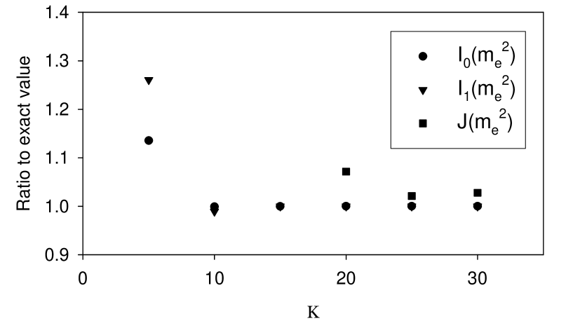
Figure 6: Dependence on longitudinal resolution $K$ of the integrals $I_{0}$, $I_{1}$, and $J$, defined in (77) and (78) of the text and computed according to the quadrature scheme described in Appendix A. The values plotted are ratios to the exact values, listed in Table 1. The bare-electron mass is $m_{0}=0.98m_{e}$. The PV masses are $m_{1}=2\cdot 10^{4}m_{e}$, $\mu_{1}=200m_{e}$, and $\mu_{2}=\sqrt{2}\mu_{1}$. The transverse resolution is $N_{\perp}=40$.

Table 2: Same as Table 1, but for the dependence on transverse resolution $N_{\perp}$. The longitudinal resolution is $K=30$.

$N_{\perp}$	$\bar{I}_{0}(m_{e}^{2})$	$\bar{I}_{1}(m_{e}^{2})/m_{e}$	$\bar{J}(m_{e}^{2})/m_{e}^{2}$
10	-6.2646	-10.7324	-2.9845
15	-6.2645	-10.7327	-7.5428
20	-6.2645	-10.7327	-6.9137
25	-6.2645	-10.7328	-6.6961
30	-6.2645	-10.7328	-6.5712
35	-6.2645	-10.7328	-6.4922
40	-6.2645	-10.7328	-6.4401
exact	-6.2645	-10.7328	-6.2645

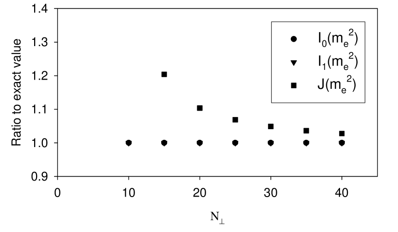
Figure 7: Same as Fig. 6, but for the dependence on transverse resolution $N_{\perp}$. The longitudinal resolution is $K=30$. For these resolutions, the values for $\bar{I}_{0}$ and $\bar{I}_{1}$ are nearly exact, and the plotted points for the ratios to the exact values are at the same places; only $J$ shows variation.

For the one-photon truncation, discussed in OnePhotonQED and ChiralLimit , all the integrals can be done analytically. This makes the one-photon problem a convenient first test for numerical convergence. The key integrals are $\bar{I}_{0}$, $\bar{I}_{1}$, and $\bar{J}$, defined as

$$\bar{I}_{n}(M^{2}) = \int\frac{dydk_{\perp}^{2}}{16\pi^{2}}\sum_{jl}\frac{(-1)^{j+l}\xi_{l}}{M^{2}-\frac{m_{j}^{2}+k_{\perp}^{2}}{1-y}-\frac{\mu_{l}^{2}+k_{\perp}^{2}}{y}}\frac{m_{j}^{n}}{y(1-y)^{n}}\,,$$ (77)

$$\bar{J}(M^{2}) = \int\frac{dydk_{\perp}^{2}}{16\pi^{2}}\sum_{jl}\frac{(-1)^{j+l}\xi_{l}}{M^{2}-\frac{m_{j}^{2}+k_{\perp}^{2}}{1-y}-\frac{\mu_{l}^{2}+k_{\perp}^{2}}{y}}\frac{m_{j}^{2}+k_{\perp}^{2}}{y(1-y)^{2}}.$$ (78)

Tables 1 and 2 and Figs. 6 and 7 summarize results for numerical calculation of these integrals. They show that $\bar{I}_{0}$ and $\bar{I}_{1}$ are well approximated for a wide range of resolutions, but $\bar{J}$ is particularly sensitive to the longitudinal resolution $K$ and requires that both $K$ and $N_{\perp}$ be on the order of 20 or larger. At these resolutions, $\bar{J}$ is approximated with an accuracy of about 4%, and this then becomes a minimal estimate of the accuracy of any of the results.

Table 3: Dependence on longitudinal resolution $K$ of the bare mass $m_{0}$ and anomalous moment $a_{e}$ of the electron in units of the physical mass $m_{e}$ and the Schwinger term ($\alpha/2\pi$), respectively, for both the one-photon truncation, when solved numerically, and the case with the self-energy included. The value of the bare mass is obtained as the value that yields a physical value of the coupling constant $\alpha$; for $K=15$, two solutions are found. The PV masses are $m_{1}=2\cdot 10^{4}m_{e}$, $\mu_{1}=200m_{e}$, and $\mu_{2}=\sqrt{2}\mu_{1}$. The transverse resolution is $N_{\perp}=40$.

	one-photon		with self-energy
$K$	$m_{0}/m_{e}$	$2\pi a_{e}/\alpha$	$m_{0}/m_{e}$	$2\pi a_{e}/\alpha$
5	4.4849	0.09921	4.4845	0.09444
10	1.7445	0.22992	1.7106	0.22620
15	1.07487	0.64482	1.07481	0.59092
15	0.98906	1.12763	0.97537	1.07444
20	0.98223	1.15430	0.99028	0.90337
25	0.98240	1.15382	0.98295	0.99242
30	0.98241	1.15567	0.98245	1.00612

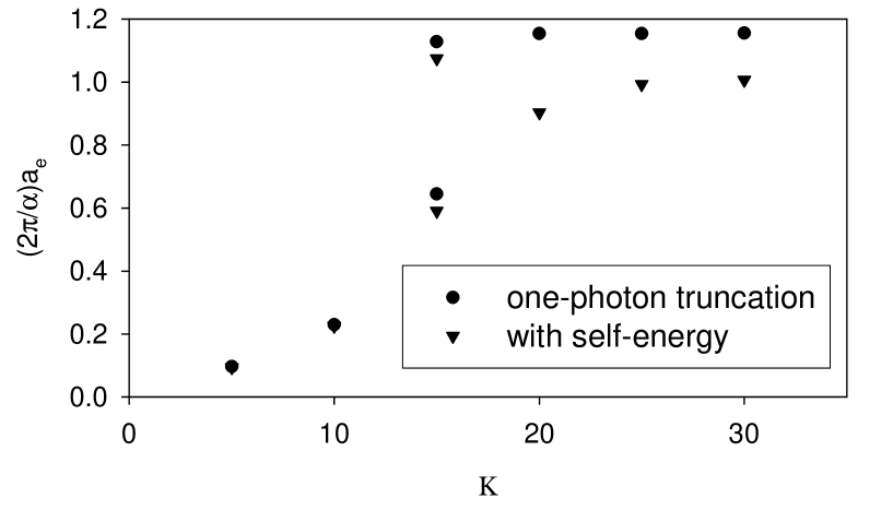
Figure 8: Dependence on longitudinal resolution $K$ of the anomalous moment $a_{e}$ of the electron in units of the Schwinger term ($\alpha/2\pi$) for both the one-photon truncation, when solved numerically, and the case with the self-energy included. The PV masses are $m_{1}=2\cdot 10^{4}m_{e}$, $\mu_{1}=200m_{e}$, and $\mu_{2}=\sqrt{2}\mu_{1}$. The transverse resolution is $N_{\perp}=40$.

Table 4: Same as Table 3, but for the dependence on transverse resolution $N_{\perp}$. The longitudinal resolution is $K=30$.

	one-photon		with self-energy
$N_{\perp}$	$m_{0}/m_{e}$	$2\pi a_{e}/\alpha$	$m_{0}/m_{e}$	$2\pi a_{e}/\alpha$
10	0.98023	1.16121	0.97918	—
15	0.98297	1.15317	0.98307	0.99071
20	0.98268	1.15380	0.98275	0.99776
25	0.98256	1.15484	0.98261	1.00130
30	0.98248	1.15399	0.98253	1.00348
35	0.98244	1.15404	0.98248	1.00501
40	0.98241	1.15567	0.98245	1.00612

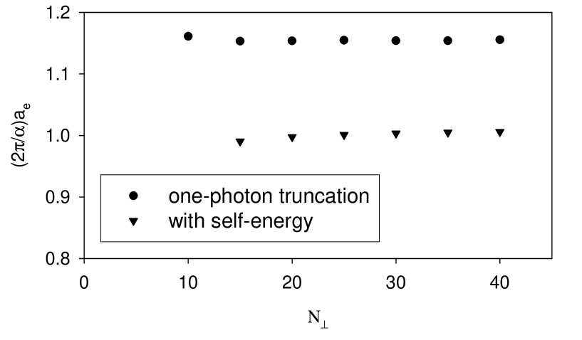
Figure 9: Same as Fig. 8, but for the dependence on transverse resolution $N_{\perp}$. The longitudinal resolution is $K=30$.

As expected, the results for the one-photon truncation, if computed numerically, converge to better than 1% at the same resolution, of $K=20$ and $N_{\perp}=20$, as can be seen in Tables 3 and 4 and Figs. 8 and 9. However, the results with the self-energy contribution, shown in the same tables and figures, require $K\simeq 25$ before nearing convergence. Although the exact answer is not known in this case, $K=20$ is clearly insufficient, but $K\gg 25$ yields a reasonable result with an error on the order of 1%.

The two-photon truncation incorporates numerical approximations to the integrals $\bar{I}_{0}$, $\bar{I}_{1}$, and $\bar{J}$ through the action of the zero-photon kernel $J^{(0)}$, in Eq. (III.1), and approximations to the self-energy contribution, also in Eq. (III.1). Thus, the minimum resolution for the two-photon calculation would appear to be approximately $K=25$ and $N_{\perp}=20$; however, we find that $K$ must be at least 50. We extrapolate from the one-photon and self-energy calculations to estimate an error of 5-10% for the two-photon truncation.

References

- (1) T. Kinoshita and M. Nio, Phys. Rev. D 73, 013003 (2006).
- (2) S.J. Brodsky, J.R. Hiller, and G. McCartor, Phys. Rev. D 58, 025005 (1998).
- (3) S.J. Brodsky, J.R. Hiller, and G. McCartor, Phys. Rev. D 60, 054506 (1999).
- (4) S.J. Brodsky, J.R. Hiller, and G. McCartor, Phys. Rev. D 64, 114023 (2001).
- (5) S.J. Brodsky, J.R. Hiller, and G. McCartor, Ann. Phys. 296, 406 (2002).
- (6) S.J. Brodsky, J.R. Hiller, and G. McCartor, Ann. Phys. 305, 266 (2003).
- (7) S.J. Brodsky, V.A. Franke, J.R. Hiller, G. McCartor, S.A. Paston, and E.V. Prokhvatilov, Nucl. Phys. B 703, 333 (2004).
- (8) S.J. Brodsky, J.R. Hiller, and G. McCartor, Ann. Phys. 321, 1240 (2006).
- (9) S.S. Chabysheva and J.R. Hiller, Phys. Rev. D 79, 114017 (2009).
- (10) S.S. Chabysheva, A nonperturbative calculation of the electron’s anomalous magnetic moment, Ph.D. thesis, Southern Methodist University [ProQuest Dissertations & Theses 3369009, 2009].
- (11) S.S. Chabysheva and J.R. Hiller, Ann. Phys. 325, 2435 (2010).
- (12) H.-C. Pauli and S.J. Brodsky, Phys. Rev. D 32, 1993 (1985); 32, 2001 (1985).
- (13) J.P. Vary et al., Phys. Rev. C 81, 035205 (2010).
- (14) C. Lanczos, J. Res. Nat. Bur. Stand. 45, 255 (1950); J.H. Wilkinson, The Algebraic Eigenvalue Problem (Clarendon, Oxford, 1965); B.N. Parlett, The Symmetric Eigenvalue Problem (Prentice-Hall, Englewood Cliffs, NJ, 1980); D.S. Scott, in Sparse Matrices and their Uses, edited by I.S. Duff (Academic Press, London, 1981), p. 139; G.H. Golub and C.F. van Loan, Matrix Computations (Johns Hopkins University Press, Baltimore, 1983); J. Cullum and R.A. Willoughby, in Large-Scale Eigenvalue Problems, eds. J. Cullum and R.A. Willoughby, Math. Stud. 127 (Elsevier, Amsterdam, 1986), p. 193; Y. Saad, Comput. Phys. Commun. 53, 71 (1989); S.K. Kin and A.T. Chronopoulos, J. Comp. and Appl. Math. 42, 357 (1992).
- (15) J. Cullum and R.A. Willoughby, J. Comput. Phys. 44, 329 (1981); Lanczos Algorithms for Large Symmetric Eigenvalue Computations (Birkhauser, Boston, 1985), Vol. I and II.
- (16) W. Pauli and F. Villars, Rev. Mod. Phys. 21, 434 (1949).
- (17) B. Grinstein, D. O’Connell, and M.B. Wise, Phys. Rev. D 77, 025012 (2008); C.D. Carone and R.F. Lebed, JHEP 0901:043 (2009).
- (18) P.A.M. Dirac, Rev. Mod. Phys. 21, 392 (1949).
- (19) For reviews and additional references, see M. Burkardt, Adv. Nucl. Phys. 23, 1 (2002); S.J. Brodsky, H.-C. Pauli, and S.S. Pinsky, Phys. Rep. 301, 299 (1998).
- (20) K. Hornbostel, S. J. Brodsky and H. C. Pauli, Phys. Rev. D 41, 3814 (1990).
- (21) Y. Matsumura, N. Sakai, and T. Sakai, Phys. Rev. D 52, 2446 (1995); O. Lunin and S. Pinsky, AIP Conf. Proc. 494, 140 (1999); J. R. Hiller, S. S. Pinsky, N. Salwen and U. Trittmann, Phys. Lett. B 624, 105 (2005) and references therein.
- (22) L.C.L. Hollenberg, K. Higashijima, R.C. Warner, and B.H.J. McKellar, Prog. Th. Phys. 87, 441 (1992).
- (23) I. Tamm, J. Phys. (Moscow) 9, 449 (1945); S.M. Dancoff, Phys. Rev. 78, 382 (1950).
- (24) R.J. Perry, A. Harindranath, and K.G. Wilson, Phys. Rev. Lett. 65, 2959 (1990); R.J. Perry and A. Harindranath, Phys. Rev. D 43, 4051 (1991).
- (25) K.G. Wilson, T.S. Walhout, A. Harindranath, W.-M. Zhang, R.J. Perry, and St.D. Głazek, Phys. Rev. D 49, 6720 (1994);
- (26) A. Harindranath and R.J. Perry, Phys. Rev. D 43, 492 (1991); 43, 3580(E) (1991); D. Mustaki, S. Pinsky, J. Shigemitsu, and K.G. Wilson, ibid. 43, 3411 (1991); A. Langnau, Ph.D. thesis, SLAC Report 385, 1992; A. Langnau and S.J. Brodsky, J. Comput. Phys. 109, 84 (1993); R.J. Perry, Phys. Lett. B300, 8 (1993); W.-M. Zhang and A. Harindranath, Phys. Rev. D 48, 4868 (1993); 48, 4881 (1993); A. Harindranath and W.-M. Zhang, Phys. Rev. D 48, 4903 (1993); N.E. Ligterink and B.L.G. Bakker, Phys. Rev. D 52, 5917 (1995); 52, 5954 (1995); N.C.J. Schoonderwoerd and B.L.G. Bakker, Phys. Rev. D 57, 4965 (1998); 58, 025013 (1998).
- (27) For a perturbative analysis using light-cone quantization, see A. Langnau, Ph.D. thesis, SLAC Report 385, 1992; A. Langnau and M. Burkardt, Phys. Rev. D 47, 3452 (1993).
- (28) A.C. Tang, S.J. Brodsky, and H.-C. Pauli, Phys. Rev. D 44, 1842 (1991).
- (29) J. Schwinger, Phys. Rev. 73, 416 (1948); 76, 790 (1949).
- (30) C.M. Sommerfield, Phys. Rev. 107, 328 (1957); A. Petermann, Helv. Phys. Acta. 30, 407 (1957).
- (31) See, for example, S. Capstick and N. Isgur, Phys. Rev. D 34, 2809 (1986); S. Godfrey and N. Isgur, Phys. Rev. D 32, 189 (1985).
- (32) M.M. Brisudova, R.J. Perry, and K.G. Wilson, Phys. Rev. Lett. 78, 1227 (1997).
- (33) S. J. Brodsky and G. F. de Teramond, Phys. Rev. Lett. 96, 201601 (2006).
- (34) S. D. Głazek and J. Mlynik, Phys. Rev. D 74, 105015 (2006), S. D. Głazek, Phys. Rev. D 69, 065002 (2004), S. D. Głazek and J. Mlynik, Phys. Rev. D 67, 045001 (2003); St.D. Głazek and M. Wieckowski, Phys. Rev. D 66, 016001 (2002).
- (35) J.R. Hiller and S.J. Brodsky, Phys. Rev. D 59, 016006 (1998).
- (36) V. A. Karmanov, J. F. Mathiot, and A. V. Smirnov, Phys. Rev. D 77, 085028 (2008).
- (37) For reviews, see M. Creutz, L. Jacobs and C. Rebbi, Phys. Rep. 95, 201 (1983); J.B. Kogut, Rev. Mod. Phys. 55, 775 (1983); I. Montvay, ibid. 59, 263 (1987); A.S. Kronfeld and P.B. Mackenzie, Ann. Rev. Nucl. Part. Sci. 43, 793 (1993); J.W. Negele, Nucl. Phys. A553, 47c (1993); K.G. Wilson, Nucl. Phys. B (Proc. Suppl.) 140, 3 (2005); J.M. Zanotti, PoS LAT2008, 007 (2008). For recent discussions of meson properties and charm physics, see for example C. McNeile and C. Michael [UKQCD Collaboration], Phys. Rev. D 74, 014508 (2006); I. Allison et al. [HPQCD Collaboration], Phys. Rev. D 78, 054513 (2008).
- (38) M. Burkardt and S. Dalley, Prog. Part. Nucl. Phys. 48, 317 (2002) and references therein; S. Dalley and B. van de Sande, Phys. Rev. D 67, 114507 (2003); D. Chakrabarti, A.K. De, and A. Harindranath, Phys. Rev. D 67, 076004 (2003); M. Harada and S. Pinsky, Phys. Lett. B 567, 277 (2003); S. Dalley and B. van de Sande, Phys. Rev. Lett. 95, 162001 (2005); J. Bratt, S. Dalley, B. van de Sande, and E. M. Watson, Phys. Rev. D 70, 114502 (2004). For work on a complete light-cone lattice, see C. Destri and H.J. de Vega, Nucl. Phys. B290, 363 (1987); D. Mustaki, Phys. Rev. D 38, 1260 (1988).
- (39) C.D. Roberts and A.G. Williams, Prog. Part. Nucl. Phys. 33, 477 (1994); P. Maris and C.D. Roberts, Int. J. Mod. Phys. E12, 297 (2003); P.C. Tandy, Nucl. Phys. B (Proc. Suppl.) 141, 9 (2005).
- (40) S.J. Brodsky, R. Roskies, and R. Suaya, Phys. Rev. D 8, 4574 (1973).
- (41) S.J. Brodsky and S.D. Drell, Phys. Rev. D 22, 2236 (1980).
- (42) R.L. Burden and J.D. Faires, Numerical Analysis, 3rd ed., (Prindle, Weber & Schmidt, Boston, 1985).
- (43) D. Klabucar and H.-C. Pauli, Z. Phys. C 47, 141 (1990); M. Kaluža and H.-C. Pauli, Phys. Rev. D 45, 2968 (1992); M. Krautgärtner, H.C. Pauli, and F. Wölz, ibid. 45, 3755 (1992); U. Trittmann and H.-C. Pauli, hep-th/9704215; hep-th/9705021; U. Trittmann, hep-th/9705072; hep-th/9706055.
- (44) S.A. Paston and V.A. Franke, Theor. Math. Phys. 112, 1117 (1997) [Teor. Mat. Fiz. 112, 399 (1997)]; S.A. Paston, V.A. Franke, and E.V. Prokhvatilov, Theor. Math. Phys. 120, 1164 (1999) [Teor. Mat. Fiz. 120, 417 (1999)].
- (45) S. Dalley and G. McCartor, Ann. Phys. 321, 402 (2006).