High energy emission components in the short GRB 090510

Abstract

We investigate the origin of the prompt and delayed emission observed in the short GRB 090510. We use the broad-band data to test whether the most popular theoretical models for gamma-ray burst emission can accommodate the observations for this burst. We first attempt to explain the soft-to-hard spectral evolution associated with the delayed onset of a GeV tail with the hypothesis that the prompt burst and the high energy tail both originate from a single process, namely synchrotron emission from internal shocks. Considerations on the compactness of the source imply that the high-energy tail should be produced in a late-emitted shell, characterized by a Lorentz factor greater than the one generating the prompt burst. However, in this hypothesis, the predicted evolution of the synchrotron peak frequency does not agree with the observed soft-to-hard evolution. Given the difficulties of a single-mechanism hypothesis, we test two alternative double-component scenarios. In the first, the prompt burst is explained as synchrotron radiation from internal shocks, and the high energy emission (up to about 1 s following the trigger) as internal shock synchrotron-self-Compton. In the second scenario, in view of its long duration ($\sim 100$ s), the high energy tail is decoupled from the prompt burst and has an external shock origin. In this case, we show that a reasonable choice of parameters does indeed exist to accommodate the optical-to-GeV data, provided the Lorentz factor of the shocked shell is sufficiently high. Finally, we attempt to explain the chromatic break observed around $\sim 10^{3}$ s with a structured jet model. We find that this might be a viable explanation, and that it lowers the high value of the burst energy derived assuming isotropy, $\sim 10^{53}$ erg, below $\sim 10^{49}$ erg, more compatible with the energetics from a binary merger progenitor.

1 Introduction

Traditionally divided in “long” and “short” on the basis of their $\gamma$-ray duration (longer or shorter than 2 s, Kouvelioutou et al., 1993), gamma-ray bursts (GRBs) are characterized by a prompt release of $\gamma$- and X-ray photons, followed by a multi-wavelength afterglow (Costa et al., 1997) emission. The fireball model (e.g. Meszaros & Rees, 1992; Sari et al., 1998) explains the GRB electromagnetic emission as a result of shock dissipation in a relativistic flow, or “fireball”, taking place at distances greater than $10^{-5}$-$10^{-2}$ pc from the central source. Despite such a large distance, electromagnetic observations have revealed important clues about the progenitors, favoring two main models: the coalescence of a binary consisting of two neutron stars or a neutron star and a black hole for short GRBs; and the death of massive stars (collapsars) for long GRBs. Both of these are commonly believed to end in a BH-plus-torus system, where torus accretion powers the fireball jet.

In the internal-external shock scenario of the fireball model (see e.g. Mészáros & Rees, 1993; Sari et al., 1998), GRB prompt and afterglow emissions are thought to be produced by particles accelerated via shocks in an ultra-relativistic outflow released during the burst explosion. While the prompt emission is related to shocks developing in the ejecta (internal shocks, IS), the afterglow arises from the forward external shock (ES) propagating into the interstellar medium (ISM). Synchrotron and synchrotron-self-Compton (SSC) emission by the accelerated electrons are typically invoked as the main radiation mechanisms. The Fermi satellite is currently bringing exciting new results, detecting high energy ($\sim$ GeV) extended tails whose presence is particularly intriguing in the case of short GRBs (e.g. Abdo et al., 2009b; Giuliani et al., 2010; Omodei, 2008; Ohno et al., 2009). Fermi observations of GRB 081024B and GRB 090510 clearly point to the existence of a longer-lasting high energy tail in the GeV range following the main event, motivating a deeper exploration and re-examination of the fireball physics and radiative mechanisms (e.g. Asano et al., 2009; Corsi et al., 2009; Gao et al., 2009; Kumar & Barniol Duran, 2009; Zou et al., 2009).

Here we study the conditions under which the high energy observations of GRB 090510 can be accommodated within the most popular theoretical models. This work is organized as follows. In Sec. 2 we summarize the observations for GRB 090510. In Sec. 3 we discuss in more detail the spectral properties of the emission during the first second, and their implications for the compactness of the source. We test whether the complex emission observed during the first 1 s can be attributed to a single component, specifically synchrotron emission from IS. After showing that a single mechanism does not offer a straightforward explanation, we test an IS synchrotron plus SSC scenario. In Sec. 4 we examine separately the high energy emission in the context of the ES scenario. Finally, in Sec. 5 we give our conclusions. Hereafter we adopt as $T_{0}$ the onset of the main GRB pulse which, as specified in the following section, is about $\sim 0.5$ s after the precursor that triggered the Fermi/GBM. Also, hereafter $\epsilon_{e}$ and $\epsilon_{B}$ are the fraction of energy going into electrons and magnetic fields, respectively; $n$ is the ISM density in particles/cm³; $E_{iso}$ is the isotropic kinetic energy of the fireball; and $p$ is the power-law index of the electron energy distribution in the shock.

2 The Observations

Characterized by a $T_{90}$ of 0.3 s (Ukwatta et al., 2009), which places GRB 090510 in the short GRB category, the main burst was followed by an extended high energy tail, observed by both AGILE/GRID and Fermi/LAT on a timescale much longer than the prompt burst event (Abdo et al., 2009b; Giuliani et al., 2010). AGILE detected GRB 090510 at $T_{0}=00:23:00.5$ UT, May 10, triggering on the sharp main peak of the GRB (about 0.5 s after the Fermi trigger on a smaller precursor). The Swift/BAT also triggered around the main burst peak (Hoversten et al., 2009, and references therein) at $00:23:00.4$ UT. Hereafter we adopt as $T_{0}$ the onset of the main peak. The 0.3-10 MeV and $\gtrsim 25$ MeV emission of the burst showed a clear dichotomy between the low- and high-energy $\gamma$-ray emissions, so that two time intervals were defined: interval I from $T_{0}$ to $T_{0}+0.2$ s, and interval II from $T_{0}+0.2$ s to $T_{0}+1.2$ s (Giuliani et al., 2010). The main peak in the AGILE calorimeter (MCAL, 0.35-100 MeV) ended around 0.2 s, at which time the signal suddenly started to be observed in the GRID ($>100$ MeV). The Swift/BAT light curve showed two pulses between 0.2 s and 0.3 s, of amplitude much smaller than the first peak (Ukwatta et al., 2009).

The AGILE photon spectrum of Interval I is well modeled by a power law with index $\alpha=-0.65^{+0.28}_{-0.32}$ and exponential cutoff $E_{c}=2.8$ MeV (see the top panel of Fig. 4 in Giuliani et al., 2010). This is consistent with the Fermi observations, which are well modeled by a Band spectrum (Band et al., 1993) with $E_{peak}=2.8$ MeV, $\alpha=-0.59\pm 0.04$, $\beta<-5$, and a normalization constant $A\sim 8\times 10^{-2}$ ${\rm ph~{}cm}^{-2}{~{}\rm s}^{-1}{~{}\rm keV}^{-1}$ (Abdo et al., 2009b).

During interval II, the spectrum undergoes a soft-to-hard evolution. Specifically, for AGILE (see the lower panel of Fig. 4 in Giuliani et al., 2010), the MCAL spectrum is a power-law, $N(E)\sim C(E/100{\rm~{}keV})^{\beta}$, of photon index $\beta=-1.58^{+0.13}_{-0.11}$, and $C=1.6\times 10^{-2}~{}{\rm ph~{}cm}^{-2}{~{}\rm s}^{-1}{~{}\rm keV}^{-1}$ (derived by considering that the emitted 0.5 MeV - 10 MeV fluence during interval II was of $\sim 3.1\times 10^{-6}$ erg cm^-2; see Giuliani et al. (2010)). This spectrum is consistent with the one measured by the GRID, which is well fit by a power law with index $\beta=-1.4\pm 0.4$, for a 25-500 MeV fluence of $\sim 2.12\times 10^{-5}$ erg cm^-2 (Giuliani et al., 2010).

Time-resolved spectral fits of Fermi data from interval II show a progressive evolution from a Band plus power-law to a single power-law spectrum. Between $T_{0}+0.1$ s and $T_{0}+0.3$ s, the Band component is still evident and has best-fit spectral indices of $\alpha=-0.48\pm 0.07$, $\beta=-3.09^{+0.21}_{-0.35}$. In the last two temporal bins the contribution of the Band component becomes less important, with the peak flux decreasing by about an order of magnitude. The power-law component in these bins has a best-fit photon index/normalization at 1 GeV of $\beta=-1.54^{+0.07}_{-0.04}$ / $A_{pow}=(6.4^{+1.6}_{-1.2})\times 10^{-9}$ ${\rm ph~{}cm}^{-2}{~{}\rm s}^{-1}{~{}\rm keV}^{-1}$, and $\beta=-1.92^{+0.20}_{-0.22}$ / $A_{pow}=(3.7^{+1.3}_{-1.1})\times 10^{-9}$ ${\rm ph~{}cm}^{-2}{~{}\rm s}^{-1}{~{}\rm keV}^{-1}$, respectively (Abdo et al., 2009b).

At a redshift of $z=0.903$ (Ray et al., 2009), the 10 keV - 30 GeV measured burst fluence during $\sim 0.5$ s since $T_{0}$ implies an isotropic energy release of $\sim 10^{53}$ erg (Abdo et al., 2009b), which is extremely high for a short GRB.

A temporal analysis of the high-energy tail at energies above 0.1 GeV as observed by the Fermi/LAT shows a GeV flux rising in time as $\sim t_{obs}^{2}$, and decaying as $\sim t_{obs}^{-1.5}$ up to $\sim 200$ s following the trigger (Ghirlanda et al., 2010). Similarly, the signal detected by the AGILE/GRID showed that during Interval II and later on, up to 10 s after $T_{0}$, the emission can be described by a power-law temporal decay of index $\delta=-1.30\pm 0.15$ (see the top panel of Fig. 3 in Giuliani et al., 2010).

The Swift XRT began observing the burst about 100 s after the trigger (Hoversten et al., 2009). In X-rays, a steepening is observed around $1500$ s, which changes the power-law temporal decay index from $\delta=-0.74\pm 0.03$ to $\delta=-2.18\pm 0.10$. The optical light curve first rises until $\sim 1600$ s, and then decreases as a power law with $\delta=-1.13^{+0.17}_{-0.09}$ (De Pasquale et al., 2010). This power-law decay is shallower than the one observed in X-rays after about $1500$ s. We also note that the optical emission is observed to peak much later than the extended high energy tail observed by the LAT.

3 The first 1 s of emission

The dichotomy of the spectral behavior observed during the first second of emission suggests that the properties of the source are evolving between interval I and interval II. While during interval II the observation of a $\sim 30$ GeV photon requires an optically thin source in the GeV range, during interval I the absence of emission above 100 MeV and the unusually steep high energy photon index ($\beta<-5$, much smaller than values typically observed in GRB prompt spectra), suggest that thickness due to pair production plays a role.

The key parameter determining the optical thickness due to pair production is the Lorentz factor of the shell. As we show in detail in this section, the bigger the Lorentz factor, the lower the optical thickness. Thus, a scenario possibly explaining GRB 090510 observations could be the following. The central engine emits a first shell with Lorentz factor $\Gamma_{I}$, responsible for the first peak observed in the GRB light curve, which covers Interval I. This peak is characterized by an observed spectrum with no emission above 100 MeV and an extremely steep high energy spectral slope, thus suggesting that $\Gamma_{I}$ is such that the source is optically thick above 100 MeV. Later on, the central engine emits a series of shells responsible for the other multiple peaks observed during interval II. These shells are characterized by a Lorentz factor between $\Gamma_{I}$ and $\Gamma_{II}$, where $\Gamma_{II}>\Gamma_{I}$ and is such that the source is transparent to GeV photons. From the point of view of the physical properties of the source, this implies that the GRB central engine should be emitting shells with progressively higher velocities. The hypothesis that the source emits shells of different velocities is indeed the basis of the IS model.

In the above scenario, time-resolved spectroscopy during interval II should show a progressive transition from an optically thick to an optically thin spectrum in the GeV range. Also, any spectrum obtained by integrating over multiple peaks happening during interval II would show a superposition of spectra emitted by shells with different $\Gamma$ factors, progressively more transparent to GeV photons. Time-resolved spectroscopy by Fermi during interval II does indeed show a transition from a spectrum peaking around few MeV (Band component) to one with substantial emission in the GeV range (power-law component). Also, these components are observed simultaneously in the spectrum integrated from $T_{0}+0.1$ s to $T_{0}+0.3$ s (red curve in Fig. 2 of Abdo et al., 2009b), which includes at least two peaks (see Fig. 1 in Abdo et al. (2009b)) following the main one. Thus, on general lines, the observed spectral evolution during the first 1 s of emission from GRB 090510 is consistent with the hypothesis of a transition from an optically thick to an optically thin spectrum in the GeV range, which would naturally explain the delayed onset of the GeV tail observed by the LAT.

To validate the scenario outlined above, however, a more quantitative test is necessary. It is worth stressing that, according to the observations, between interval I and II not only is the source becoming optically thin to GeV photons, but also the spectral shape of the observed emission is changing substantially. In particular, a crucial point to verify is whether the evolution of the Lorenz factor required to justify a transition toward a smaller thickness in the GeV range also agrees, within the IS model, with a shift in the spectral peak from a few MeV to more than 1 GeV (as observed in the transition from a Band to a power-law spectrum). In what follows, we analyze this scenario in detail.

3.1 Interval I

3.1.1 Thickness to pair production

We can argue that during interval I, and in particular between $T_{0}$ and $T_{0}+0.1$ s (see Abdo et al., 2009b), the unusually steep high-energy photon index observed by Fermi ($\beta<-5$) is due to optical thickness from pair production on an underlying Band function with $A$, $E_{peak}$ and $\alpha$ as the observed ones (see Sec. 2), but with $\beta\gtrsim-5$. More specifically, hereafter we make the hypothesis that the true (unabsorbed) high energy spectral index has a value of $\beta=-3.5$. In fact, according to the complete spectral catalog of BATSE bright GRBs (Kaneko et al., 2006), the tail of the distribution for the spectral index of well-modeled spectra is around $\beta=-3.5$. While the BATSE catalog did not show any significant difference between the spectral parameters of short GRBs and those of long ones, we note that two of the short GRBs in that sample indeed had $\beta\sim-3.5$ (see Table 14 in Kaneko et al., 2006). Moreover, being in the tail of the distribution, $\beta=-3.5$ would reconcile GRB 090510 observations with the more commonly observed properties of GRB prompt spectra, while minimizing the implied value of the $\tau_{\gamma\gamma}$ for pair production. In fact, we cannot have $\tau_{\gamma\gamma}>>1$ if the observed spectrum is non-thermal and the light curve shows high temporal variability. We also note that an unabsorbed $\beta$ of $-3.5$ would be consistent, within the errors, with $\beta=-3.09^{+0.21}_{-0.35}$ of the Band component observed by Fermi (Abdo et al., 2009b) during $T_{0}+0.1$ s and $T_{0}+0.2$ when, as discussed in Sec. 3, we expect a contribution from less thick shells whose spectrum (in the observed energy band) is evolving from a Band to a power-law shape. This of course should be taken with the caveat that even $\beta=-3.09^{+0.21}_{-0.35}$ could still be affected by absorption.

The high-energy part of a Band spectrum reads

$$N(E)=0.08\left(\frac{(\alpha-\beta)E_{peak}}{e(2+\alpha)100{\rm~{}keV}}\right)^{\alpha-\beta}\left(\frac{E}{100{\rm~{}keV}}\right)^{\beta}\frac{\rm ph}{\rm cm^{2}s~{}keV}=C_{Band}\left(\frac{E}{100{\rm~{}keV}}\right)^{\beta}\frac{\rm ph}{\rm cm^{2}s~{}keV}\,,$$ (1)

with $\alpha\sim-0.59$, $E_{peak}\sim 2.8$ MeV for GRB 090510 (see Sec. 2). This equation is obtained from Eq. (1) of Band et al. (1993) by using $E_{peak}=(2+\alpha)E_{0}$ (see e.g. Piran, 1999). Note also that the multiplicative factor $e^{\beta-\alpha}$ in Eq. (1) of Band et al. (1993) is included in the first factor in parenthesis in our above equation. If the true spectrum has $\beta=-3.5$, then

$$C_{Band}=0.08\left(\frac{(-0.59+3.5)2.8{\rm~{}MeV}}{e(2-0.59)100{\rm~{}keV}}\right)^{-0.59+3.5}\sim 584\,,$$ (2)

and we should have

$$\tau_{\gamma\gamma}(100{\rm~{}MeV})\gtrsim 4$$ (3)

to reconcile this spectrum with the observed $\beta\lesssim-5$. The $\tau_{\gamma\gamma}$ for pair production is expressed as follows (Lithwick & Sari, 2001):

$$\tau_{\gamma\gamma}(E)\sim\frac{0.1\sigma_{T}N_{\gamma>E_{an}(E)}}{4\pi R^{2}}\,.$$ (4)

In the above relation, $\sigma_{T}$ is the Thompson cross section, $R$ is the size of the source, and $N_{\gamma>E_{an}(E)}$ is the number of target photons; i.e., the number of photons with energy above $E_{an}$, where

$$E_{an}(E)=\frac{(\Gamma m_{e}c^{2})^{2}}{E(1+z)^{2}}=\frac{2.6\times 10^{5}\Gamma^{2}}{(E/{\rm keV})(1+z)^{2}}\,{\rm keV}\,.$$ (5)

This accounts for the fact that a photon with energy $E$ in the observer frame may be attenuated by pair production through interaction with softer photons, whose energy (also in the observer frame) is equal to or greater than $E_{an}(E)$. Also, for a power- law spectrum of the form

$$N(E)=C(E/100{\rm~{}keV})^{\beta}\frac{\rm ph}{\rm cm^{2}s~{}keV}$$ (6)

one has

$$N_{\gamma>E_{an}(E)}=\frac{C~{}4\pi(d_{L}/{\rm cm})^{2}(\delta t_{obs}/{\rm s})(E_{an}(E)/{\rm keV})^{1+\beta}}{-(1+\beta)(100)^{\beta}(1+z)^{2}}\,,$$ (7)

where we are supposing $\beta<-1$. For convenience, we define $E_{max}$ as

$$\tau_{\gamma\gamma}(E_{max})=1\,.$$ (8)

It is evident from Eqs. (4) and (7) that $\tau_{\gamma\gamma}$ scales with energy as $\tau\propto E^{-(1+\beta)}$; the requirement $\tau_{\gamma\gamma}(100~{}{\rm MeV})\gtrsim 4$ (see Eq. (3)) then allows us to constrain the value of $E_{max}$ as follows:

$$1/4\gtrsim(E_{max}/100~{}{\rm MeV})^{-(1-3.5)}\Rightarrow E_{max}\lesssim 4^{-1/2.5}\times 100~{}{\rm MeV}\sim 60~{}{\rm MeV}\,.$$ (9)

This requirement on $E_{max}$ implies the following condition on the Lorentz factor of the shell. Using $R=2c\Gamma^{2}\delta t_{obs}/(1+z)=6\times 10^{10}\Gamma^{2}\left[\delta t_{obs}/((1+z)\rm s)\right]$ cm and substituting Eqs. (5) and (7) into Eq. (4) we have

$$\Gamma\sim\left[\frac{1.8\times 10^{-47}~{}C(d_{L}/{\rm cm})^{2}(2.6\times 10^{5})^{1+\beta}}{\tau_{\gamma\gamma}(E_{max})(1+z)^{(2+2\beta)}(100)^{\beta}(\delta t_{obs}/{\rm s})(-1-\beta)(E_{max}/{\rm keV})^{(1+\beta)}}\right]^{1/(2-2\beta)}\,.$$ (10)

For interval I, setting $C=C_{Band}=584$, $\tau_{\gamma\gamma}(E_{max})=1$, $\beta=-3.5$, $z=0.903$ and $d_{L}=1.8\times 10^{28}$ cm as appropriate for GRB 090510, we get

$$E_{max} \lesssim 60~{}{\rm MeV}\,,$$ (11)

$$\Gamma_{I} \sim 160(\delta t_{obs}/100{\rm~{}ms})^{-1/9}(E_{max}/60~{}{\rm MeV})^{5/18}\,.$$ (12)

3.1.2 Thickness for scattering on pairs

To explain a non-thermal spectrum and a high temporal variability, the number of pairs created by the optically thick portion of the spectrum should remain small. This is in order to avoid the Thompson optical depth for photon scattering on the created pairs becoming much greater than unity (see e.g. Abdo et al., 2009a; Pe’er & Waxman, 2004; Guetta et al., 2001; Lithwick & Sari, 2001; Sari & Piran, 1997). Since we can reasonably assume that each photon of $E>E_{max}$ creates a pair, the number of pairs is approximately

$$N_{pair}\sim N_{\gamma>E_{max}}\,.$$ (13)

The Thompson optical depth is thus (Abdo et al., 2009a)

$$\tau_{\gamma\pm}(E_{max})\sim\frac{\sigma_{T}N_{\gamma>E_{max}}}{4\pi R^{2}}\,.$$ (14)

We note that the above expression for $\tau_{\gamma\pm}$ was also used by Abdo et al. (2009a), who pointed out that it’s typically difficult to have a source optically thin to scattering on pairs when the optical thickness to pair production is very high. Using Eqs. (7) and (14), we can write

$$\tau_{\gamma\pm}(E_{max})\sim\frac{\sigma_{T}C~{}(d_{L}/{\rm cm})^{2}(E_{max}/{\rm keV})^{1+\beta}}{4~{}c^{2}(-1-\beta)(100)^{\beta}(\delta t_{obs}/{\rm s})\Gamma^{4}}=2\times 10^{9}(\delta t_{obs}/{100~{}\rm ms})^{-1}(E_{max}/60~{}{\rm MeV})^{-2.5}\Gamma^{-4}\,,$$ (15)

where we have used $\beta=-3.5$, $z=0.903$, $C=C_{Band}=584$, $d_{L}=1.8\times 10^{28}$. Requiring $\tau_{\gamma\pm}\lesssim 1$ thus implies

$$\Gamma_{I}\gtrsim\Gamma_{\gamma\pm}=200(\delta t_{obs}/{100~{}\rm ms})^{-1/4}(E_{max}/60~{}{\rm MeV})^{-5/8}\,.$$ (16)

3.1.3 Thickness for scattering on electrons

Further constraints on the Lorentz factor come from scattering of the emitted photons on electrons inside the shell. According to the IS model, a fraction $\epsilon_{e}$ of the internal energy of shocked particles goes into accelerating the electrons. The shock- accelerated electrons then radiate via synchrotron (and IC) emission. A necessary condition for radiation from IS to be observed is that the source is optically thin for photon scattering on electrons associated with baryons present inside the shell itself. When the $\tau_{\gamma e}$ for photon scattering on electrons is high, the spectrum of the observed radiation is modified by the standard assumptions of thin synchrotron and IC emission, and effects related to the presence of the so-called electron photosphere need to be considered. Another condition we thus need to set is that (Rees & Mészáros, 2005; Pe’er & Waxman, 2004; Guetta et al., 2001; Lithwick & Sari, 2001; Meszaros & Rees, 2000)

$$\tau_{\gamma e}\sim\frac{\sigma_{T}N_{baryon}}{4\pi R^{2}}\lesssim 1\,,$$ (17)

where we have indicated with

$$N_{baryon}=\frac{L\delta t_{obs}}{(1+z)\epsilon_{e}\Gamma m_{p}c^{2}}$$ (18)

the number of electrons associated with baryons inside the shell, and $R\sim 2c\Gamma^{2}\delta t_{obs}/(1+z)$ is the radius of the shell. We thus get

$$\tau_{\gamma e}\sim 10^{9}L_{52}(1+z)(\delta t_{obs}/100{\rm ms})^{-1}\Gamma^{-5}\epsilon_{e}^{-1}\lesssim 1\,.$$ (19)

By integrating in the $10$ keV - $100$ MeV energy range a Band function with normalization constant $\sim 0.08$ ph/cm²/s/keV, $E_{peak}=2.8$ MeV, $\alpha=-0.59$ (Abdo et al., 2009b), $\beta=-3.5$, and multiplying by $4\pi d^{2}_{L}$ (with $z=1.903$), we estimate the luminosity in the cosmological rest frame to be $L\sim 3\times 10^{53}$ erg/s. Thus,

$$\Gamma_{I}\gtrsim\Gamma_{\gamma e}=140~{}\epsilon_{e}^{-1/5}(\delta t_{obs}/100~{}{\rm ms})^{-1/5}\,.$$ (20)

3.1.4 Synchrotron emission from IS

As we have seen in the previous sections, the spectrum observed during interval I could be reconciled with more commonly observed Band spectra by requiring the optical thickness for pair production to be responsible for the unusually steep high-energy spectral decay. Here we analyze the conditions under which such a spectrum could be explained as synchrotron emission from IS. The peak of the synchrotron component in the IS model is (Guetta & Granot, 2003)

$$E_{peak}\sim 1.2\left(\frac{3p-6}{p-1}\right)^{2}\epsilon_{e}^{3/2}\epsilon_{B}^{1/2}L_{52}^{1/2}\Gamma^{-2}(\delta t_{obs}/100~{}{\rm ms})^{-1}~{}{\rm GeV}\,.$$ (21)

For the case of GRB 090510, a high energy slope of $\beta=-3.5$ can be explained in the (optically thin) IS scenario by requiring $p\sim 5$ (so that the expected photon spectral index is $-p/2-1=-3.5$; see Guetta & Granot, 2003) and by requiring that Eq. (12) is valid. Using these, and setting $\epsilon_{e}\sim\epsilon_{B}\sim 0.5$, $L_{52}=30$, we can write Eq. (21) as follows:

$$E_{peak}=0.3(\delta t_{obs}/100~{}{\rm ms})^{-7/9}(E_{max}/60~{}{\rm MeV})^{-5/9}~{}{\rm MeV}\,.$$ (22)

To have a peak around $1$ MeV, we need $\delta t_{obs}\sim 20$ ms and $E_{max}\sim 60$ MeV. For such a value of the variability timescale, from Eq. (12) we get $\Gamma_{I}\sim 200$, and using Eqs. (16) and (20) we also have $\Gamma_{\gamma\pm}\sim 300$ and $\Gamma_{\gamma e}\sim 200$. This implies that $\tau_{\gamma\gamma}(60~{}{\rm MeV})\sim 1\sim\tau_{\gamma e}$, but $\tau_{\gamma\pm}\sim 6$. We thus expect to have some effects from scattering of the emitted photons on the created pairs. Numerical simulations are the best way to predict these effects, since there are different processes that come into play during the dynamical timescale. In addition to pair production and scattering on electrons, discussed before, one should also consider, e.g., re-heating of the electron population due to synchrotron self- absorption (Ghisellini et al., 1988), and pair annihilation. All these effects combined together can modify the observed spectrum.

Pe’er & Waxman (2004) have carried out time-dependent numerical simulations within the IS model, describing cyclo-synchrotron emission and absorption, inverse and direct Compton scattering, and pair production and annihilation (including the evolution of high energy electromagnetic cascades), allowing a calculation of the spectra resulting when the scattering optical depth due to pairs is high, thus presenting deviations from the simple predictions of the thin case IS model (e.g. Guetta & Granot, 2003). In particular, Pe’er & Waxman (2004) have shown that from moderate to large values of $\tau_{\gamma\gamma}$, the resulting spectrum peaks in the MeV range (as was the case for GRB 090510), shows steep slopes at lower energies, and exhibits a sharp cutoff at $\sim 10$ MeV. For large compactness, scattering by pairs becomes the dominant emission mechanism, as we have seen here for GRB 090510 ($\tau_{\gamma\pm}\sim 6$). In such a case, electrons and positrons lose their energy much faster than the dynamical timescale, and a quasi-Maxwellian distribution is formed (Pe’er & Waxman, 2004). The energy gain of the low-energy electrons by direct Compton scattering results in a spectrum steeper than Maxwellian at the low-energy end, indicating that a steady state did not develop. Predicted slopes in $\nu F_{\nu}$ are $0.5\lesssim 2+\alpha\lesssim 1$ (Pe’er & Waxman, 2004).

In the case of GRB 090510, the low energy photon spectral slope is $\alpha=-0.59$. This value implies a very steep rise in the $\nu F_{\nu}$ spectrum, of about $\sim 1.4$. Detailed modeling of the spectrum for high compactness is beyond the purpose of this paper. These considerations, however, allow us to conclude that, overall, the spectrum observed during Interval I may be accommodated within a high compactness, synchrotron IS scenario.

3.2 Interval II

3.2.1 Transparency to GeV photons

During interval II, photons up to 30 GeV were observed by the Fermi/LAT (Abdo et al., 2009b). Thus, in contrast to interval I, the source should be optically thin to pair production and have $\tau_{\gamma\gamma}\lesssim 1$ at $E_{max}\gtrsim 10$ GeV. During Interval II, the observed spectrum is consistent with (see Sec. 2)

$$N(E)=C_{pow}(E/100{\rm~{}keV})^{\beta}\frac{\rm ph}{\rm cm^{2}~{}s~{}keV}\,,$$ (23)

where $\beta\sim-1.58$ and $C_{pow}\sim 1.6\times 10^{-2}$. Thus, using these values in Eq. (10), and setting $z=0.903$, $d_{L}=1.8\times 10^{28}$ cm, $\tau_{\gamma\gamma}(E_{max})=1$, and $E_{max}=10$ GeV, we obtain the following requirements:

$$E_{max} \gtrsim 10{\rm~{}GeV}\,;$$ (24)

$$\Gamma_{II} \sim 430(\delta t_{obs}/100{\rm~{}ms})^{-1/5.16}(E_{max}/10{\rm~{}GeV})^{0.58/5.16}\,.$$ (25)

3.2.2 Synchrotron emission from IS?

If we assume that the spectrum observed during Interval II is dominated by synchrotron emission from IS; i.e., it is generated by the same radiation mechanism explaining the emission in Interval I, then it is necessary to require that the peak of the synchrotron component has a soft-to-hard evolution, with $E_{peak}\sim 2.8$ MeV during interval I and $E_{peak}\gtrsim 1~{}{\rm GeV}$ during interval II. Substituting Eq. (25) into (21) we have

$$E_{peak}\sim 3\times 10^{-5}(\delta t_{obs}/100~{}{\rm ms})^{-0.61}(E_{max}/10~{}{\rm GeV})^{-0.22}~{}{\rm GeV}\,,$$ (26)

where we have set $\epsilon_{e}\sim\epsilon_{B}\sim 0.5$, $p\sim 5$. We have also used the fact that during interval II, most of the emitted energy is in the GRID energy range, with a measured 25 MeV - 500 MeV fluence of $2.12\times 10^{-5}\rm erg~{}cm^{-2}$ (Giuliani et al., 2010), thus giving $L\sim 4\pi d^{2}_{L}(2.12\times 10^{-5}\rm erg~{}cm^{-2}/1~{}s)\sim 10^{53}$ erg/s during interval II. From the above equation, it is evident that even setting $\delta t_{obs}\sim 1$ ms, we have $E_{peak}<<1$ GeV for $E_{max}\gtrsim 10$ GeV.

3.2.3 SSC emission from IS: a better explanation

The extreme soft-to-hard evolution observed between interval I and II suggests an alternative two-component explanation. Specifically, one could think of the emission in interval I being dominated by IS synchrotron of a slower shell with $\Gamma\sim\Gamma_{I}$ (see Sec. 3.1), while the emission in interval II dominated by IS SSC of a late-emitted faster shell ($\Gamma\sim\Gamma_{II}>\Gamma_{I}$), whose SSC component falls in the observed band, while the synchrotron counterpart is shifted to lower energies.

In Fig. 1 we show a possible solution within this scenario: during interval II, the high energy emission is dominated by the IC component of a faster shell with $\Gamma_{II}\sim 645$, $L_{52,II}\sim 6$, $\delta t_{obs,II}\sim 15$ ms, $\epsilon_{e,II}=0.35$, $\epsilon_{B,II}=0.008$, $p_{II}=4.8$. We stress that what we show in this figure implies that a viable parameter choice does exist to accommodate the observations within this model. However, such a solution is not necessarily unique, and a larger parameter range may exist. For a value of $p=4.8$, we expect a high-energy spectral slope of $\beta=-1-p/2\sim-3.4$ for the synchrotron component photon spectrum, consistent with our initial hypothesis that the true high-energy spectral slope is $\beta=-3.5$, and it’s initially (between $T_{0}$ and $T_{0}+0.1$ s) made steeper ($\beta\lesssim-5$) by opacity due to pair production. We note that the slope observed by Fermi between $T_{0}+0.1$ s and $T_{0}+0.3$ s ($\beta=-3.09^{+0.21}_{-0.35}$, Abdo et al., 2009b) would agree with the hypothesis that we expect the spectrum to become progressively more transparent (see Sec. 3.1.1). We should, however, keep in mind that between $T_{0}+0.1$ s and $T_{0}+0.3$ s some effects due to absorption might still be present. According to the predictions of the IS model, we also expect a photon index of $-1.5$ for the SSC component, which agrees with the value of $\beta=-1.58^{+0.13}_{-0.11}$ observed by AGILE during interval II (Giuliani et al., 2010).

We finally underline that other interesting scenarios have been proposed to explain the high-energy emission observed during interval II. For example, Toma et al. (2010) recently showed that, in the framework of the IS model, effects related to up-scattered photospheric photons may become visible, and explain the delayed high-energy tails observed by the Fermi/LAT. The explanation we propose here is thus limited to considerations based on the (simpler) assumption of an optically thin IS model. But, indeed, other scenarios are possible.

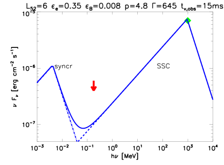
Figure 1: Modeling of the high energy emission during interval II in the IS scenario (Guetta & Granot, 2003). The red arrow marks the level of BAT upper-limits (see e.g. De Pasquale et al., 2010) while the green diamond marks the level of the flux observed by the LAT around 1 GeV (see Fig. 2 in Abdo et al., 2009b).

4 Synchrotron emission from the ES

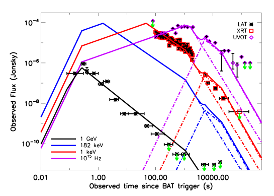
Figure 2: GRB 090510 broad-band modeling in the synchrotron ES scenario. Data are taken from the light curves in Fig. 1 of De Pasquale et al. (2010), where the mean flux measured in each energy range for the different instruments (Fermi/LAT, Swift/XRT and Swift/UVOT) has been rescaled to give the measured flux at each specific frequency (1 GeV, 1 keV and $10^{15}$ Hz). This is done by requiring at 100 s the specific flux value reported in the SED plotted in Fig. 2 of De Pasquale et al. (2010). The black, red, and purple solid lines represent the model predictions at 1 GeV, 1 keV and $10^{15}$ Hz, respectively. Parameters are set as follows, for the narrow and wide jet components (dash-dotted lines), respectively: $\epsilon_{e}=0.1$, $\epsilon_{B}=3\times 10^{-3}$, $n=10^{-6}$, $\Gamma_{0,n}=10^{4}$, $E_{iso,n}=3.7\times 10^{53}$ erg, $p_{n}=2.3$, $\theta_{j,n}=0.12^{\circ}$, $\Gamma_{0,w}=220$, $E_{iso,w}=1.5\times 10^{53}$ erg, $p_{w}=2.5$, $\theta_{j,w}=0.43^{\circ}$. The blue lines represent the contribution of the narrow and wide jet components at the middle of the BAT energy band; throughout the evolution this is below the data/upper-limits reported in De Pasquale et al. (2010), in agreement with our hypothesis that the emission observed in the GBM/BAT/MCAL energy range should be due to IS rather than to ES.

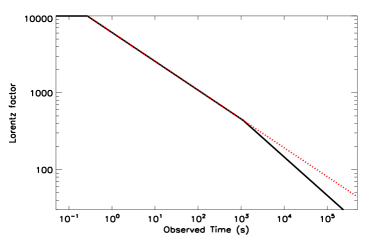
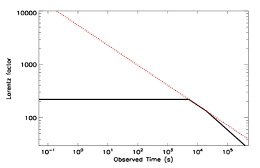
Figure 3: Temporal evolution (black lines) of the Lorentz factor for the narrow (left panel) and wide (right panel) jet components. The red-dotted lines are plotted for comparison, and correspond to the standard evolution $\Gamma\propto t^{-3/8}$ for an adiabatic fireball expanding in a uniform medium (e.g. Sari et al., 1998). The initial values $\Gamma_{0}$ are set to be $10^{4}$ and $220$, for the narrow and wide jet components, respectively. After $t_{j}$, which is set to be $\sim 1000$ s for the narrow jet (corresponding to $\theta_{j}\sim 0.1^{\circ}$), and $\sim 2\times 10^{4}$ s for the wide jet (corresponding to $\theta_{j}\sim 0.4^{\circ}$), the Lorentz factor is evolved following a temporal scaling of $\Gamma\propto t^{-1/2}$ (e.g. Peng et al., 2005) .

In this section, we test whether the high-energy emission observed by the Fermi/LAT, and the optical-to-X-ray emission observed later on by Swift, can be explained as ES afterglow, while the emission in the Fermi/GBM, AGILE/MCAL and Swift/BAT is due to IS. In this way, one can easily account for both the high temporal variability observed during the prompt burst (as related to IS), and for the delayed onset of the high-energy emission (as related to the onset of the afterglow). This hypothesis, first proposed by Ghirlanda et al. (2010) on the basis of the temporal behavior of the high energy tail observed in the LAT up to 100 s after the burst, was then confirmed as a viable possibility by De Pasquale et al. (2010) performing a broad-band analysis based on Swift BAT, XRT, UVOT, Fermi GBM, and LAT data. The striking feature of the broad-band observations is that the spectral energy distribution of the emission observed at 100 s is consistent with a single spectral component (De Pasquale et al., 2010). Here we assume the most natural hypothesis of it being simply the synchrotron high energy tail.

De Pasquale et al. (2010) have suggested that, within the ES model, the peak observed around $\sim 0.2-0.3$ s after the BAT trigger in the Fermi/LAT light curve of the extended tail could be associated with the fireball deceleration time, while the peak observed in the optical range could be due to the synchrotron peak frequency $\nu_{m}$ crossing the band. In light of these considerations, we have modeled the synchrotron emission from the ES to test if a reasonable set of parameters does indeed exist to provide such an explanation. To this end, we adopt the prescriptions by Sari et al. (1998) for the peak flux $f_{m}$, the injection frequency $\nu_{m}$, and the cooling frequency $\nu_{c}$:

$$f_{m}\propto\Gamma^{8}t^{3}_{obs}n^{3/2}\epsilon_{B}^{1/2}(1+z)^{-2}\,;$$ (27)

$$\nu_{m}\propto\left(\frac{p-2}{p-1}\right)^{2}\Gamma^{4}\epsilon_{e}^{2}\epsilon_{B}^{1/2}n^{1/2}(1+z)^{-1}\,;$$ (28)

$$\nu_{c}\propto\Gamma^{-4}t^{-2}_{obs}n^{-3/2}\epsilon_{b}^{-3/2}(1+z)\,.$$ (29)

We further rescale the expression for $\nu_{c}$ by a factor of $Y^{-2}$, to account for the effect of SSC losses on the synchrotron spectrum. Here $Y$ is the Compton parameter and is defined as follows (Sari & Esin, 2001):

$$Y = max\left[1,\sqrt{\frac{\epsilon_{e}}{\epsilon_{B}}}\right]~{}~{}~{}~{}{\rm in~{}fast~{}cooling}\,;$$ (30)

$$Y = max\left[1,\left(\frac{\epsilon_{e}}{\epsilon_{B}}\right)^{1/(4-p)}\left(\frac{\nu_{c}}{\nu_{m}}\right)^{-(p-2)/2(4-p)}\right]~{}~{}~{}~{}{\rm in~{}slow~{}cooling}\,,$$ (31)

where $\nu_{c}$ is the non-rescaled value of the cooling frequency, as in Sari et al. (1998) and Eq. (29). To model the behavior of the high-energy tail, we consider the whole evolution of the Lorentz factor $\Gamma$ of the shell, using an approximate sharp transition from the coasting phase, when

$$\Gamma\sim\Gamma_{0},$$ (32)

to the deceleration phase, when (e.g. Sari et al., 1998)

$$\Gamma(t_{obs})=\Gamma_{0}(t_{obs}/t_{dec})^{-3/8}\,.$$ (33)

Here $t_{dec}$ is the deceleration time in the observer’s frame, given by (Sari & Piran, 1999)

$$t_{dec}=\left(\frac{3E_{iso}}{32\pi\Gamma_{0}^{8}nm_{p}c^{5}}\right)^{1/3}(1+z)\,,$$ (34)

where $m_{p}$ is the proton mass.

In Fig. 2 we show what we obtain for the parameter choice $\Gamma_{0}=10^{4}$, $n=10^{-6}$, $\epsilon_{B}=3\times 10^{-3}$, $\epsilon_{e}=0.1$, $E_{iso}=3.7\times 10^{53}$ erg. These values are consistent with the results by Kumar & Barniol Duran (2009), in which the GeV light curve was modeled starting at $\sim 1$ s after the BAT trigger, while here we are modeling also its peak around 0.2-0.3 s. The high value of the Lorentz factor is required to have $t_{dec}\sim 0.3$ s, so as to explain the peak observed in the LAT light curve. We also note that while the very low density value is still consistent with those that can be expected around short GRBs in the coalescing binary progenitor scenario (see e.g. Belczynski et al., 2006), the isotropic energy is much higher (though comparable to the one derived from the fluence observed in the LAT, see Abdo et al. (2009b)).

In the hypothesis that the steepening observed in the XRT light curve is due to a jet break, we have further evolved the Lorentz factor as $\Gamma\propto(t_{obs}/t_{j})^{-1/2}$ (see e.g. Peng et al., 2005, and Fig. 3), finding that $t_{j}\sim 1000$ s in good agreement with the data. Using the relation (e.g. Rhoads, 1997)

$$\Gamma(t_{j})=1/\theta_{j}\,,$$ (35)

and considering Eq. (33), we can constrain the jet opening angle to be

$$\theta_{j}=\Gamma_{0}^{-1}(10^{3}~{}{\rm s}/0.3~{}{\rm s})^{3/8}\sim 0.1^{\circ}\,.$$ (36)

The energy in the jet is thus

$$E_{j}=(\theta_{j}^{2}/2)E_{iso}\sim 7\times 10^{47}~{}{\rm erg}\,,$$ (37)

which is more easily explained in a binary merger model.

We note, however, that after the X-ray break the optical flux decreases with a slope shallower than the X-ray one. De Pasquale et al. (2010) and Kumar & Barniol Duran (2009) have suggested that this may be explained by a jet break made shallower from the passage of $\nu_{m}$ through the optical band. With our choice of parameters, $\nu_{m}$ is crossing the optical band around the jet break time, and the light curve decay is still too steep (at least using our simple approximation of the Lorentz factor evolution). We therefore test the alternative hypothesis of a two-component jet, with a narrow jet component explaining the early time emission, and a wider component contributing at late times to explain the excess observed in the optical band. For example, Peng et al. (2005) considered such a model to explain the optical light curve of GRB 030329. By assuming for both jet components the same $\epsilon_{e}$, $\epsilon_{B}$ and $p$, Peng et al. (2005) found that the addition of a wider, slower component with $\Gamma_{0,w}\sim(1/10)\Gamma_{0,n}$ and $E_{j,w}\sim 4E_{j,n}$ could explain the late-time optical excess observed in the light curve. A structured jet model has also been invoked in other cases (e.g. Racusin et al., 2008) to explain chromatic jet breaks.

In light of these considerations, we have attempted to explain the optical excess observed in the case of GRB 090510 after $t_{obs}\sim 10^{3}$ s by adding the contribution of a wider jet component. We find that the choice $E_{w,iso}=1.5\times 10^{53}$, $\Gamma_{0,w}\sim(1/45)\Gamma_{0,n}=220$, $\theta_{j,w}=0.4^{\circ}$, and $p=2.5$ (with the other parameters left unchanged) can account for the excess observed in the optical, with little contribution in the X-rays (see Fig. 2 and Fig. 3). This choice also implies $E_{j,w}\sim 6E_{j,n}$. The chosen value of $p=2.5$ is larger than the one adopted for the narrow component. This is motivated by the fact that the X-ray decay observed before $10^{3}$ s, dominated by the narrow component, is shallower than the one observed after $10^{3}$ s in the optical band ($\delta=-1.13^{+0.17}_{-0.09}$), which we model as the emission from the wider component. With $p=2.5$, for $\nu_{m}<\nu_{opt}<\nu_{c}$ one gets a predicted value of the temporal decay index of $-3/4(p-1)\sim-1.12$, in agreement with the observed one within the uncertainties. Incidentally, we note that for the case of GRB 080319B, Racusin et al. (2008) obtained different $p$ values for the narrow- and wide-jet components, as we are finding here.

We finally test whether, for our choice of parameters, the contribution of SSC emission to the observed flux is indeed negligible (as suggested by the SED at 100 s being consistent with a single spectral component; see De Pasquale et al. (2010)). The peak flux of the SSC component, in the Thomson limit, is related to the synchrotron one by $f^{IC}_{m}\sim 10^{-6}n(R/10^{19}{\rm cm})f_{m}$ (Sari & Esin, 2001). In our case, the peak of the synchrotron component is constrained to fit the optical flux measured by the UVOT, which is about $10^{-4}$ Jy (see Fig. 2). This means that for $n=10^{-6}$, the SSC component has a flux level below $10^{-16}$ Jy at all energies throughout the evolution, so that its contribution to the light curves plotted in Fig. 2 is completely negligible.

5 Conclusion

We have analyzed GRB 090510 in the context of the synchrotron IS and ES scenarios. We first attempted to explain the soft-to-hard spectral evolution associated to the delayed onset of a GeV tail with the hypothesis that both the prompt burst and the high-energy tail originate from synchrotron emission of electrons accelerated by IS. Considerations of the compactness of the source lead us to conclude that the high-energy tail should be produced in IS developing in a late-emitted shell, characterized by a Lorentz factor of the order of $\Gamma\sim 700$, greater than the one generating the prompt burst ($\Gamma\sim 200$). However, this condition on the Lorentz factor implies a hard-to-soft evolution of the peak frequency of the IS synchrotron component, which does not agree with the observed soft-to-hard evolution.

Given the difficulties of explaining the prompt and delayed high energy emission with a single mechanism (synchrotron emission from IS), we then tested two double-component scenarios. In the first, the emission observed during interval I is explained as synchrotron emission from IS, while the high-energy tail observed in interval II is explained as SSC emission from IS. In the second scenario, the high energy emission observed by the LAT is decoupled from the prompt burst, and has an external shock origin. This last scenario has the advantage of explaining in a simple way the smooth temporal behavior of the high-energy tail, up to 100 s after the burst, and the consistency of the broad-band SED observed at 100 s with a single spectral component. In the ES scenario, we show that a reasonable set of parameters does indeed exist to explain the optical-to-GeV observations of this burst, despite a high Lorentz factor being required to have the fireball entering the deceleration phase as early as $t_{obs}\sim 0.3$ s (when the emission in the LAT is observed to peak). The ES scenario thus seems to account more naturally for the observations, even if a more detailed modeling of the late-time chromatic break is required. We have suggested that a structured jet may indeed be a viable explanation of such a chromatic feature.

In conclusion, we stress that the high Lorentz factor implied by the ES scenario has some relevant consequences in relation to the physics of the central engine. The commonly accepted fireball model invokes a series of shells expanding outward with Lorentz factor of the order of a few hundred, where IS first generate the prompt emission, and then, with the merged shell continuing to expand outward toward the external medium, an ES generates the afterglow. If, on the other hand, the high-energy tail is attributed to the ES emission, this implies that the source emits first a very fast shell, which impacts on the external medium creating an early afterglow, plus a series of slower shells that catch up with each other generating the prompt $\gamma$-ray emission. At the end of the IS phase, the merged, slower shell (with a more typical Lorentz factor of the order of a few hundred), would also decelerate and eventually generate an afterglow by interaction with the external medium. In this respect, we note that the additional component required to explain the shallow decay observed at late times in the optical band could be related to the ES generated by such a slower shell.

References

- Abdo et al. (2009a) Abdo, A. A., et al. 2009a, ApJ, 707, 580
- Abdo et al. (2009b) —. 2009b, Nature, 331, 462
- Asano et al. (2009) Asano, K., Guiriec, S., & Mészáros, P. 2009, ApJL, 705, L191
- Band et al. (1993) Band, D., et al. 1993, ApJ, 413, 281
- Belczynski et al. (2006) Belczynski, K., et al. 2006, ApJ, 648, 1110
- Corsi et al. (2009) Corsi, A., et al. 2009, A&A submitted to, ArXiv e-prints 0905.1513
- Costa et al. (1997) Costa, E., et al. 1997, Nature, 387, 783
- De Pasquale et al. (2010) De Pasquale, M., et al. 2010, ApJ, 709, L146
- Gao et al. (2009) Gao, W., Mao, J., Xu, D., & Fan, Y. 2009, ApJL, 706, L33
- Ghirlanda et al. (2010) Ghirlanda, G., et al. 2010, A&A, 510, L7
- Ghisellini et al. (1988) Ghisellini, G., Guilbert, P. W., & Svensson, R. 1988, ApJL, 334, L5
- Giuliani et al. (2010) Giuliani, A., et al. 2010, ApJ, 708, L84
- Guetta & Granot (2003) Guetta, D., & Granot, J. 2003, ApJ, 585, 885
- Guetta et al. (2001) Guetta, D., Spada, M., & Waxman, E. 2001, ApJ, 557, 399
- Hoversten et al. (2009) Hoversten, E. A., et al. 2009, GCN report, 218
- Kaneko et al. (2006) Kaneko, Y., Preece, R. D., Briggs, M. S., Paciesas, W. S., Meegan, C. A., & Band, D. L. 2006, ApJS, 166, 298
- Kouvelioutou et al. (1993) Kouvelioutou, C., et al. 1993, ApJ, 413, 101
- Kumar & Barniol Duran (2009) Kumar, P., & Barniol Duran, R. 2009, MNRAS submitted to, ArXiv e-prints 0910.5726
- Lithwick & Sari (2001) Lithwick, Y., & Sari, R. 2001, ApJ, 555, 540
- Meszaros & Rees (2000) Meszaros, P., & Rees, M. 2000, ApJ, 530, 292
- Meszaros & Rees (1992) Meszaros, P., & Rees, M. J. 1992, MNRAS, 257, 29
- Mészáros & Rees (1993) Mészáros, P., & Rees, M. J. 1993, ApJ, 405, 278
- Ohno et al. (2009) Ohno, M., et al. 2009, GCN, 9334
- Omodei (2008) Omodei, N. 2008, GCN, 8407
- Pe’er & Waxman (2004) Pe’er, A., & Waxman, E. 2004, ApJ, 613, 448
- Peng et al. (2005) Peng, F., Königl, A., & Granot, J. 2005, ApJ, 626, 966
- Piran (1999) Piran, T. 1999, Phys. Rep., 314, 575
- Racusin et al. (2008) Racusin, J. L., et al. 2008, Nature, 455, 183
- Ray et al. (2009) Ray, A., et al. 2009, GCN, 9353
- Rees & Mészáros (2005) Rees, M. J., & Mészáros, P. 2005, ApJ, 628, 847
- Rhoads (1997) Rhoads, J. E. 1997, ApJL, 487, L1
- Sari & Esin (2001) Sari, R., & Esin, A. A. 2001, ApJ, 548, 787
- Sari & Piran (1997) Sari, R., & Piran, T. 1997, MNRAS, 287, 110
- Sari & Piran (1999) —. 1999, ApJ, 520, 641
- Sari et al. (1998) Sari, R., Piran, T., & Narayan, R. 1998, ApJ, 497, L17
- Toma et al. (2010) Toma, K., Wu, X., & Meszaros, P. 2010, ArXiv e-prints 1002.2634
- Ukwatta et al. (2009) Ukwatta , T. N., et al. 2009, CGN, 9337
- Zou et al. (2009) Zou, Y.-C., Fan, Y.-Z., & Piran, T. 2009, MNRAS, 396, 1163