Designing fuzzy rule based classifier using self-organizing feature map for analysis of multispectral satellite images

Abstract

We propose a novel scheme for designing fuzzy rule based classifier. An SOFM based method is used for generating a set of prototypes which is used to generate a set of fuzzy rules. Each rule represents a region in the feature space that we call the context of the rule. The rules are tuned with respect to their context. We justified that the reasoning scheme may be different in different context leading to context sensitive inferencing. To realize context sensitive inferencing we used a softmin operator with a tunable parameter. The proposed scheme is tested on several multispectral satellite image data sets and the performance is found to be much better than the results reported in the literature.

1 Introduction

A classifier [1] can be defined as any function ${\cal D}:\Re^{p}\rightarrow N_{c}$, where $N_{c}=\{{\bf e}_{i}\mid i=1,...,c,{\bf e}_{i}\in\Re^{c}\}$ is the set of label vectors and $c$ is the number of classes. Given any feature vector ${\bf x}\in\Re^{p}$, it produces a label vector in $\Re^{c}$. If ${\cal D}$ is a crisp classifier, ${\bf e}_{i}$s are basis vectors with components $e_{ij}=0\forall i\neq j$ and $e_{ii}=1$. If ${\cal D}$ is a fuzzy classifier then $e_{ij}\geq 0$ and $\sum_{j=1}^{c}e_{ij}=1$. Designing a classifier involves finding a good ${\cal D}$.

Although Bayes’ classifier is optimal [1] it requires statistical knowledge of the sample set in terms of prior probabilities and class conditional densities, which are almost never available in practical cases. Usually no knowledge of the underlying distribution is available except whatever can be inferred from samples. In such a case the classifier has to rely on a set of labeled samples $X=\{({\bf x}_{i},{\bf l}_{i}\mid i=1,...,n,{\bf x}_{i}\in\Re^{p},{\bf l}_{i}\in N_{c})\}$, where ${\bf l}_{i}$ is the label vector associated with the training vector ${\bf x}_{i}$. The training samples are assumed to be a true representative of the data to be classified. Nonparametric classification schemes do not use any parametric model [2, 3] but utilize the training samples in a suitable training procedure to model the distribution of the input data and use the model to infer about the class membership of unknown data points.

For example, a crisp $k$-NN classifier uses the whole set of training samples to infer the class membership of an unknown input vector ${\bf x}\in\Re^{p}$ using the following rule:$\diamond$ Find the set of $k$ samples $\{({\bf x}_{i},{\bf l}_{i})\}\in X$ closest to the sample ${\bf x}$ $\diamond$ Assign the sample ${\bf x}$ to the class from which majority of $k$ closest neighbors has come.

On the other hand, a prototype based classifier approximates the distribution of the training data through a set of prototypes $V=\{{\bf v}_{i},{\bf l}_{i}\mid i=1,...,\hat{c}\geq c,{\bf v}_{i}\in\Re^{p},{\bf l}_{i}\in N_{c}\}$, and classifies a vector ${\bf x}\in\Re^{p}$ as follows.

Decide ${\bf x}\in$ class $i\Leftrightarrow{\cal D}_{V,\delta}({\bf x})={\bf l}_{i}\Leftrightarrow\delta({\bf x},{\bf v}_{i})\leq\delta({\bf x},{\bf v}_{j})\forall i\neq j.$

where $\delta$ is usually the Euclidean distance function.

In recent times fuzzy rule based classifiers [4, 5, 6, 7] have attracted attention of many researchers due to their several attractive features compared to more traditional distance based classifiers. At the conceptual level their working is closer in spirit to human reasoning. At the practical level they can be used very easily to handle several problematic situations. For example, detection of outliers can be done using small firing strengths of the rules, highly overlapped regions can be detected by high firing strength for rules from more than one class. Most interestingly, the problem of high variation in the variances of different features, which often degrades the performance of a distance based classifier substantially, can be handled naturally by fuzzy rules due to the atomic nature of the antecedent clauses. It may be noted that the use of Mahalanobis distance can handle, to some extent, the problem associated with variation in variances of different features. However, if the training data from a class are divided into several clusters with different distributions, then Mahalanobis distance may not be very effective, but fuzzy rules will be able to model such class structures in a natural manner.

A fuzzy rule based classifier consists of a set of fuzzy rules of the form:$R_{i}:$ If $x_{1}$ is $A_{i1}$ AND $x_{2}$ is $A_{i2}$ AND $\cdots$ AND $x_{p}$ is $A_{ip}$ then class is $j$.Here $A_{ik}$ is a fuzzy set used in the i-th rule and defined on the domain of $x_{k}$, i.e., on the universe of the k-th feature.

When a sample data point ${\bf x}\in\Re^{p}$ is presented to the system for classification, the fuzzy rules fire to produce outputs. The magnitude of the outputs ( also known as firing strengths) are used for deciding the class membership of the sample data ${\bf x}$.

For designing a fuzzy rule based classifier there are three issues that need to be addressed:

$I_{1}$ : How many rules are needed?$I_{2}$ : How to generate the rules? $I_{3}$ : How to use the rules to decide a class?

The simplest way of tackling the above issues is to take the help of a domain expert and create the fuzzy rules to represent his/her domain knowledge. But in a typical pattern classification problem, such domain knowledge is usually not available. So a scheme is needed for designing fuzzy rule based classifier based on the training samples.

In this paper we describe a comprehensive scheme for designing fuzzy rule based classifiers. The scheme takes care of all the three issues mentioned above. This is a multi-stage scheme. In the first stage a set of labeled prototypes representing the distribution of the training data is generated using a Self-organizing Feature Map (SOFM) [11, 12, 13]. The algorithm employs a combination of unsupervised and supervised clustering of the training data to generate an adequate number of prototypes representing the overall as well as class-specific distribution of the training data. Then each of these prototypes is converted to a fuzzy rule of the form described above. Thus, each of the fuzzy rules represents a region, may be overlapped, in the feature space. We call this region the context of the rule. Note that, throughout this paper the word “context” is used to mean a region in the feature space, not pixels in the neighborhood of another pixel in an image.

Next we develop a tuning algorithm for the fuzzy rules that fine-tunes the peaks as well as the spreads of the fuzzy sets associated with the rules. We call this the context tuning stage. However, the exact implementation of the tuning algorithm is dependent on the conjunction operator used to represent the AND connective in the antecedent part of the rules. Here we derive tuning algorithms for two different conjunction operators, namely the product and the softmin. The tuned rules are used to classify the unknown samples based on the firing strengths of the rules. A test sample is classified to the class of the rule generating the highest firing strength.

The softmin operator, based on the value of a parameter can approximate a whole family of operators including min, average and max. This raises the possibility of using a set of rules where each rule is free to use a different conjunction operator depending on the context it operates on. This is known as context-sensitive reasoning. Here, depending on the context the reasoning scheme may change. To realize this possibility we also develop an algorithm for tuning the parameters of the softmin operators on a per-rule basis. The schemes using the same conjunction operator (reasoning scheme) for all rules will be called context-free reasoning in this paper.

Classification of multispectral satellite images is a very important field of application of pattern recognition techniques. Currently huge amount of information about the earth is routinely being generated by the satellite-based sensors. This information is often available in the form of multispectral images produced by a set of sensors operating in different spectral regions. A sensor operating in certain spectral region might be more sensitive to certain classes of objects than the others. Hence, to develop a good analysis system it is necessary to use data available from as many sensors as possible. This requirement led to development of numerous techniques for data fusion and classification. To name a few, statistical methods [14, 15], Dempster-Shafer theory [16], neural networks [15, 17, 18, 19] etc.

Numerous fuzzy classification techniques have been developed by many researchers to solve problems in various fields. A comprehensive account of such works can be found in [4, 5, 7]. Many references are available on the use of different fuzzy methodologies for land cover classification from multispectral satellite images. For example, [8, 9] uses fuzzy $c$-means algorithm [4], Kumar et al. [25] applied fuzzy integral method. Fuzzy rule base has also been used for classification by many researchers [5, 6] for diverse fields of application. Fuzzy rules are attractive because they are interpretable and can provide an analyst a deeper insight into the problem. Not many attempts have been made to use fuzzy rule based systems for land cover analysis. In a recent paper Bárdossy and Samaniego [10] have proposed a scheme for developing a fuzzy rulebased classifier for analysis of multispectral images. They employed simulated annealing for optimizing the performance of a randomly selected initial set of rules. In the present paper we propose a prototype-based fuzzy rule generation approach [5], where the number of prototypes (hence the number of rules) depends on the complexity of the training data.

Though our scheme is applicable to any pattern recognition task using object data, we have chosen to test our scheme on satellite images because context sensitive inferencing could be very effective for them. Analysis of satellite images has many important applications such as prediction of storm and rainfall, assessment of natural resources, estimation of crop yields, assessment of natural disasters, and land cover classification. In this paper we focus on land cover classification from multi-spectral satellite images. We consider a set of independent detectors of a sensor, operating in different spectral bands and producing homogeneous data (i.e., same type of information, namely pixel values). The weakly coupled fused data [20] consist of one data vector for each pixel, data from each detector contributing to one dimension of the data vectors. We use the weakly coupled data along with the ground truth to train a classifier. We use images from two types of sensors, a 7-channel image and a 4-channel image produced by a Landsat Multispectral Scanner [24] and a Thematic Mapper respectively [7].

Details of the scheme and the experimental results are described in the following sections. Section 2 covers the method of generating the prototypes, the method for converting the prototypes into fuzzy rules and the context tuning algorithms. Section 3 contains the description of context sensitive reasoning methods. The experimental results and the discussions are presented in section 4. Section 5 concludes the paper.

2 Designing of the Fuzzy Rule based Classifiers

The proposed scheme has several stages. We use Kohonen’s Self-Organizing Feature Map (SOFM)[11] to obtain a set of prototypes. For the sake of completeness we provide a brief description of SOFM.

2.1 Kohonen’s SOFM algorithm

The self-organizing feature map is an algorithmic transformation denoted here by $A^{D}_{SOFM}:\Re^{p}\rightarrow V(\Re^{q})$ that is often advocated for visualization of metric-topological relationships and distributional density properties of feature vectors (signals) $X=\{{\bf x}_{1},...,{\bf x}_{N}\}$ in $\Re^{p}$. SOFM is implemented through a two-layered neural architecture that is believed to be similar in some ways to the biological neural network. The input layer is a fan-out layer and the output layer is a competitive layer. Each node in the input layer is connected to all nodes in the competitive layer.

The visual display produced by $A^{D}_{SOFM}$ presumably helps one form hypotheses about topological structure in $X$. In principle $X$ can be transformed onto a display lattice in $\Re^{q}$ for any $q$; in practice, visual display can be made only for $q\leq 3$ and are usually made on a linear or planar configuration arranged as a rectangular or hexagonal lattice. Here we explain architecture and training procedure of SOFM using ($m\times n$) display or output nodes.

Input vectors ${\bf x}\in\Re^{p}$ are distributed by a fan-out layer to each of the ($m\times n$) output nodes in the competitive layer. Each node in this layer has a weight vector (prototype) ${\bf w}_{ij}$ attached to it. We let $O_{p}=\{{\bf w}_{ij}\}\subset\Re^{p}$ denote the set of ${\em m}\times{\em n}$ weight vectors. $O_{p}$ is (logically) connected to a display grid $O_{2}\subset V(\Re^{2})$. ($i,j$) in the index set $\{1,2,\ldots,m\}\times\{1,2,\ldots,n\}$ is the logical address of the cell. There is a one-to-one correspondence between the $m\times n$ p-vectors ${\bf w}_{ij}$ and the $m\times n$ cells ($\{i,j\}$),i.e., $O_{p}\longleftrightarrow O_{2}$.

SOFM usually begins with a random initialization of the weight vectors ${\bf w}_{ij}$. For notational clarity we suppress the double subscripts. Now let ${\bf x}\in\Re^{p}$ enter the network and let $t$ denote the current iteration number. Find ${\bf w}_{r,t-1}$, that best matches ${\bf x}$ in the sense of minimum Euclidean distance in $\Re^{p}$. This vector has a (logical) “image” which is the cell in $O_{2}$ with subscript $r$. Next a topological (spatial) neighborhood $N_{r}(t)$ centered at $r$ is defined in $O_{2}$, and its display cell neighbors are located. For example, $3\times 3$ window, $N(r)$, centered at $r$ corresponds to nine prototypes in $\Re^{p}$. Finally, ${\bf w}_{r,t-1}$ and the other weight vectors associated with cells in the spatial neighborhood $N_{t}(r)$ are updated using the rule

$${\bf w}_{i,t}={\bf w}_{i,t-1}+h_{ri}(t)({\bf x}-{\bf w}_{i,t-1}).$$ (1)

Here $r$ is the index of the “winner” prototype

$$r=\underbrace{arg\ min}_{i}\{\|{\bf x}-{\bf w}_{i,t-1}\|\}$$ (2)

and $\|*\|$ is the Euclidean norm on $\Re^{p}$. The function $h_{ri}(t)$ which expresses the strength of interaction between cells $r$ and $i$ in $O_{2}$, usually decreases with $t$, and for a fixed $t$ it decreases as the distance (in $O_{2}$) from cell $r$ to cell $i$ increases. $h_{ri}(t)$ is usually expressed as the product of a learning parameter $\alpha_{t}$ and a lateral feedback function $g_{t}(dist(r,i))$. A common choice for $g_{t}$ is $g_{t}(dist(r,i))=\exp^{-dist^{2}(r,i)/\sigma^{2}_{t}}$. $\alpha_{t}$ and $\sigma_{t}$ both decrease with time $t$. The topological neighborhood $N_{t}(r)$ also decreases with time. This scheme when repeated long enough, usually preserves spatial order in the sense that weight vectors which are metrically close in $\Re^{p}$ generally have, at termination of the learning procedure, visually close images on the display lattice.

2.2 Generation of Prototypes

We use a 1-D SOFM, but the algorithm can be extended to 2-D SOFM also. First we train a one-dimensional SOFM using the training data, of course, without using the class information of the input data. We start the SOFM with c nodes where $c$ is the number of classes. We do so because the smallest number of rules that may be required is equal to the number of classes. At the end of the training the weight vector distribution of the SOFM reflects the distribution of the input data. These unlabeled prototypes are then labeled using class information. For each of $N$ input feature vectors we identify the prototype closest to it, i.e., the winner node. Since no class information is used during the training, some prototypes may become the winner for data from more than one class. For each prototype ${\bf v}_{i}$ we compute a score $D_{ij}$, which is the number of data points from class $j$ to which ${\bf v}_{i}$ is the closest prototype. If $D_{ij}$ is 0 for all $j$ for a prototype ${\bf v}_{i}$ then we reject it. For the remaining prototypes the class label $C_{i}$ of the prototype ${\bf v}_{i}$ is determined as

$$C_{i}=\underbrace{arg\max}_{j}D_{ij}.$$ (3)

The scheme assigns a label to each of the $c$ prototypes, but such a set of prototypes may not classify the data satisfactorily. For example, from (3) it is clear that $\sum_{j\neq i}D_{ij}$ data points will be wrongly classified by the prototype ${\bf v}_{i}$. Hence we need further refinement of the initial set of prototypes $V_{0}=\{{\bf v}_{10},{\bf v}_{20},...,{\bf v}_{c0}\}\subset\Re^{p}$.

We use the prototype refinement scheme described in [12, 13]. The basic idea behind this refinement algorithm is that a useful prototype, ${\bf v}_{i}$ should satisfy two criteria:(i) It should represent adequate number of points, i.e., $W_{i}=\sum_{j=1}^{c}D_{ij}$ should be high.(ii) Only one of the classes, say class $k$, should be strongly represented by ${\bf v}_{i}$, i.e., $D_{ik}$ should be high and $D_{ij},\forall j\neq k$ should be low.

If condition (i) is not satisfied ${\bf v}_{i}$ is deleted and depending on the values of $D_{ij}$ prototypes are split and merged. Finally, the set of prototypes are again refined by SOFM algorithm with winner-only update strategy. After a few iterations this algorithm produces a set of adequate number of prototypes that represents the training data much better than the initial one. For details the readers are referred to [12, 13].

Now we use these prototypes to generate fuzzy rules that we describe next.

2.3 Designing fuzzy rulebased classifiers

A prototype (representing a cluster of points) ${\bf v}_{i}$ for class $k$ can be translated into a fuzzy rule of the form :

$R_{i}$: If ${\bf x}$ is CLOSE TO ${\bf v}_{i}$ then the class is $k$.

Where the fuzzy set “CLOSE TO” can be represented by a multidimensional membership function such as

$$\mu_{CLOSETO}({\bf x})=\exp^{-\frac{||{\bf x}-{\bf v}_{i}||^{2}}{{\sigma_{i}}^{2}}},$$

where $\sigma_{i}>0$ is a constant. This is equivalent to using prototypes with hyperspherical zones of influence centered at ${\bf v}_{i}$s. The 1-MSP (most similar prototype) classifier uses such membership values and it has been studied in [13]. Such a classifier does not perform quite well when different features have considerably different variances.

To overcome this shortcoming, “${\bf x}$ is CLOSE TO ${\bf v}_{i}$” can be written as a conjunction of $p$ atomic clauses :

$x_{1}$ is CLOSE TO $v_{1}$ AND $\cdots$ AND $x_{p}$ is CLOSE TO $v_{p}$.

Such that the i-th rule $R_{i}$ representing one of the c classes takes the form

$R_{i}$ : $x_{1}$ is CLOSE TO $v_{i1}$ AND $\cdots$ AND $x_{p}$ is CLOSE TO $v_{ip}$ then class is $k$.

The fuzzy set CLOSE TO $v_{ij}$ can be modeled by triangular, trapezoidal or Gaussian membership function. In this investigation, we use the Gaussian membership function,

$$\mu_{ij}(x_{j};v_{ij},\sigma_{ij})=\exp{-{(x_{j}-v_{ij})}^{2}/{\sigma_{ij}}^{2}}.$$

Given a data point ${\bf x}$ with unknown class, we first find the firing strength of each rule. Let $\alpha_{i}({\bf x})$ denote the firing strength of the $i^{th}$ rule on a data point ${\bf x}$. The firing strength can be computed using any T-norm [5]. For example, using product the firing strength becomes

$$\alpha_{i}({\bf x})=\Pi_{j=1}^{j=p}\mu_{ij}(x_{j};v_{ij},\sigma_{ij}).$$

We then assign the point ${\bf x}$ to class $k$, if $\alpha_{r}=\max_{i}(\alpha_{i}({\bf x}))$ and the $r^{th}$ rule represents class $k$.

The performance of the classifier depends crucially on the adequacy of the number of rules used and proper choice of the fuzzy sets used in the antecedent part of the rules. In our case each fuzzy set is characterized by two parameters $v_{j}$ and $\sigma_{ij}$. The $v_{ij}$s of the rules can be initialized with the components of the final prototypes generated by our SOFM based algorithm, $V^{0}=V^{final}=\{{\bf v}_{1}^{final},\cdots,{\bf v}_{\hat{c}}^{final}\}$ $=\{{\bf v}_{1}^{0},\cdots,{\bf v}_{\hat{c}}^{0}\}$ where $v_{ij}^{0}=v_{ij}^{final}$ or they can be generated using any clustering algorithms like the fuzzy c-means [4] provided we know the required number of rules. A distinct advantage of using our SOFM based method is that it automatically decides on the required number of rules. The initial estimates of the $\sigma_{ij}$s are computed as follows.

For each prototype ${\bf v}_{i}^{0}$ in the set $V^{0}=\{{\bf v}_{i}^{0}\mid i=1,...,\hat{c},{\bf v}_{i}^{0}\in\Re^{p}\}$ let $X_{i}$ be the set of training data closest to ${\bf v}_{i}^{0}$. For each ${\bf v}_{i}^{0}$ the set

$$S_{i}=k_{w}\{\sigma_{ij}\mid j=1,...,p,\sigma_{ij}=(\sqrt{(}\sum_{{\bf x}_{k}\in X_{i}}(x_{kj}-v_{ij}^{0})^{2}))/|X_{i}|\}$$

is computed and associated with the prototype. $k_{w}>0$ is a constant parameter that controls the initial width of the membership function. Its value can have a significant impact on the classification performance for complicated data sets.

The initial rulebase $R^{0}$ thus obtained can be further fine tuned to achieve better performance. But the exact tuning algorithm depends on the conjunction operator (implementing AND operation for the antecedent part) used for computation of the firing strengths. We mentioned earlier that he firing strength can be calculated using any conjunction operator or T-norm [5]. Use of different T-norms result in different classifiers. The product and the minimum are among most popular T-norms used as conjunction operators. Using product the firing strength of r-th rule is computed as follows:

$$\alpha_{r}({\bf x})=\Pi_{j=1}^{j=p}\mu_{rj}(x_{j};v_{rj},\sigma_{rj}).$$

and the same when computed using the minimum is

$$\alpha_{r}=\min_{j}\{\mu_{rj}(x_{j};v_{rj},\sigma_{rj})\}.$$

It is much easier to formulate a calculus based tuning algorithm if product is used.

In the current study we design two different classifiers, one using product and the other using the Soft-min operator. We shall see that soft-min enables us to realize a novel context sensitive inferencing scheme.

2.3.1 Tuning of the Rule Base

Let ${\bf x}\in X$ be from class $c$ and ${R}_{c}$ be the rule from class $c$ giving the maximum firing strength $\alpha_{c}$ for ${\bf x}$. X is the training set. Also let ${R}_{\neg c}$ be the rule from the incorrect classes having the highest firing strength $\alpha_{\neg c}$ for ${\bf x}$.

We use the error function $E$,

$$E=\sum_{{\bf x}\in X}(1-\alpha_{c}+\alpha_{\neg c})^{2}.$$ (4)

This error function has been used by Chiu [21]. We minimize $E$ with respect to $v_{cj}$, $v_{\neg cj}$ and $\sigma_{cj}$, $\sigma_{\neg cj}$ of the two rules $R_{c}$ and $R_{\neg c}$. This will refine the rules with respect to their contexts.

Here the index $j$ corresponds to clause number in the corresponding rule, i.e., for the first antecedent clause $j=1$, for the second clause $j=2$ and so on. Next we give an algorithmic description of the rule refinement algorithm when product is used to compute the firing strength.

Rule refinement (context-tuning) algorithm:

Begin

Choose learning parameters $\eta_{m}$ and $\eta_{s}$.Choose a parameter reduction factor $0<\varepsilon<1$.Choose the maximum number of iteration $maxiter$.Compute the error $E_{0}$ for the initial rule base $R^{0}$. Compute the misclassification $M_{0}$ Corresponding to initial rule base $R^{0}$.

$t\leftarrow 1$While ($t\leq maxiter$) do         For each vector ${\bf x}\in X_{Tr}$ (The training set)                 Find the rules ${R}_{c}$ and ${R}_{\neg c}$ using $\alpha_{c}$ and $\alpha_{\neg c}$.                 Modify the parameters of rules ${R}_{c}$ and ${R}_{\neg c}$ as follows .

For $k=1$ to $p$ do                       (A) $v_{ck}^{new}=v_{ck}^{old}-\eta_{m}\frac{\partial E}{\partial v_{ck}^{old}}=v_{ck}^{old}+\eta_{m}(1-\alpha_{c}+\alpha_{\neg c})\frac{\alpha_{c}}{\sigma_{ck}^{old^{2}}}(x_{k}-v_{ck}^{old})$                      (B) $v_{\neg ck}^{new}=v_{\neg ck}^{old}-\eta_{m}\frac{\partial E}{\partial v_{\neg ck}^{old}}=v_{\neg ck}^{old}-\eta_{m}(1-\alpha_{c}+\alpha_{\neg c})\frac{\alpha_{\neg c}}{\sigma_{\neg ck}^{old^{2}}}(x_{k}-v_{\neg ck}^{old})$                      (C) $\sigma_{ck}^{new}=\sigma_{ck}^{old}-\eta_{s}\frac{\partial E}{\partial\sigma_{ck}^{old}}=\sigma_{ck}^{old}+\eta_{s}(1-\alpha_{c}+\alpha_{\neg c})\frac{\alpha_{c}}{\sigma_{ck}^{old^{3}}}(x_{k}-v_{ck}^{old})^{2}$                      (D) $\sigma_{\neg ck}^{new}=\sigma_{\neg ck}^{old}-\eta_{s}\frac{\partial E}{\partial\sigma_{\neg ck}^{old}}=\sigma_{\neg ck}^{old}-\eta_{s}(1-\alpha_{c}+\alpha_{\neg c})\frac{\alpha_{\neg c}}{\sigma_{\neg ck}^{old^{3}}}(x_{k}-v_{\neg ck}^{old})^{2}$                 End For          End For          Compute the error $E_{t}$ for the new rule base $R^{t}$.         Compute the misclassification $M_{t}$ for $R^{t}$.         If $M_{t}>M_{t-1}$ or $E_{t}>E_{t-1}$                  then                 $\eta_{m}\leftarrow(1-\varepsilon)\eta_{m}$                 $\eta_{s}\leftarrow(1-\varepsilon)\eta_{s}$                 $R^{t}\leftarrow R^{t-1}$                          /*If the error is increased, then possibly the learning coefficients are                           too large. So, decrease the learning coefficients, and retain $R_{t-1}$.*/         If $M_{t}=0$ or $E_{t}=0$                  then Stop.         $t\leftarrow t+1$End While

End

At the end of the rulebase tuning we get the final rulebase $R_{final}$ which is expected to give a very low error rate.

Since a Gaussian membership function is extended to infinity, for any data point all rules will be fired to some extent. In our implementation, if the firing strength is less than a threshold, $\epsilon$ $(\approx 0.01)$, then the rule is not assumed to be fired. Thus, under this situation, the rulebase extracted by the system may not be complete with respect to the training data. This can also happen when we use membership functions with triangular or trapezoidal shapes. This is not a limitation but a distinct advantage, although for the data sets we used, we did not encounter such a situation. If no rule is fired by a data point, then that point can be thought of as an outlier. If this happens for some test data, then that will indicate an observation not close enough to the training data and consequently no conclusion should be made about such test points.

Though product is a valid T-norm and has some attractive mathematical properties, its use is conceptually somewhat unattractive. To illustrate the point let us consider a rule having two atomic clauses in its antecedent. If the two clauses have truth values $a$ and $b$, then intuitively the antecedent is satisfied at least to the extent of $\min(a,b)$. However, if product is used as the conjunction operator, we always have $ab\leq\min(a,b)$. Thus we always under-determine the importance of the rule. This does not cause any problem for non-classifier fuzzy systems as defuzzification operator usually performs some kind of normalization with respect to the firing strength. But in classifier type applications a decision may appear to be taken with very low confidence, when actually it is not the case. For example, if each antecedent clause is satisfied to the extent 0.9 and there are 10 antecedent clauses, the firing strength becomes $0.9^{10}=0.3487$! Thus to avoid the use of the product and at the same time to be able to apply calculus to derive update rules we use a soft-min operator.

The soft-match of $n$ positive number $x_{1},x_{2},...,x_{n}$ is defined by

$$SM(x_{1},x_{2},...,x_{n},q)=\left\{\frac{(x_{1}^{q}+x_{2}^{q}+...+x_{n}^{q})}{n}\right\}^{1/q}.$$

where $q$ is any real number. $SM$ is known as an aggregation operator with upper bound of value 1 when $x_{i}\in[0,1]\forall i$. This operator is used by different authors [22, 23] for different purposes. It is easy to see that

$$\lim_{q\to\infty}SM(x_{1},x_{2},...,x_{n},q)=\max(x_{1},x_{2},...,x_{n})$$

and

$$\lim_{q\to-\infty}SM(x_{1},x_{2},...,x_{n},q)=\min(x_{1},x_{2},...,x_{n}).$$

Thus we define the softmin operator as the soft match operator with a sufficiently negative value of the parameter $q$. The firing strength of the r-th rule computed using softmin is

$$\alpha_{r}({\bf x})=\left\{\frac{\sum_{j=1}^{j=p}(\mu_{rj}(x_{j};v_{rj},\sigma_{rj}))^{q}}{p}\right\}^{1/q}.$$

In the current study we use $q=-10.0$.

Using the same error function as in the previous section we derive the rule update equations L, M, N, and O bellow.The tuning algorithm remains the same except equations A, B, C and D are replaced by L, M, N, and O respectively.

(L) $v_{ck}^{new}=v_{ck}^{old}-\eta_{m}\frac{\partial E}{\partial v_{ck}^{old}}=v_{ck}^{old}+\eta_{m}(1-\alpha_{c}+\alpha_{\neg c})\frac{\alpha_{c}}{\sum_{j=1}^{j=p}\mu_{cj}^{q}}\frac{\mu_{cj}^{q}}{\sigma_{ck}^{old^{2}}}(x_{k}-v_{ck}^{old})$(M) $v_{\neg ck}^{new}=v_{\neg ck}^{old}-\eta_{m}\frac{\partial E}{\partial v_{\neg ck}^{old}}=v_{\neg ck}^{old}-\eta_{m}(1-\alpha_{c}+\alpha_{\neg c})\frac{\alpha_{\neg c}}{\sum_{j=1}^{j=p}\mu_{\neg cj}^{q}}\frac{\mu_{\neg cj}^{q}}{\sigma_{\neg ck}^{old^{2}}}(x_{k}-v_{\neg ck}^{old})$(N) $\sigma_{ck}^{new}=\sigma_{ck}^{old}-\eta_{s}\frac{\partial E}{\partial\sigma_{ck}^{old}}=\sigma_{ck}^{old}+\eta_{s}(1-\alpha_{c}+\alpha_{\neg c})\frac{\alpha_{c}}{\sum_{j=1}^{j=p}\mu_{cj}^{q}}\frac{\mu_{cj}^{q}}{\sigma_{ck}^{old^{3}}}(x_{k}-v_{ck}^{old})^{2}$(O) $\sigma_{\neg ck}^{new}=\sigma_{\neg ck}^{old}-\eta_{s}\frac{\partial E}{\partial\sigma_{\neg ck}^{old}}=\sigma_{\neg ck}^{old}-\eta_{s}(1-\alpha_{c}+\alpha_{\neg c})\frac{\alpha_{\neg c}}{\sum_{j=1}^{j=p}\mu_{\neg cj}^{q}}\frac{\mu_{\neg cj}^{q}}{\sigma_{\neg ck}^{old^{3}}}(x_{k}-v_{\neg ck}^{old})^{2}$

The use of softmin is also consistent with our perception of AND connective in the antecedent parts of the fuzzy rules. Since for a reasonably big negative value (such as -10.0) of $q$ the softmin makes a very good approximation of min, when the trained system is used for testing/deployment, we can directly use min to reduce the computational overhead.

3 Context-Sensitive Inferencing

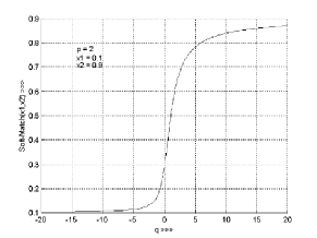
Figure 1: Plot of soft-match operator against $q$.

The use of softmin operator opens up a host of theoretical possibilities. The important fact to be noted is that the softmin operator is just one member of the family of aggregation operators generated by the soft-match operator for $q\in[-\infty,\infty]$. The family of operators covers a large spectrum from $minimum$ to $maximum$ including the $average$ (for $q=1$). Figure 1 shows that softmin varies from the minimum of its arguments to their maximum via the average.

In fuzzy rule based systems for pattern classification tasks, we use rules of the form

$R_{i}:$ If $x_{1}$ is $A_{i1}$ AND $\cdots$ AND $x_{p}$ is $A_{ip}$ then class is $j$,

Even if we use a tunable conjunction operator typically all rules in a system use the same conjunction operator. We can raise a fundamental question at this point. Is it really necessary to have the same conjunction operator for all rules in a system? It is very difficult to have a definite answer. A rule is considered to be a tool for reasoning in a small area of input feature space, each rule can be thought as a different context of reasoning. Thus drawing an analogy with the reasoning of human experts, we can recognize the possibility that within the same system there could be rules using different conjunction operators. Thus a system may contain some rules for which minimum is the appropriate conjunction operator while there could be others whose firing strength is larger than the minimum of the membership values of atomic propositions. There could even be some rules whose conjunction operator are closer in spirit to the maximum. This leads to a concept called context sensitive inferencing. Human being often do context sensitive inferencing. Depending on the cost involved with a decision an expert may adopt different level of conservatism in inferencing [23].

Thus while designing a scheme for rule extraction from the data, if the conjunction operator for each rule can also be learnt from the data, the resulting system is expected to achieve better performance.

In our present scheme we use the softmin as the conjunction operator. As mentioned above, it can act as different conjunction operators for different value of its parameter $q$. So we can calculate the firing strength for the $r^{th}$ rule $R_{r}$ as

$$\alpha_{r}({\bf x})=\left\{\frac{\sum_{j=1}^{j=p}(\mu_{rj}(x_{j};v_{rj},\sigma_{rj}))^{q_{r}}}{p}\right\}^{1/q_{r}}.$$

i.e., $q_{r}$ is the parameter for conjunction operator corresponding to the $r^{th}$ rule. Hence, the error function can be written as

$$E(q_{1},q_{2},\cdots q_{\mid R\mid})=\sum_{{\bf x}\in X}(1-\alpha_{c}+\alpha_{\neg c})^{2},$$ (5)

where $R$ is the set of rules. Now using gradient descent we can formulate an update scheme for $q_{i}$s in addition to $v_{ij}$ and $\sigma_{ij}$s for reducing the error function. The algorithm for tuning consequent operators is given bellow.

The conjunction operator refinement algorithm:

Begin

Choose learning parameter $\eta_{q}$.Choose a parameter reduction factor $0<\varepsilon<1$.Choose the maximum number of iteration $maxiter$.Compute the error $E_{0}$ for the initial rule base $R^{0}$.

$t\leftarrow 1$While ($t\leq maxiter$) do         For each vector ${\bf x}\in X$                 Find the rules ${R}_{c}$ and ${R}_{\neg c}$ using $\alpha_{c}$ and $\alpha_{\neg c}$.                 Modify the parameters $q_{c}$ and $q_{\neg c}$ of rules ${R}_{c}$ and ${R}_{\neg c}$ respectively as follows .

$q_{c}^{new}=q_{c}^{old}-\eta_{q}\frac{\partial E}{\partial q_{c}^{old}}=q_{c}^{old}+\eta_{q}(1-\alpha_{c}+\alpha_{\neg c})\frac{\alpha_{c}}{q_{c}}\left(\frac{\sum_{j=1}^{j=p}\mu_{cj}^{q_{c}}\ln\mu_{cj}}{\sum_{j=1}^{j=p}\mu_{cj}^{q_{c}}}-\ln\alpha_{c}\right)$

$q_{\neg c}^{new}=q_{\neg c}^{old}-\eta_{q}\frac{\partial E}{\partial q_{\neg c}^{old}}=q_{\neg c}^{old}+\eta_{q}(1-\alpha_{c}+\alpha_{\neg c})\frac{\alpha_{\neg c}}{q_{\neg c}}\left(\frac{\sum_{j=1}^{j=p}\mu_{\neg cj}^{q_{\neg c}}\ln\mu_{\neg cj}}{\sum_{j=1}^{j=p}\mu_{\neg cj}^{q_{\neg c}}}-\ln\alpha_{\neg c}\right)$

End For

Compute the error $E_{t}$ for the modified rule base $R^{t}$.         If $E_{t}>E_{t-1}$                  then                 $\eta_{q}\leftarrow(1-\varepsilon)\eta_{q}$                 $R^{t}\leftarrow R^{t-1}$                          /*If the error is increased, then possibly the learning coefficients are                           too large. So, decrease the learning coefficients, and retain $R_{t-1}$.*/         $t\leftarrow t+1$End While

End

The initial set of rules used in this algorithm is the set obtained from the tuning algorithm described in the previous section. Thus, the earlier tuning scheme finds a suitable context for each rule using softmin and then we tune the inferencing scheme depending on the context. In the new algorithm, unlike the previous two, the stress is put on the reduction of total error as defined in eq. (8). The algorithm starts with the same softmin operator for all rules and then the operator for each rule is tuned separately. The change in performance in terms of misclassification may not be dramatic, because as our experiments show that in most of the cases the conjunction operators become more or less equal to minimum. However, it was seen in the experiments that for a particular data irrespective of the initial value of the $q_{i}$s, the final sets of $q_{i}$s obtained are very much similar. This indicates the possibility of existence of a natural set of conjunction operator for a particular dataset.

4 Implementation and results

Sat-image1 is prepared from a four channel Landsat image consisting of 6435 pixels. So there are 6435 vectors in ${\cal R}^{4}$. There are six (c=6) types of land-cover as shown in Table 1. This is a benchmark data set and available on the web at [24]. Performance of many classifiers for this data set can be found in [7].

The Sat-image2 is of size $512\times 512$ pixels captured by seven detectors operating in different spectral bands from Landsat-TM3. Each of the detectors generates an image with pixel values varying from 0 to 255. The $512\times 512$ ground truth data provide the actual distribution of classes of objects captured in the image. From this data we produce the labeled data set with each pixel represented by a 7-dimensional feature vector and a class label. Each dimension of a feature vector comes from one channel and the class label comes from the ground truth data. The class distribution of the samples is given in Table 2.

Each data set $X$ is partitioned into $X_{Tr}$ and $X_{Te}$ such that $X=X_{Tr}\cup X_{Te}$ and $X_{Tr}\cap X_{Te}=\phi$. Some benchmark results are available for both Sat-image1 and Sat-image2. For Sat-image1 the associated training-test partition is also available [24]. We use this partition as our first partition and generated three more random partitions keeping the same number of representations from different classes in the training and test sets. In case of Sat-image2 the benchmark results are generated using 200 random samples from each class to constitute the training data. We used the same philosophy to generate four such random partitions.

Table 1: Different classes and their frequencies for Sat-image1

Land-cover types	Frequencies
Red soil	1533
Cotton crop	703
Gray soil	1358
Damp gray soil	626
Soil with	707
vegetation stubble
Very deep	1508
gray soil
Total	6435

For Sat-image1, $X_{Tr}=500,X_{Te}=5935$. The first partition used is the same one as used in [7]. The number of pixels of different land-cover types in the training set are : Red soil = 104; Cotton crop = 68; Gray soil = 108; Damp gray soil = 47; Soil with vegetation stubble = 58; Very deep gray soil = 115. The other partitions are randomly generated keeping the same number of pixels of different land-cover types in the training and test sets as in the first partition.

Table 2: Classes and their frequencies in the Sat-image2.

Classes	Frequencies
Forest	176987
Water	23070
Agriculture	26986
Bare ground	740
Grass	12518
Urban area	11636
Shadow	3197
Clouds	358
Total	262144

We divide this section in two parts. In the first part (context-free inferencing) we describe performance of two types of fuzzy rule based classifiers. The first type uses product as the conjunction operator. The other type uses softmin as the conjunction operator with a constant $q$ value for all rules in a classifier. In the current study all these classifiers use $q=-10$. In the second part (context sensitive inferencing) we report results using the context sensitive inferencing scheme, i.e., different conjunction operator for different rules.

4.1 Performance of the classifiers with Context-Free Inferencing

Table 3: Performance of the fuzzy rule based classifiers designed with context-free reasoning scheme for 4 different partitions of Sat-image1 data set.

Partition	Number of	% of Error
Number	Rules	Product rules		Softmin rules
		Trng.	Test	Trng.	Test
1	27	12.8%	15.51%	10.8%	15.58%
2	26	12.2%	15.6%	10.0%	16.16%
3	25	16.0%	15.26%	12.8%	15.92%
4	19	12.0%	17.1%	9.4%	16.29%

Table 4: Performances of fuzzy rule based classifiers designed with context-free reasoning scheme for different training sets for Sat-image2

Training	No. of	$k_{w}$	Product rules		Softmin rules
Set	rules		Error Rate in	Error Rate in	Error Rate in	Error Rate in
			Training Data	Whole Image	Training Data	Whole Image
1.	29	5.0	19.3%	13.8%	12.0%	13.6%
2.	24	6.0	14.4%	13.6%	14.3%	14.47%
3.	24	5.0	16.5%	13.7%	12.0%	13.03%
4.	25	4.0	16.0%	13.8%	12.6%	12.5%

Table 5: The rules for classes 1, 2 and 3 with corresponding fuzzy sets for Sat-image 2. These rules are obtained using the training set 1.

Class	Rule No.	Fuzzy sets in form of $(\mu_{i},\sigma_{i})$ tuples, $i=1,2,\cdots,7$
1	2	(65.7,11.9), (23.6,6.8), (22.8,10.2), (50.9,19.8)
		(41.7,16.2), (130.3,6.1), (13.9,12.4)
	6	(67.5,11.4), (24.8,7.0), (25.4,10.6), (56.5,22.1)
		(56.5,19.7), (131.9,4.8), (18.3,4.2)
	8	(68.8,11.7), (27.4,8.7), (30.7,12.2), (57.0,19.4)
		(62.1,24.8), (126.5,8.5), (7.9,11.9)
2	4	(65.5,12.1), (22.0,7.5), (17.1,9.4),(9.1,2.2)
		(4.9,6.7), (128.7,6.9), (2.1,8.2)
3	7	(67.1,13.3), (24.9,7.7), (20.6,11.3), (45.4,21.7)
		(59.1,17.6), (130.7,5.7), (27.1,4.3)
	9	(66.2,8.5), (25.0,9.3), (24.7,10.1), (53.9,20.2)
		(77.3,12.3), (137.1,6.4), (27.1,14.5)
	14	(71.5,13.3), (27.9,7.7), (23.8,9.9), (88.4,17.3)
		(89.5,16.9), (137.2,12.1), (41.8,13.7)
	15	(71.9,22.3), (26.3,22.7), (27.2,45.0), (72.7,39.5)
		(84.7,46.6), (133.8,12.0), (29.7,40.2)

Table 3 depicts the performance of the fuzzy rule based classifier on Sat-image1. Both fuzzy rule based classifiers show consistently almost similar performances. In all cases the softmin based classifier shows some improvement in training error. While for test sets the product based classifier shows slightly better performance in three cases and the softmin based classifier is better in the remaining case. Sat-image1 has been extensively studied in [7]. Comparing our results with the results in [7] we find that our classifier outperforms Multi-layer Perceptron (MLP) network and produces comparable results as that by Radial Basis Function (RBF) network. For example, in [7] the test error reported using a MLP is 23.08% while that by RBF networks varied between 14.52% - 15.52%

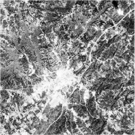
Figure 2: Band-1 of Sat-image2 (After histogram equalization).

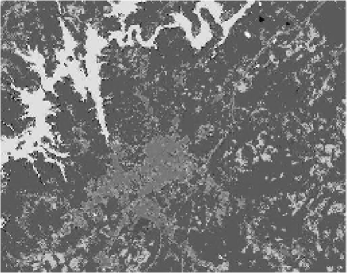
Figure 3: The ground truth for Sat-image2. The classes are represented by different colors.

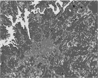
Figure 4: The classified image for Sat-image2. The classes are represented by different colors.

In Table 4 we include the results of four different random partitions of Sat-image2. It shows an excellent performance of the rule based classifiers. Both classifiers show consistent and comparable performances. For all partitions the softmin based classifiers show lower training errors while for the whole data the product based classifier performs better in only one case. Figure 2 shows one channel of Sat-image2 while Fig. 3 depicts the ground truth values where each class is represented by a distinct gray level. Fig. 4 shows a typical classification result (corresponding to the first partition) which is almost identical to Fig. 3.

The same data set (Sat-Image 2) has been used by Kumar et al. [25] in a comparative study using several classification techniques. The best result obtained by them using a fuzzy integral based scheme gives a classification rate 78.15%. In our case, even the worst performance is about 5% better than the results in [25].

In Table 5 we show the rules obtained for classes 1, 2 and 3 of Sat-image 2 using the training set 1. Column 1 of Table 5 shows the class number while column 2 lists the rule identification number. Column 3 describes the rules using the membership functions in the antecedent part of the rules. Since it is a seven dimensional data, each rule involves seven atomic antecedent clauses (fuzzy sets). Each fuzzy set is represented by a 2-tuple $(\mu_{i},\sigma_{i})$, where $\mu_{i}$ and $\sigma_{i}$ are the center and spread of a Gaussian membership function. Thus for rule number 2, the tuple (65.7,11.9) represents a clause ”gray value from channel 1 is CLOSE to 65.7” where the fuzzy set CLOSE to 65.7 is represented by a Gaussian function with center at 65.7 and spread 11.9. Inspection of the parameters of rules for class 1 reveals that between rule 2 and rule 6 all features change, but features 4, 5 and 7 changes significantly. Comparing rules 6 and 8 we find that features 3, 5, 6 and 7 change significantly. This indicates that each rule represents distinct areas in the feature space.

Table 5 also suggests that data from class 2 probably form a nice cluster in the feature space that can be modeled by just a single rule. This is further confirmed by the fact that the spread of the membership functions for features 2,4,5,6 and 7 are relatively small.

Similarly, for class 3, different rules model different areas in the feature space. For rules 14 and 15 although $\mu_{i}$’s for features 1 and 2 do not change much, the $\mu_{i}$’s for other features change considerably between the two rules. Depending on the complexity of the class structure, the required number of rules also changes. The number of rules for a given class may also vary depending on the training set used. However, this variation across the training sets is not much. For example, the number of rules for class 1 obtained using 4 training sets are 3, 2, 3 and 4 respectively. Similar results are obtained for other classes too. This indicates good robustness of the proposed rule generation and tuning algorithm.

4.2 Performance of the Classifiers with context sensitive inferencing

Table 6: Performance of the rule based classifiers designed with context-sensitive reasoning scheme for 4 different partitions of Sat-image1 data set.

Partition	Number of	% of Error
Number	Rules	Trng.	Test
1	27	11.0%	15.58%
2	26	9.8%	16.19%
3	25	12.8%	15.96%
4	19	9.6%	16.22%

Table 7: Classification performances designed with context-sensitive reasoning scheme for 4 different training sets for Sat-image2

Training	No. of	Error Rate in	Error Rate in
Set	rules	Training Data	Whole Image
1.	29	11.87%	13.5%
2.	24	14.6%	14.45%
3.	24	12.19%	13.18%
4.	25	12.75%	13.1%

To study the effect of context sensitive inferencing scheme on the classifiers we performed several experiments. First we tuned the set of rules obtained from the context tuning (context free inferencing) stage using softmin operators with fixed value of $q(=-10.0)$ parameters. In this experiment the values of $q_{i}$s for all the rules are initially set to -10.0, while the learning parameter $\eta_{q}=500$ and $maxiter=200$.

The performances of the context sensitive classifiers after conjunction operator tuning are summarized in Tables 6 and 7 for Sat-image1 and Sat-image 2 respectively. It can be observed that the performances in terms of classification rate do not improve significantly. However, some improvement in terms of training error as defined by (8) is observed in all cases. It is further seen that after tuning, the $q_{i}$s for all rules remain negative, which makes every rule to use approximately the minimum as the conjunction operator. This is hardly surprising, since the initial rules are already context tuned with fixed value of $q=-10.0$ for all rules. So it indicates that the context tuning with fixed $q$ has developed the rule set to correspond to an energy minima.

To investigate this issue further, we tuned the same initial set of rules (i.e., the context tuned rules with fixed $q=-10.0$) with different initial values of $q_{i}$s, namely, 1.0 and 5.0. All classifiers, with the same training data set has shown strong tendencies of convergence to similar set of conjunction operators, irrespective of the initial value of the $q_{i}$s. We present the result of the classifiers designed with the partition 1 of satimage-1 and satimage-2 with initial values of $q_{i}$s 1.0 and 5.0 in Table 8. The results for initial $q_{i}$ -10.0 are also included in this table for comparison. Column 2 of Table 8 (and 9) shows the initial value of q for all rules in the rule base when the q-tuning for every rule (to realize context sensitive inferencing) starts.

Table 8: Performance analysis of context sensitive inferencing for rule based classifiers (when the initial rules were context tuned with q=-10.0 for all rules)

Training	Initial	Training)		Training		Misclassification in test
data	$q_{i}$	Error ($E$)		Misclassification		data or whole image
		Initial	Final	Initial	Final	Initial	Final
Sat-image1	-10.0	176.26	175.9	54 (10.8%)	55 (11.0%)	925 (15.6%)	917 (15.4%)
	1.0	359.71	176.02	72 (14.4%)	55 (11.0%)	1000 (16.8%)	915 (15.4%)
	5.0	468.09	176.28	116 (23.2%)	54 (10.8%)	1536 (25.9%)	908 (15.3%)
Sat-image2	-10.0	688.07	685.06	192 (12.0%)	189 (11.8%)	35657 (13.6%)	35202 (13.4%)
	1.0	1283.42	724.98	274 (17.1%)	202 (12.6%)	37241 (14.2%)	35585 (13.5%)
	5.0	1487.01	684.86	414 (25.8%)	190 (11.8%)	50330 (19.2%)	35082 (13.4%)

Table 8 shows that for both cases with initial $q_{i}$s 1.0 and 5.0, though the initial value of error and misclassification rates are quite high, after the tuning they are much lower and very close to those corresponding to classifiers with initial $q_{i}$ -10.0 for the respective data set. This fact is reflected for the training sets as well as the test sets. It was further observed that for all the initial setting of $q_{i}$ the final values of $q_{i}$ become negative making the operator more or less equivalent to the $minimum$ operator. They are observed to attain values close in magnitude also. A small but interesting exception occurs in case of Satimage-2 (training set 1). Figure 5 shows the bar diagram of the tuned $q$ values of the rules for Satimage-2. In the figure each group of three bars shows the tuned $q$ values for a particular rule for three different initial values of $q=-10.0$ (white), 1.0 (gray) and 5.0 (black) respectively. For rule 1 with initial $q_{1}=1.0$, it can be observed that $q_{1}$ remains 1.0. We analyzed the case and found that the rule was not fired at all and the value remained the same as the initial value. The results in tables 8 and 9 suggest that the context tuning using softmin has successfully reduced the error and developed a set of rules such that the optimal performance of the classifiers can be obtained with minimum-like operators. Thus, it may be noted that for these two data sets direct use of minimum does an equally good job.

To investigate the validity of the above we carried out another set of experiments. Here we used the initial rule set as obtained from the prototype generation stage, i.e., the rules are no more context-tuned. We tuned these rules for initial $q_{i}$s -10.0, 1.0 and 5.0 respectively. The results of tuning for the partition 1 of Satimage1 and Satimage2 are summarized in Table 9. As evident from the results, in all the cases both initial and final performances are worse than those in the previous experiment. However, the results also reveal that the conjunction operator (context sensitive) tuning have produced substantial improvement of performances in all cases. Thus it shows that if the initial rule base is not very good, the context sensitive tuning can result in substantial improvement in performance.The bar plots of the tuned $q$ values of the rules for satimage-1 and satimage-2 are shown in figures 6 and 7 respectively. It can easily be discerned from the figures that the final set of $q_{i}$ values, unlike the previous experiment, differ substantially for different initial values of the $q_{i}$s. This clearly indicates that the system in this case attains different error minima in $q_{i}$-space for different initialization.

Table 9: Performance analysis of context sensitive inferencing for rule based classifiers (when the initial rules were not context tuned)

Training	Initial	Training)		Training		Misclassification in test
data	$q_{i}$	Error ($E$)		Misclassification		data or whole image
		Initial	Final	Initial	Final	Initial	Final
Sat-image1	-10.0	258.42	235.39	70 (14.0%)	67 (13.4%)	1035(17.4%)	958(16.14%)
	1.0	345.41	245.15	74 (14.8%)	67 (13.4%)	1097 (18.5%)	941 (15.8%)
	5.0	471.22	246.02	116 (23.2%)	68 (13.6%)	1680 (28.3%)	1042 (17.5%)
Sat-image2	-10.0	1198.47	1081.71	426 (26.6%)	398 (24.8%)	68070 (25.9%)	62873 (23.9%)
	1.0	1280.22	1096.01	417 (26.0%)	382 (23.8%)	63645 (24.2%)	56464 (21.5%)
	5.0	1446.36	1143.70	472 (29.5%)	404 (25.2%)	74299 (28.3%)	57174 (21.8%)

5 Conclusion

Fuzzy rule based classifiers are capable of dealing with data having different variances for different features and also different variances for different classes. In such a system a rule represents a region in the input space, which we call the context of the rule. Thus a fuzzy rule based classifier is inherently capable of detecting outliers also. Here we proposed a scheme for designing a fuzzy rule based classifier. It starts with generation of a set of prototypes. Then these prototypes are converted into fuzzy rules. The rules are then tuned with respect to their context. We have developed two variants of the context tuning algorithm, one for rules using product as conjunction operator and the other is used when the conjunction operator is softmin.

The rule based classifier is then used to classify multi-spectral satellite images and the performance obtained is excellent. The classifier performance may further be improved using features other than gray labels. Also use of other T-norms can alter the performance of the classifier. We are currently investigating all these possibilities.

If softmin is used as the conjunction operator, then using different values of the $q$ parameters of softmin for different rules, the rules can be made to use effectively different conjunction operators. Such a scheme is called context sensitive inferencing. We have developed an algorithm for tuning the $q$ parameters on per-rule basis.

Our experimental result suggests that if the context tuning (with fixed $q$ value for all rules) is carried out properly then subsequent context sensitive tuning offers marginal (if any) improvement. However, if the rules are not context tuned, the context sensitive inferencing can improve the performance of the classifier substantially.

Some other facts also came to light from these experiments. The results of $q$ tuning of the context-tuned rules suggest possible existence of a deep error minima with respect to the $q$ parameters to which the system reached for different initializations. But the results for the rule sets without context-tuning indicates that the system lands up in different minima for different initializations.

In light of above we can suggest two possible utility for using context sensitive reasoning for classification: (1) if the context tuning is not good enough, the performance may be enhanced with context sensitive reasoning and (2) the results of tuning the $q_{i}$s with different initializations may be used for judging the quality of a rulebase as a whole. This aspect is currently under further investigation.

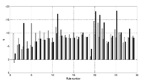
Figure 5: Bar diagram of $q_{i}$s of the rules for Sat-image2 for initial $q_{i}$ -10, 1 and 10 (when the initial rules were context tuned with q=-10.0 for all rules).

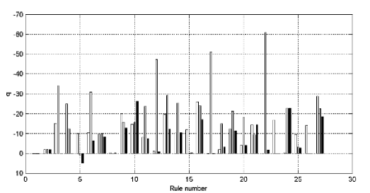
Figure 6: Bar diagram of $q_{i}$s of the rules for Sat-image1 for initial $q_{i}$ -10, 1 and 5 (when the initial rules were not context tuned).

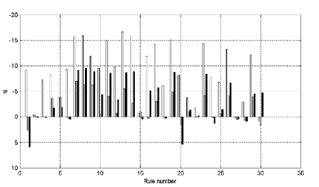
Figure 7: Bar diagram of $q_{i}$s of the rules for Sat-image2 for initial $q_{i}$ -10, 1 and 5 (when the initial rules were not context tuned).

References

- [1] R. O. Duda and P. E. Hart, Pattern Classification and Scene Analysis Wiley-Interscience, New York, 1974.
- [2] P. Gong, “Integrated Analysis of Spatial Data from Multiple Sources: Using Evidential Reasoning and Artificial Neural Network Techniques for Geological Mapping”, Photogrammetric Engineering and Remote Sensing, vol. 62, no. 5, pp. 513-523, 1996.
- [3] Gong, P. and D. J. Dunlop, Comments on Skidmore and Turner’s supervised nonparametric classifier, Photogrametric Engineering and Remote Sensing, 57(1):1311-1313, 1991.
- [4] J. C. Bezdek, Pattern Recognition with Fuzzy Objective Function Algorithms Plenum, New York, 1981.
- [5] J. C. Bezdek, J. Keller, R. Krishnapuram and N. R. Pal, Fuzzy Models and Algorithms for Pattern Recognition and Image Processing Kluwer, Massachusetts, 1999.
- [6] H. Ishibushi, T. Nakashima, T. Murata, “Performance Evaluation of Fuzzy Classifier Systems for Multi-Dimensional Pattern Classification Problems” IEEE Trans. on Syst. Man and Cybern: B, vol. 29, no. 5, pp. 601-618, 1999.
- [7] L. Kuncheva,Fuzzy Classifiers,Physica-Verlag,2000.
- [8] G. M. Foody, “Approaches for the production and evaluation of fuzzy land cover classifications from remotely-sensed data”, Int. J. of Remote Sensing, vol. 17, no. 7, pp. 1317-1340, 1996.
- [9] R. L. Cannon, J. V. Dave, J. C. Bezdek and M. M. Trivedi, “Segmentation of a thematic mapper image using the fuzzy c-means clustering algorithm”, IEEE Trans. Geosci. Remote Sensing, vol. GRS-24, no. 3, pp. 400-408, 1986.
- [10] A. Bárdossy and L. Samaniego, “Fuzzy rule-based classification of remotely sensed imagery”, IEEE Trans. Geosci. Remote Sensing, vol. 40, no.2 pp. 362-374, 2002.
- [11] T. Kohonen, “The self-organizing map,” Proc. IEEE, vol. 78, no. 9, pp. 1464-1480, 1990.
- [12] A. Laha and N. R. Pal “Dynamic generation of Prototypes with Self-Organizing Feature Maps for classifier design”, Pattern Recognition vol. 34, no. 2, pp. 315-321, 2000.
- [13] A. Laha and N. R. Pal “Some novel classifiers designed using prototypes extracted by a new scheme based on Self-Organizing Feature Map”,IEEE Trans. on Syst. Man and Cybern: B, vol 31, no. 6, pp. 881-890, 2001.
- [14] A. H. S. Solberg, A. K. Jain and T. Taxt, “Multisource classification of remotely sensed data: Fusion of Landsat TM and SAR images”, IEEE Trans. on Geosci. Remote Sensing, vol. 32, no. 4, pp. 768-777, 1994.
- [15] J. D. Paola and R. A. Schowengerdt, “A detailed comparison of backpropagation neural network and maximum likelihood classifiers for urban land use classification”, IEEE Trans. on Geosci. Remote Sensing, vol. 33, pp. 981-996, July, 1995.
- [16] T. Lee, J. A. Richards and P. H. Swain, “Probabilistic and evidential approaches for multispectral data analysis”,IEEE Trans. on Geosci. Remote Sensing, vol. GE-25, pp. 283-293, 1987.
- [17] J. A. Benediktsson, P. H. Swain and O. K. Ersoy, “Conjugate-gradient neural networks in classification of multisource and very high-dimension remote sensing data”, Int. J. Remote Sensing, vol. 14, pp. 2883-2903, 1993.
- [18] P. M. Atkinson and A. R. L. Tatnall, “Neural networks in remote sensing: An Introduction” Int. J. Remote Sensing, vol. 18, pp. 699-709, 1997.
- [19] H. Bischof, W. Schneider and A. J. Pinz, “Multispectral Classification of Landsat-Images Using Neural Networks”, IEEE Trans. on Geosci. Remote Sensing, vol. 30, no. 3, pp. 482-490, 1992.
- [20] J. J. Clark and A. L. Yuille, Data Fusion for Sensory Information Processing System, Kluwer Academic, 1990.
- [21] S. L. Chiu, “Fuzzy model identification based on cluster estimation,” J. Intell. and Fuzzy Syst., vol. 2, pp 267-278, 1994.
- [22] H. Dyckhoff and W. Pedrycz, “Generalized means as models of compensative connectives, Fuzzy Sets and Systems, vol. 14, pp. 143-154, 1984.
- [23] N. R. Pal and C. Bose, “ Context sensitive inferencing and “reinforcement type” tuning algorithms for fuzzy logic systems”, International Journal of Knowledge-Based Intelligent Engineering Systems, vol. 3, no. 4, pp. 230-239, 1999.
- [24] ftp://ftp.dice.ucl.ac.be/pub/neural-nets/ELENA
- [25] A. S. Kumar, S. Chowdhury and K. L. Majumder, “Combination of neural and statistical approaches for Classifying space-borne multispectral data,” Proc. of ICAPRDT99, pp. 87-91, 1999.