Analysis of a global Moreton wave observed on October 28, 2003

Abstract

We study the well pronounced Moreton wave that occurred in association with the X17.2 flare/CME event of October 28, 2003. This Moreton wave is striking for its global propagation and two separate wave centers, which implies that two waves were launched simultaneously. The mean velocity of the Moreton wave, tracked within different sectors of propagation direction, lies in the range of $v\approx 900-1100$ km s^-1 with two sectors showing wave deceleration. The perturbation profile analysis of the wave indicates amplitude growth followed by amplitude weakening and broadening of the perturbation profile, which is consistent with a disturbance first driven and then evolving into a freely propagating wave. The EIT wavefront is found to lie on the same kinematical curve as the Moreton wavefronts indicating that both are different signatures of the same physical process. Bipolar coronal dimmings are observed on the same opposite East-West edges of the active region as the Moreton wave ignition centers. The radio type II source, which is co-spatially located with the first wave front, indicates that the wave was launched from an extended source region ($\gtrsim 60$ Mm). These findings suggest that the Moreton wave is initiated by the CME expanding flanks.

1 Introduction

Large-scale, large-amplitude disturbances propagating in the solar atmosphere were first recorded by Moreton (1960) and Moreton & Ramsey (1960) in the chromospheric H${\alpha}$ spectral line; therefore called “Moreton waves”. Typical velocities are in the range $\approx 500-1000$ km s^-1, and the angular extents are $\approx 90-130\arcdeg$ (e.g. Warmuth et al., 2004a; Veronig et al., 2006). Since there is no chromospheric wave mode which can propagate at such high speeds, Moreton waves were interpreted as the intersection line of an expanding, coronal fast-mode shock wave and the chromosphere which is compressed and pushed downward by the increased pressure behind the coronal shockfront (Uchida, 1968). They occur in association with major flare/CME events and type II bursts (Smith & Harvey, 1971), the latter being a direct signature of coronal shock waves. Typically, the first wavefront appears at distances of $\geq$100 Mm from the source site and shows a circular curvature. The fronts are seen in emission in the center and in the blue wing of the H$\alpha$ spectral line, whereas in the red wing they appear in absorption. This behavior was interpreted as a downward motion of the chromospheric plasma with typical velocities of $\approx 5-10$ km s^-1 (Švestka, 1976). Sometimes the trailing segment of the wave shows the upward relaxation of the material, i.e., the chromosphere executes a down-up swing (Warmuth et al., 2004b). In the beginning of the wave propagation, the leading edge is rather sharp and intense. As the disturbance propagates, the perturbation becomes more irregular and diffuse and its profile broadens (Warmuth et al., 2001, 2004a). Thus, the perturbation amplitude decreases and the wavefronts get fainter until they can no longer be traced at $\approx 300-500$ Mm from the source active region (Smith & Harvey, 1971; Warmuth et al., 2004a).

A decade ago, large-scale waves were for the first time directly imaged in the corona by EIT (Extreme-Ultraviolet Imaging Telescope; Delaboudinière et al., 1995) aboard the SoHO (Solar and Heliospheric Observatory) spacecraft, so-called “EIT waves” (Thompson et al., 1997). Similarities in the propagation characteristics led to the assumption that in at least a fraction of the events are the EIT waves the coronal counterpart of the chromospheric Moreton waves (e.g. Thompson et al., 1997; Warmuth et al., 2001; Vršnak et al., 2002, 2006; Veronig et al., 2006). Basic questions regarding the nature of Moreton and EIT waves are whether they are caused by the same or by different disturbances, and whether they are initiated by the associated flare or the CME. For recent reviews, we refer to Chen et al. (2005), Mann & Klassen (2005), Warmuth (2007) and Vršnak & Cliver (2008).

Here, we study the fast and globally propagating Moreton wave that occurred in association with the powerful X17.2/4B flare and fast CME event from the NOAA AR10486 (S16$\arcdeg$, E08$\arcdeg$) on October 28, 2003. Due to its extreme powerfulness and geo-effectiveness, diverse aspects of this flare/CME event have been analyzed in a number of studies (e.g. Gopalswamy et al., 2005; Klassen et al., 2005; Aurass et al., 2006; Kiener et al., 2006; Hurford et al., 2006; Mandrini et al., 2007). The relationship of the Moreton wave to radio observations has already been studied in Pick et al. (2005). In this paper, we focus on the kinematical analysis of the Moreton wave, its relationship to the flare, the CME, coronal dimmings and type II radio bursts, in order to get insight into the wave characteristics and its initiating agent.

2 Data

We analyzed the Moreton wave of 2003 October 28 and associated phenomena (flare, EIT wave, coronal dimmings, type II radio burst) using the following data sets.

1. The Moreton wave is studied in H$\alpha$ filtergrams recorded by the Meudon Heliograph (France) which provides simultaneous observations of the full Sun at three different wavelengths in the H${\alpha}$ spectral lines (H${\alpha}$ line center, H${\alpha}$ $+$ 0.5 Å and H${\alpha}$ $-$ 0.5 Å) with an imaging cadence of $\sim$1 min.

2. The EIT wave and the coronal dimmings are studied in full-disk EUV images by EIT/SoHO (Delaboudinière et al., 1995). The analysis is conducted in the 195 Å bandpass which has a time cadence of $12$ min. The coronal dimmings are also analyzed with TRACE (Transition Region And Coronal Explorer, Handy et al., 1999). High-resolution 195 Å filtergrams with a field-of-view (FoV) of 380$\arcsec\times$340$\arcsec$ around the flare site are available with a time cadence of $\approx$ 8 sec.

3. The associated CME was observed by SoHO/LASCO (Brueckner et al., 1995). We use the information from the LASCO CME catalog at http://cdaw.gsfc.nasa.gov/cme_list/ (Yashiro et al., 2004).

4. The associated flare is studied in soft X-rays (SXRs) by the GOES10 satellite and in hard X-rays (HXRs) $>$150 keV provided by the spectrometer SPI onboard INTEGRAL (Kiener et al., 2006).

5. The associated type II radio burst is analyzed utilizing the dynamic radio spectrum recorded by the radio spectrographs of the Astrophysikalisches Institut Potsdam (AIP; Mann et al., 1992). Positions of the radio source are derived from observations of the Nançay Radioheliograph (NRH; Kerdraon & Delouis, 1997).

6. A full-disk magnetogram recorded by SoHO/MDI (at 11:00:03 UT; pixel size $\approx$ 2$\arcsec$) is used to study the magnetic context of the event (Scherrer et al., 1995).

3 Results

3.1 Event overview

The Moreton wave under study was launched during a powerful flare/CME event which occurred in NOAA AR10486 (S16$\arcdeg$, E08$\arcdeg$) on October 28, 2003. NOAA AR10486 had a complex magnetic configuration of $\beta\gamma\delta$ and was surrounded by several other large and complex ARs (e.g. AR10484, AR10488; see Fig. 1). The time range between 19-Oct-2003 and 4-Nov-2003 was characterized by an extremely high level of solar activity during which 12 X-class flares occurred. On 28-Oct-2003 AR10486 produced a X17.2/4B two-ribbon flare. The GOES10 SXR flux showed the flare onset in the 1$-$8 Å channel at $\approx$11:01 UT reaching peak at 11:10 UT. The INTEGRAL HXR observations cover the total flare impulsive phase which lasted roughly 15 min. The increase of the HXR flux ($>$150 keV) started at 11:02:00 UT and peaked for the first time at 11:02:40 UT. The associated fast halo CME had a mean plane of sky velocity $v\approx$ 2500 km s^-1 and its linear back-extrapolated launch time is 11:01 UT (LASCO CME catalogue, Yashiro et al. (2004)). This goes along with a filament activation in the southeastern quadrant at 11:01 UT.

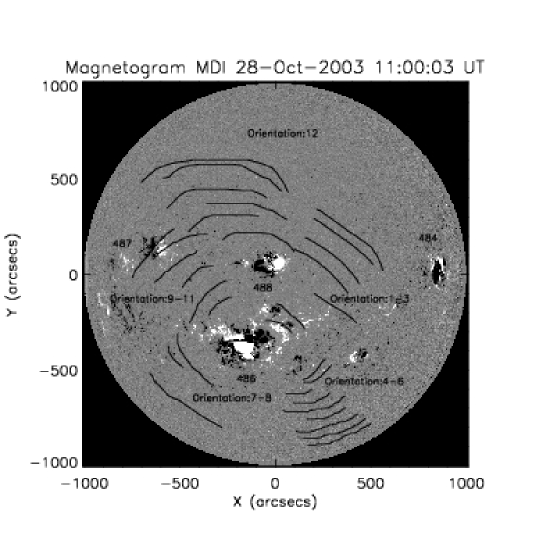
Figure 1: Leading edges of all wavefronts visible during the time interval 11:02 – 11:13 UT plotted on a MDI/SoHO magnetogram recorded at 11:00 UT. Active region (AR) numbers and the five sectors, in which the Moreton wavefronts were propagating, are indicated.

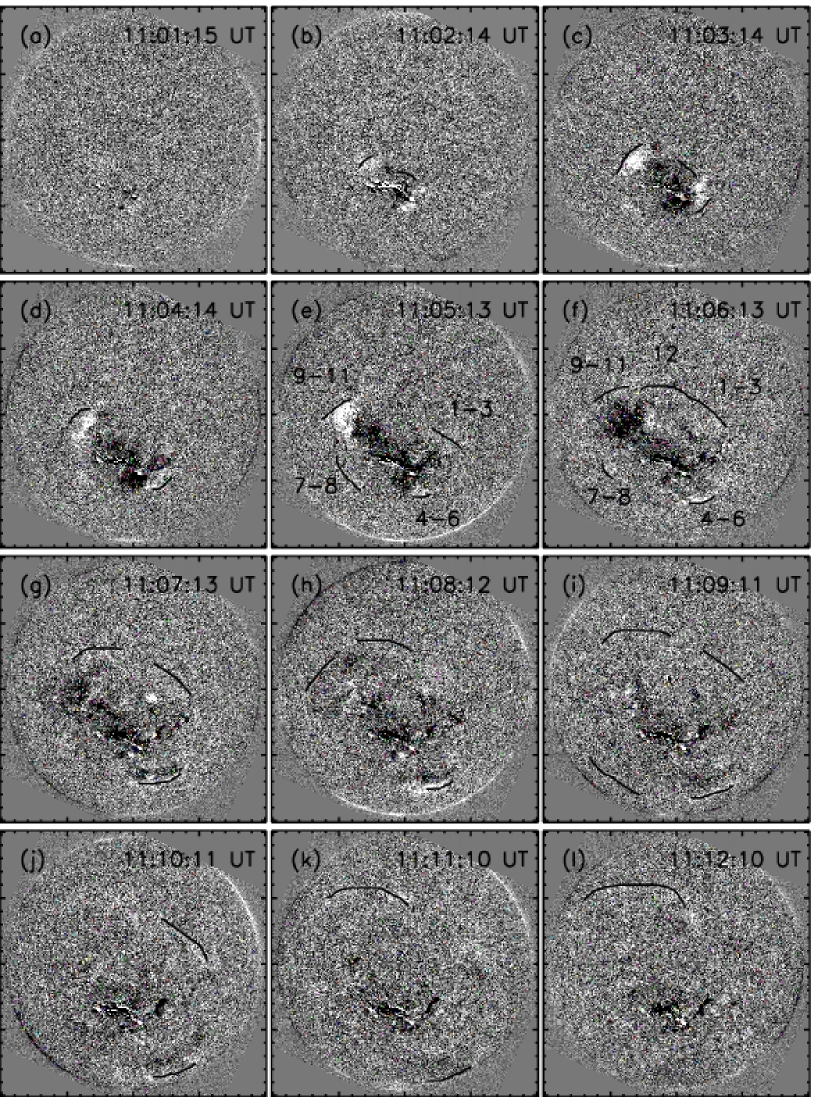
Figure 2: Sequence of H$\alpha$ blue-minus-red wing images after subtraction of a pre-event reference frame. The identified leading edges of the Moreton wavefronts (seen as bright fronts) are indicated by black lines for all different propagation directions. The corresponding sectors are indicated in images (e) and (f). Each image shows a FoV of 2000$\arcsec$ $\times$ 2000$\arcsec$ around Sun center.

The Moreton wave can be identified during the time interval 11:02–11:13 UT. The kinematics of the Moreton wave is analyzed applying two different methods. The first method relies on the visual determination of wavefronts in a series of difference images. The second one is based on the analysis of intensity profiles, derived along the wave fronts, so-called perturbation profiles.

3.2 Visual method

We subtracted red and blue wing filtergrams recorded simultaneously at H$\alpha+0.5\hbox{\AA}$ and H$\alpha-0.5\hbox{\AA}$ with the Meudon Heliograph. These images contain information on the plasma line-of-sight velocity (“dopplergrams”). In order to maximize the wave contrast, we produced difference images by further subtracting a blue-minus-red pre-event image (11:00 UT). Figure 2 shows this dopplergram sequence. The Moreton wave appears as a bright, arc-like transient disturbance, propagating away from the flare site in different directions, spanning almost over the complete solar disk. We studied the wave kinematics separately for four different directions, in which the wave could be distinctly followed. The four sectors 1$-$3, 4$-$6, 7$-$8, 9$-$11 (denoted by hours on the clock-face) and the visually identified wavefronts are indicated in Fig. 2. We note that the wavefronts in direction 9$-$11 were affected by refraction and reflection at the strong magnetic fields around AR 10488, which resulted in the wave propagation towards North after 11:06 UT (denoted as sector 12 in Fig. 2). The wave behavior in sector 12 is not considered in the following analysis.

The Moreton wave “radiant point” (source center) was estimated by applying circular fits to the earliest observed wavefronts for each propagation direction (see Fig. 3), whereby the projection effect due to the spherical solar surface was taken into account (following Warmuth et al., 2004a; Veronig et al., 2006). In order to estimate the error of the determined wave center, each of the earliest wavefronts was drawn for six times (first appearance) or four times (second appearance). The determined wave centers for the four directions are:
$[x,y]\approx[-253\arcsec\pm 31\arcsec,-307\arcsec\pm 6\arcsec]$ for direction 7–8,
$[x,y]\approx[-190\arcsec\pm 11\arcsec,-315\arcsec\pm 7\arcsec]$ for direction 9–11,
$[x,y]\approx[-51\arcsec\pm 16\arcsec,-376\arcsec\pm 8\arcsec]$ for direction 1–3, and
$[x,y]\approx[+69\arcsec\pm~{}9\arcsec,-381\arcsec\pm 14\arcsec]$ for direction 4–6.
The wave centers derived for the four propagation directions can be grouped into two significantly different radiant points at the mean coordinates $[x,y]\approx[-221\arcsec\pm 39\arcsec,-311\arcsec\pm 8\arcsec]$ and $[x,y]\approx[9\arcsec\pm 61\arcsec,-379\arcsec\pm 11\arcsec]$, on the East and West borders of the source AR (see Fig. 3). This suggests that the wave propagation to the East (7–8 and 9–11) and to the West (1–3 and 4–6) can be attributed to two different source sites. Accordingly, the wave kinematics are derived using two different source site coordinates.

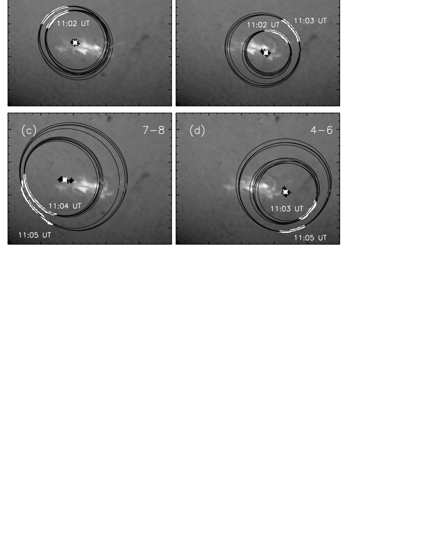
Figure 3: H${\alpha}$$-$0.5 Å image at 11:12 UT. The visually determined leading edges of the first and second visible wavefronts (marked as white lines) for the sectors (a) 9$-$11, (b) 1$-$3, (c) 7$-$8, (d) 4$-$6 are overlayed. The wavefronts were drawn several times in order to estimate errors (first wavefront: six times, second wavefront: four times). The superposed ellipses (black) correspond to fitted circles in the deprojected heliographic 2D plane, and are used for calculating the wave radiant points (black pluses) and their mean values (white crosses). The plotted FoV is $x$=[$-$600$\arcsec$, +400$\arcsec$], $y$=[$-$700$\arcsec$, +100$\arcsec$] with the origin at the solar disk center.

To derive the wave kinematics, we calculated for each point of the wavefronts its distance from the respective radiant point along great circles on the solar surface, and then averaged over all points of the wavefront. Figure 4 shows the distance-time diagrams for the four different propagation directions. The wave was first visible at a distance of $\approx$90 Mm from the wave’s radiant point in direction 1$-$3, and can be followed up to distances of 500–600 Mm in the different directions. In direction 4$-$6, the winking of a filament can be observed after the wave passage ($\approx$11:04 UT), which makes the wavefront determination difficult for this phase.

Linear and quadratic functions are fitted to the derived kinematical curves of the wave (see Fig. 4), from which we extrapolated the start times, ranging from 10:59:40 to 11:01:40 UT. The mean velocities derived from the linear fits are 940$\pm$10 km s^-1, 1050$\pm$10 km s^-1, 880$\pm$30 km s^-1, and 1020$\pm$20 km s^-1 for the orientations 1$-$3, 4$-$6, 7$-$8, and 9$-$11, respectively. The quadratic fits indicate wave deceleration for directions 1$-$3 and 9$-$11 with –1420$\pm$360 m s^-2 and –2960$\pm$280 m s^-2, respectively.

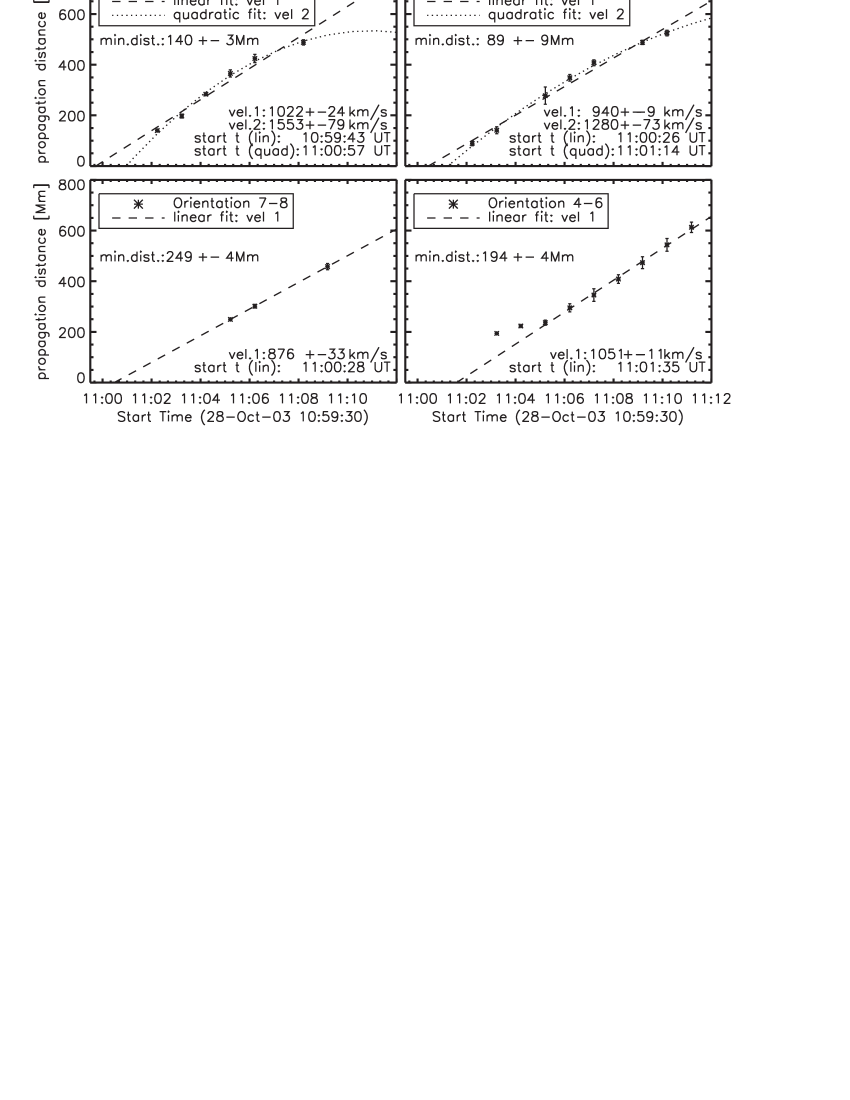
Figure 4: Kinematics of the Moreton wave. Distance vs. time diagrams derived separately for four different propagation directions (cf. Fig. 1). The dashed and dotted lines indicate the linear and quadratic fits to the kinematical curves, respectively. The first two data points for direction 4$-$6 were excluded in the fitting process, since they are uncertain due to the wave passage over a filament. Note that the error bars do not reflect uncertainties on the derived distances but deviations of the visually drawn wavefronts from the extrapolated circular shape in the deprojected heliographic 2D plane.

3.3 Perturbation profiles

In the second approach, the Moreton wave propagation was followed by analyzing the perturbation intensity-profiles $\Delta I(r,t)$. It has to be noted that the perturbation profile analysis can only be carried out if the disturbance is strong enough (see examples in Warmuth et al., 2004b). Moreton waves are in most cases too faint and irregular to be analyzed by this method. We also note that there are simplifying assumptions involved in the profile method: It is supposed that the ambient medium is homogeneous and the wavefronts expand circularly.

First of all, a specific sector is chosen for which the intensity evolution is calculated. Then the intensity values are averaged over annuli with a chosen angular width and a thickness of 5 Mm. This results in a mean intensity as a function of distance $r$ (measured along the solar chromosphere) from the wave’s radiant point. The procedure is repeated for each filtergram, until the Moreton wave fades away. Since we investigate intensity changes $\Delta I$, we use the blue-minus-red wing base-difference images, where the wave contrast is best.

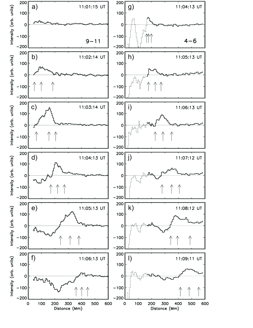
Figure 5: Perturbation profiles derived for the wave segments propagating in sectors 9–11 and 4–6. Arrows indicate the positions of the leading edge, the peak amplitude, and the trailing edge, respectively.

The method was carried out for the directions 9$-$11 and 4$-$6 because of their high intensities and their rather constant sector spans. However, the wavefronts become more and more irregular and show noticeable changes in their shape and propagation direction. Thus, with the profile method we can track the wave over shorter distances than with the visual method. The advantage of this method is that it provides us with more information on the perturbation characteristics. Figure 5 displays the perturbation profiles of the propagating wavefronts. From these profiles, the locations of the leading edge $r_{l}$, the trailing edge $r_{t}$ and the peak amplitude $r_{m}$ are extracted (see arrows in Fig. 5). The difference $\Delta r=r_{l}-r_{t}$ gives the width of the propagating disturbance.

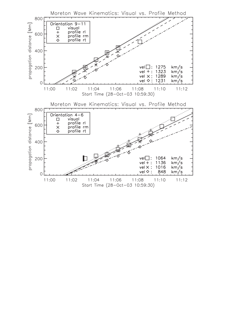
Figure 6: Kinematics of the Moreton wave (distance-time diagrams) derived from the perturbation profiles for orientation 9$-$11 and 4$-$6 (cf. Fig. 5). The pluses indicate the position of the leading edge $r_{l}$, the crosses the position of the peak amplitude $r_{m}$, and the diamonds the position of the trailing edge $r_{t}$. For comparison, we also plot the kinematics derived from the visual method (squares). The solid, dotted, dashed and dash-dotted lines indicate the linear fits to the data sets, respectively. The annotations vel $\Box$, vel $+$, vel $\times$ and vel $\diamond$ refer to the velocity values derived from the linear fits to the different time-distance data. The thick black vertical bar in direction 4–6 indicates the position of the type II burst within the measurement error (cf. Sect. 3.6).

From the calculated perturbation profiles, we derived the wave kinematics. Figure 6 shows the time-distance plots of the Moreton wave derived from the profile method, in comparison with the curves derived from the visual method. The extrapolated start times lie in the range of 11:00:40–11:01:50 UT, and correspond well to the starting times derived from the visual method. For the direction 9$-$11, the mean velocities derived from the linear fits are 1320 km s^-1, 1270 km s^-1 and 1230 km s^-1 for $r_{l}$, $r_{m}$ and $r_{t}$, respectively. The values for orientation 4$-$6 are 1140 km s^-1, 1040 km s^-1 and 850 km s^-1. The velocities derived by the profile method differ from those derived from the visual-method. However, this difference is not a result from the different methods, but merely results from the fact that with the profile method the late-phase evolution of the wave, when it has already decelerated, cannot be extracted. Using an identical time range for the fitting procedure for both methods (orientation 9–11: 11:02 UT – 11:06 UT; orientation 4–6: 11:04 UT – 11:09 UT), we obtain from the visual method mean velocities of 1280 km s^-1 and 1070 km s^-1, which is consistent with the velocities obtained from the profile method (peak amplitude) for the two sectors (cf. Fig. 6).

Figure 6 also indicates that the distance between the leading edge $r_{l}$, the peak amplitude $r_{m}$ and the trailing edge $r_{t}$ increases with time, which is especially prominent in direction 4–6. The peak amplitude of the perturbation increases in the beginning (see Fig. 5, panels g and h), and after achieving maximum (panel i), subsequently decreases (panels j to l). In direction 9–11, the wavefront steepens from panel a to c. We emphasize that panel c (11:03:14 UT) shows the situation close to the first appearance of the type II burst source (see Sect. 3.6), which reveals the formation of the coronal shock. The dip in the profile (at the trailing part of the wave) is a signature of the upward relaxation of the compressed chromospheric plasma. It is not visible in the beginning but becomes more and more remarkable as the wave evolves.

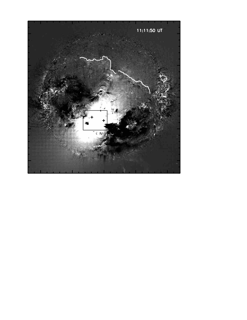
Figure 7: EIT base-difference image of 11:11:50 UT (reference image is 9:24:50 UT). The leading edge of the EIT wavefront is indicated by a white line. Coronal dimmings can be observed on both sides of the flare site (locally and globally). The black pluses show the two radiant points of the Moreton wave. The rectangle indicates the TRACE field of view (cf. Figure 9). The image shows a FoV of 2000$\arcsec$ $\times$ 2000$\arcsec$.

3.4 EIT wave

EIT images provide information on large-scale coronal changes associated with flare/CME events. Figure 7 shows a base-difference EIT 195 Å image at 11:11:50 UT (reference image is 9:24:50 UT). Due to the 12 min time cadence of the EIT instrument, the transient EIT wave (bright diffuse arcs toward North and Northwest of AR 10488) is observable in only one single frame at 11:11:50 UT in two sectors. It has already traveled across a significant portion of the solar disk. Since the EIT wave can only be traced in one single image, no kinematics can be derived. However, the position of the EIT wavefront can be compared to the Moreton wavefronts observed in H$\alpha$ (Fig. 8).

Figure 8 shows a combined plot of the Moreton wave kinematics (direction 1–3; visual method), the flare HXR flux measured by INTEGRAL, the back-extrapolated CME propagation curve (from the LASCO catalog) and the location of the EIT wavefront (direction 1–3). Extrapolating the 2nd order fit to the Moreton wave distance-time diagram in this direction, we find that the EIT wave is slightly ahead of the Moreton wave but basically on the same kinematical curve. The fact, that the EIT wavefront is located some 10 Mm ahead of the corresponding Moreton wave was also reported from other studies (e.g. Warmuth et al., 2004a; Veronig et al., 2006). Assuming that both are related phenomena, it can be explained by the different heights of the Moreton wave (chromosphere) and EIT wave (lower corona) observations and the inclination of the expanding coronal wave dome as envisaged in Uchida’s theory.

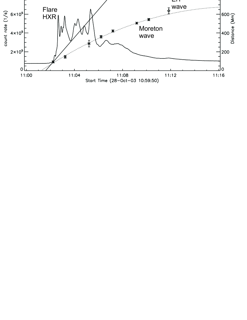
Figure 8: Kinematics of the Moreton wavefronts in direction 1$-$3 (visual method; displayed by asterisks) together with the second order fit, the position of the EIT wavefront at 11:12 UT in direction 1–3 (displayed by diamond), the linear back-extrapolated CME height-time curve, and the flare HXR flux above 150 keV.

3.5 Coronal Dimmings

Bipolar coronal dimmings are believed to be the footprints of large-scale flux-rope ejections (e.g. Hudson et al., 1997; Webb et al., 2000). In the event under study, coronal dimmings are detectable in EIT 195 Å (see Fig. 7) as well as TRACE 195 Å (see Fig. 9). EIT observations are available as full-disk images with a time cadence of $\approx$ 12 min. TRACE observations are available for a FoV of 380$\arcsec\times$340$\arcsec$ around the flare site with a high time cadence ($\approx$ 8 sec) during 10:14 UT and 11:45 UT. Figure 7 shows an EIT 195 Å base-difference image. It displays the global coronal dimmings, which are expanding over the whole hemisphere indicative of a complete restructuring of the corona (e.g. Zhukov & Veselovsky, 2007). In addition to these global or “secondary” dimmings (Mandrini et al., 2007), localized bipolar dimmings in the near vicinity of the flare site are also observed. These “core dimmings”, as quoted by Mandrini et al. (2007) are difficult to observe in EIT but are well captured with TRACE. Here, we focus on these small, bipolar dimming regions and their evolution.

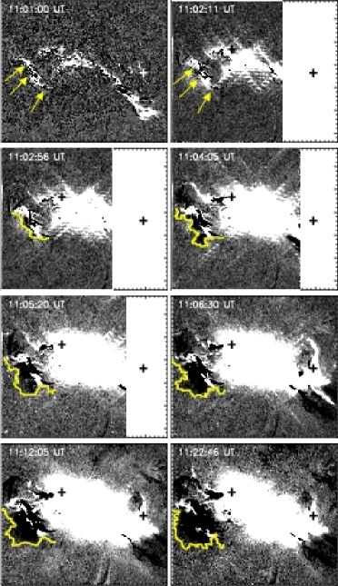
Figure 9: Evolution of the double coronal dimming region (black areas at East and West edges of the flare site). The pluses show the two derived radiant points of the Moreton wave. The plotted FoV is $380\arcsec\times 340\arcsec$ centered around [x,y]=$[-140\arcsec,-380\arcsec]$. The arrows and lines indicate the outer edge of the dimming region.

Figure 9 shows a sequence of TRACE 195 Å base-difference images. A pre-event image recorded at 10:59:26 UT was subtracted from the whole image series. At 11:00:29 UT we can observe the first small brightenings along the neutral line in AR10486. The first signature of the bipolar dimmings, which are observed as localized dark regions on each side of the flare site, can be detected at 11:01:00 UT (see Fig. 9). They lie on opposite east-west edges of the source AR and probably reflect the two CME expanding flanks. We also note that they are roughly located on the same axis as the two radiant centers of the wave. The time of first appearance of these bipolar dimming corresponds to the CME onset, which is determined from the linear back-extrapolation of the CME time-distance curve to be at $\approx$11:01 UT.

In the high cadence TRACE EUV images, we can study the evolution of the bipolar dimmings. Since the Western dimming region was only partially covered by the TRACE FoV (cf. Fig. 9), we concentrate here only on the Eastern dimming region. To obtain information on the area of the bipolar dimming regions, we used specific intensity levels and summed up the enclosed area (given in percentage of the entire solar disk; see Fig 10a).

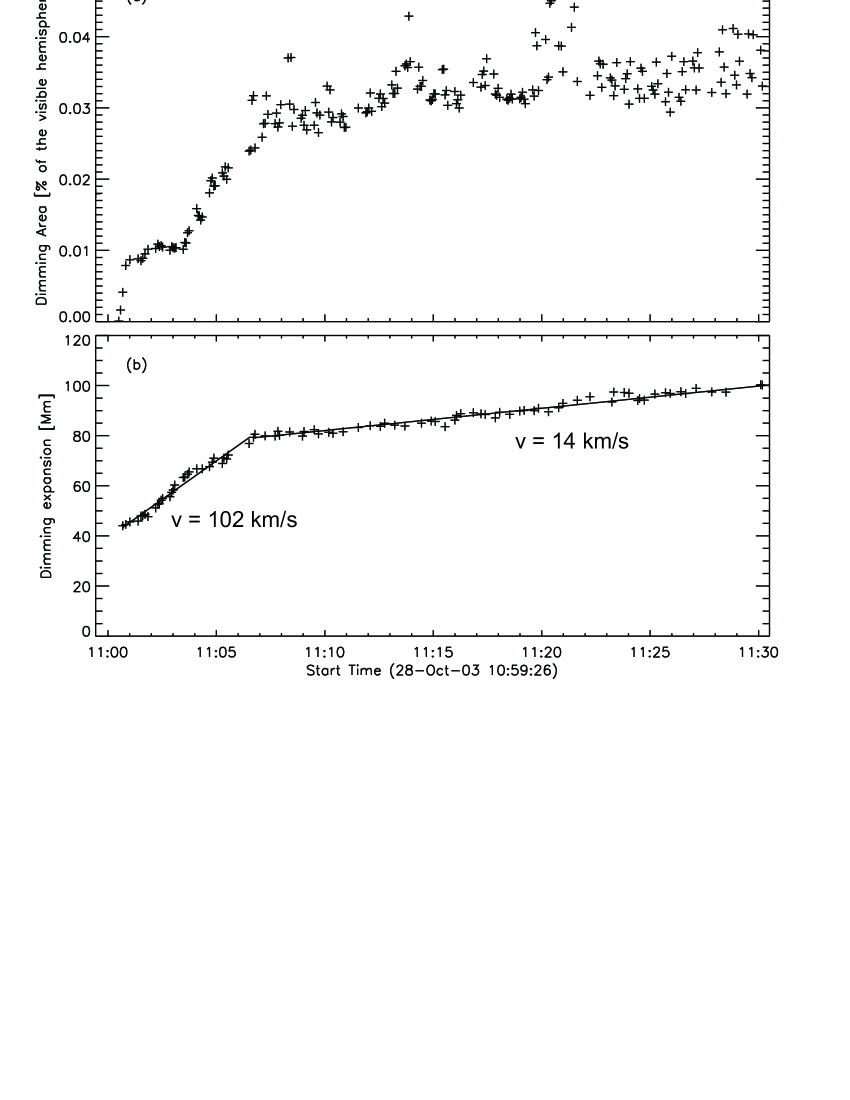
Figure 10: (a) Evolution of the area (in % of the visible solar hemisphere) occupied by the eastern coronal dimming region as measured from TRACE 195 Å images. (b) Kinematics of the outer border of the eastern coronal dimming region. Linear fits are applied separately to the early ($<$11:06 UT) and later evolution phase of the dimming.

The expansion velocity of the dimming regions (presumably related to the CME flanks) is derived by measuring the propagation of the outer edge of the dimming region, indicated by grey lines in Fig. 9. Figure 10b shows the distance-time diagram for the kinematics of the eastern dimming region. Due to the distinctive change in its propagation velocity, we applied two separate linear fits to the kinematical curve. The dimming shows a fast expansion ($v\approx 102$ km s^-1) until 11:06 UT, thereafter it drastically slows down by almost an order of magnitude to $v\approx 14$ km s^-1. We note that Fig. 10a and Fig. 10b show a similar evolution with fast growth up to $\approx$11:06 UT and much slower changes thereafter. At the time of the fast growth, the CME is in its initial phase.

3.6 Type II radio burst

According to Uchida (1968), Moreton waves appear at the intersection line of an expanding, coronal fast-mode shock and the chromosphere. Another shock signature are type II radio bursts (Uchida, 1974), excited by electrons accelerated at the shock front. Type II bursts usually show the fundamental and harmonic emission band, both frequently being split in two parallel lanes, so-called band-split (Nelson & Melrose, 1985). The interpretation of the band split as the plasma emission from the upstream and downstream shock regions, was affirmed by Vršnak et al. (2001). Thus the band-split can be used to obtain an estimate of the density jump at the shock front (Vršnak et al., 2002; Magdalenić et al., 2002). From that, one can infer the pressure jump, which governs the downward compression of the chromosphere after the shock-front passage.

We note that several aspects of the radio observations of this event were already analyzed by Klassen et al. (2005), Pick et al. (2005) and Aurass et al. (2006). The AIP dynamic radio spectrum (Fig. 11) shows complex and intense radio emission, consisting of a group of type III bursts, a type II bursts (Klassen et al., 2005), and a complex type IV burst. For a detailed dynamic spectrum covering frequency range 20 - 800 MHz, we refer to Fig. 4 in Pick et al. (2005).

In the present study we focus on the type II burst that started around 11:03 UT, at a frequency of 420 MHz. The back-extrapolation of the emission lanes point to 11:02:30 UT, i.e., close to the first peak of the HXR burst, and the intense type III bursts which indicate the impulsive phase of the flare. This is also close to the steepening phase of the Moreton wavefront of direction 9–11 (see Fig. 5, panel 3).

Nançay Radioheliograph measurements at 411 MHz at 11:03:01 UT and 11:03:11 UT show that the type II burst source was located at $\approx$ $(x,y)$=$(0.2~{}R_{\sun},-0.5~{}R_{\sun})$. Comparing the type II source location with the Moreton wave front, we find that the position of the radio source is cospatial with the first Moreton wave front in the direction 4$-$6. In Fig. 6 the position of the radio source is marked by a thick vertical bar, with the length of the bar corresponding to the measurement error.

The back-extrapolation of the type II burst to 11:02:30 UT indicates that the disturbance, which developed into a shock, was probably not launched before that time. On the other hand, we found the back-extrapolated start time of the Moreton wave to the western radiant point at 11:01:35 UT (see Fig. 4). This indicates that the Moreton wave was not launched from a point-like source but rather from an extended source. From Fig. 6 we find that at 11:02:30 UT the back-extrapolation of the Moreton wave trajectory was at a distance of $d\approx$ 60–80 Mm, which provides us with a lower limit for the source region size. The upper limit for the source region is given by the first appearance of the Moreton wave, which was at $\approx$ 200 Mm.

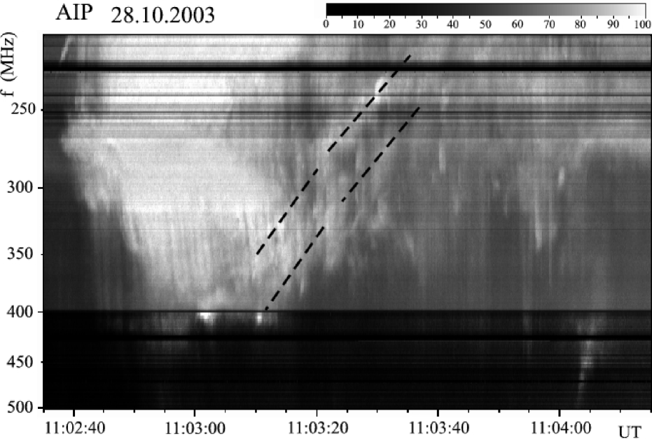
Figure 11: Dynamic radio spectrum recorded by AIP spectrographs, displaying the high-frequency part of the metric type II burst. The two dashed lines indicate the band split of the type II harmonic lane. The metric type II continues to decameter wavelengths.

Due to the complexity and overlapping of various radio emissions it is difficult to analyze in detail the high-frequency part of the type II burst. Nevertheless, in the period 11:03:10 to 11:03:40 UT, we were able to recognize a band-split pattern, with a relative bandwidth of $BDW=\Delta f/f\approx 0.15$ – 0.25 (see Fig. 11). The relative bandwidth $BDW$ is determined by the density jump at the shock front $X=\rho_{2c}/\rho_{1c}$, where $\rho_{1c}$ and $\rho_{2c}$ are the densities upstream and downstream of the shock front (for details see Vršnak et al., 2001). Since $BDW\equiv(f_{2}-f_{1})/f_{1}=\sqrt{\rho_{2c}/\rho_{1c}}-1$, we find $X_{c}=1.32$ – 1.56, where the subscript “c” stands for “corona”.

4 Interpretation and discussion

4.1 Source site and driver

We found two separate initiation centers for the Moreton wavefronts on opposite east-west edges of the source AR 10486. This implies that actually two waves were launched simultaneously. This argues against an initiation by the flare pressure pulse: first, a simultaneous launch of two flare pressure pulses is very unlikely; second, at the time of the first flare hard X-ray peak (11:02:40 UT), indicating the first episode of powerful flare energy release, we already observed the Moreton wave, this means that if initiated by the flare there would have been no time for the wave to reach a large amplitude to be observable. Nevertheless, we note that an initiation scenario caused by the flare cannot be completely excluded (for instance, assuming that the wave was launched already before the time of the first peak in the flare energy release).

The most likely interpretation of the observations is that the Moreton wave is caused by the expanding flanks of the CME, evidenced by the observed bipolar dimmings on east-west edges of the flare site. This is further strengthened by the observations of two Moreton wave radiant points, which lie roughly on the same axis as the bipolar dimmings. We also note that the initial acceleration of the wave coincides with the fast expanding phase of the dimming evolution with $v\approx$ 100 km s^-1, which lasts until 11:06 UT (cf. Fig. 10). This corresponds also well with the end of the steepening phase (presumably indicating the shock formation) of the Moreton wavefront profiles (cf. Fig. 5).

We also emphasize that the Moreton wave is not launched from two localized points but from two extended sources. This result is derived from the type II burst appearance revealing the shock formation, which is first detectable at $\approx$11:03 UT at a certain distance ($\approx$60 Mm) from the Moreton wave radiant point. At this time, the perturbation profiles of the Moreton wave are steepening (cf. Fig. 5). The surface of these extended source sites is located at a distance $d\approx 60-200$ Mm from the Moreton wave radiant points. The first value is determined from the type II occurrence, while the second value is given by the first Moreton wavefront appearance in this direction.

A strong relation between the CME lateral expansion and the occurrence of coronal shock waves was already suggested by radio observations. Pohjolainen et al. (2001) reported about a halo CME event, accompanied by a Moreton and an EIT wave, in which the appearance of new radio sources were attributed to the arc expansion of the CME magnetic field. Finally, the encounter of the propagating wave with magnetic field structures caused the opening of field lines. Maia et al. (1999) related the systematic occurrence of radio sources during the early evolution of a CME to the successive destabilization or interaction of loop systems which resulted in large-scale coronal restructering and finally CME formation. Similar conclusions are drawn by Temmer et al. (2009) comparing the Moreton wave observations of January, 17 2005 and the related type II burst resulting in an outcoming analytical MHD model.

4.2 Coronal shock characteristics

It can be presumed that at low heights the coronal shock is a quasi-perpendicular fast-mode MHD shock (Mann et al., 1999). Considering jump relations at the perpendicular shock front (e.g., Priest, 1982), the shock magnetosonic Mach number $M_{ms}=v_{c}/v_{ms}$ (where $v_{c}$ is the coronal shock velocity and $v_{ms}$ the magnetosonic speed) can be expressed as

$$M_{ms}=\sqrt{\frac{X_{c}(X_{c}+5+5\beta_{c})}{(4-X_{c})(2+5\beta_{c}/3)}}\,.$$ (1)

where $\beta_{c}$ is the ambient coronal plasma-to-magnetic pressure ratio and $X_{c}=\rho_{c2}/\rho_{c1}$ the density jump at the shock front. For the specific-heat ratio (the polytropic index) we have taken $\gamma=5/3$. Using $X_{c}=1.32$ – 1.56 for the density jump, as derived from the type II band-split observations (cf. Sect. 3.6), we find $M_{ms}=1.23$ – 1.42 for $\beta_{c}=1$, and $M_{ms}=1.25$ – 1.45 for $\beta_{c}=0.01$.

The pressure jump at the shock front, $P_{c}=p_{2c}/p_{1c}$, can be written as

$$P_{c}=~{}1+\frac{5M_{c}^{2}(X_{c}-1)}{3X_{c}}-\frac{X_{c}^{2}-1}{\beta_{c}}\,,$$ (2)

where $M_{c}$ represents the sound Mach number of the coronal shock, which for $\gamma=5/3$ reads:

$$M_{c}=~{}M_{ms}~{}\sqrt{1+\frac{6}{5\beta_{c}}}\,.$$ (3)

Using $X_{c}=1.32$ – 1.56, we find $P_{c}=2.82$ – 9.34 for $\beta_{c}=0.01$, and $P_{c}=1.61$ – 2.22 for $\beta_{c}=1$. Thus, the type II burst observations indicate that the pressure jump ranges between $\approx$ 2 and 10. The pressure jump at the shock front causes an abrupt pressure increase at the top of a given chromospheric element after the shock sweeps over it. Consequently, also a pressure discontinuity forms between the perturbed corona and the yet undisturbed chromosphere. The appearance of the pressure discontinuity at the top of the chromosphere implies that a downward-traveling shock should be formed. Behind the shock front the plasma is compressed and moves downwards (including the corona/chromosphere “interface”). As the shock penetrates deeper, a successively larger portion of the chromosphere is compressed and set into motion, increasing the H$\alpha$ blue-minus-red Doppler signal at the leading part of the Moreton wave.

Vourlidas et al. (2003) obtained from a CME case study that the speed and density of the CME front and flanks, derived from coronagraphic white light images, were consistent with the existence of a shock. Comparison of the observations with MHD simulations confirmed that the observed wave feature is a density enhancement from a fast-mode MHD shock (for further similar white light observations of coronal shocks see also Ontiveros & Vourlidas (2009)). Yan et al. (2006) found from radio imaging observations that the emitting sources of type III bursts were located at the compression region between the CME flanks and the neighboring open field lines. The compression region was revealed as a narrow feature in white light, and was interpreted as a coronal shock driven by the CME lateral expansion. It is occasionally also observed as a type IV-like burst propagating colaterally with the Moreton wave (Vršnak, 2005; Dauphin et al., 2006). Especially important are observations of broadening and intensity changes of UV emission lines in front of CMEs, associated with type II bursts, since such measurements provide an insight into the physical state of plasma in the compression region (Raymond et al., 2000; Mancuso et al., 2002; Ciaravella et al., 2005). Occasionally, the plasma parameters can be inferred also from the soft X-ray observations (Narukage et al., 2002).

5 Summary and Conclusions

We analyzed the intense Morton wave of October 28, 2003 together with its associated phenomena: the X17.2/4B flare event, the fast halo CME ($v\approx$ 2500 km s^-1), the EIT wave, the radio type II burst, and coronal dimmings, in order to study the wave characteristics and its driver. The main findings of the study and our interpretation are summarized in the following:

1. The Moreton wave propagates in almost all directions over the whole solar disk, and can be observed for a period as long as 11 min (during 11:02–11:13 UT). These are both unusual properties of a Moreton wave. But we note that a wave with similar characteristics (global propagation, $v\approx$ 1100$-$1200 km s^-1) was launched from the same AR on 2003 October 29 in assocation with an X10 flare/CME event (Balasubramaniam et al., 2007). We studied the wave kinematics in detail for four different propagation directions finding mean velocities in the range 900–1100 km s^-1. Typical values of the sound speed and the Alfv$\acute{\hbox{e}}$n speed in the solar corona are 180 km s^-1 and 300–500 km s^-1 (Mann et al. 1999), respectively, which corresponds to a magnetosonic Mach number of $\approx$2–3 of the Moreton wave under study, if interpreted as a propagating fast-mode shock. The band-split of the associated type II burst was determined to 0.15–0.25, from which we inferred magnetosonic Mach number $M_{s}=1.23-1.45$.

2. We find two radiant points (source centers) for the Moreton wave on opposite East-West edges of the source active region (AR 10486). This has not been reported before and indicates that either two independent waves were launched simultaneously, or that the wave was caused by the expansion of an extended source with a preferred axis.

3. The associated coronal wave (“EIT wave”) was observed by the EIT instrument in one frame. The determined EIT wavefront lies on the extrapolated kinematical curve of the Moreton wave, identifying both the EIT wave and the H$\alpha$ Moreton wave as different signatures of the same disturbance, according to Uchida’s theory.

4. In two propagation directions, a deceleration of $-2960$ m s^-2 and $-1420$ m s^-2 was observed in the distance-time diagrams of the H$\alpha$ Moreton wavefronts. In the initial phase, the perturbation profiles show amplitude growth and steepening of the disturbance. Later on, they display a broadening, amplitude decrease, and signatures of chromospheric relaxation appear at the trailing segment of the disturbance. This indicates that the coronal perturbation is a freely propagating large-amplitude simple-wave. The width of the disturbance is in the range of 50–150 Mm.

5. The extrapolated start time of the wave fits roughly with the extrapolated start time of the CME observed in LASCO (but we note that the uncertainty of the CME start time is of the order of 10 min) but occurs slightly before (2 min) the first HXR peak of the flare impulsive phase (cf. Fig. 8).

6. The associated bipolar coronal dimmings, which are generally interpreted as footprints of the expanding CME and associated coronal mass depletion, appear on the same opposite East-West edges of AR 10486 as the Moreton wave ignition centers do. The bipolar dimmings show a fast increase during the impulsive phase, followed by a much slower evolution, which indicates a characteristic restricted growth. The expansion velocity of the dimming region is $\approx$100 km s^-1 at the time, where the Moreton wave is launched.

7. The position of the type II burst source is co-spatial with the Moreton wavefront in direction 4$-$6. The back-extrapolated start time for the type II burst is $\approx$11:02:30 UT, i.e., somewhat later than the start time derived for the Moreton wave with respect to its radiant point. This suggests that the perturbation was not launched from a point-like source but from an extended source whose surface was at a distance $\gtrsim$60 Mm from the back-extrapolated radiant point. The launch time of the type II burst, which indicates the shock front formation, and the Moreton wave perturbation profile steepening coincide within the measurement errors.

From several case studies (e.g. Vourlidas et al., 2003; Mancuso et al., 2003; Yan et al., 2006; Cho et al., 2008; Ontiveros & Vourlidas, 2009) it was derived that radio as well as white light signatures in coronagraphs provide evidence that the lateral expansion of a CME is able to produce shocks in the corona. The results of the study, presented in this paper, support a scenario in which the launch of the observed Moreton and EIT wave is initiated by the lateral expansion of the CME. In such a case we expect that the perturbation is driven only over a short time/distance, as the CME lateral-expansion range is limited (for the theoretical background see, e.g. Žic et al., 2008; Temmer et al., 2009). Thus, the disturbance would evolve into a freely propagating wave, which is consistent with the observed perturbation characteristics. The behavior of CME expansion (radial and lateral direction) at low coronal heights might be an important condition for the formation of coronal shock waves.

References

- Aurass et al. (2006) Aurass, H., Mann, G., Rausche, G., & Warmuth, A. 2006, A&A, 457, 681
- Balasubramaniam et al. (2007) Balasubramaniam, K. S., Pevtsov, A. A., & Neidig, D. F. 2007, ApJ, 658, 1372
- Brueckner et al. (1995) Brueckner, G. E., Howard, R. A., Koomen, M. J., et al. 1995, Sol. Phys., 162, 357
- Chen et al. (2005) Chen, P. F., Fang, C., & Shibata, K. 2005, ApJ, 622, 1202
- Cho et al. (2008) Cho, K.-S., Bong, S.-C., Kim, Y.-H., et al. 2008, A&A, 491, 873
- Ciaravella et al. (2005) Ciaravella, A., Raymond, J. C., Kahler, S. W., Vourlidas, A., & Li, J. 2005, ApJ, 621, 1121
- Dauphin et al. (2006) Dauphin, C., Vilmer, N., & Krucker, S. 2006, A&A, 455, 339
- Delaboudinière et al. (1995) Delaboudinière, J.-P., Artzner, G. E., Brunaud, J., et al. 1995, Sol. Phys., 162, 291
- Gopalswamy et al. (2005) Gopalswamy, N., Yashiro, S., Liu, Y., et al. 2005, J. Geophys. Res. (Space Physics), 110, 9
- Handy et al. (1999) Handy, B. N., Acton, L. W., Kankelborg, C. C., et al. 1999, Sol. Phys., 187, 229
- Hudson et al. (1997) Hudson, H. S., Lemen, J. R., & Webb, D. F. 1997, in Astronomical Society of the Pacific Conference Series, Vol. 111, Magnetic Reconnection in the Solar Atmosphere, ed. R. D. Bentley & J. T. Mariska, 379
- Hurford et al. (2006) Hurford, G. J., Krucker, S., Lin, R. P., et al. 2006, ApJ, 644, L93
- Kerdraon & Delouis (1997) Kerdraon, A. & Delouis, J.-M. 1997, in Lecture Notes in Physics, Berlin Springer Verlag, Vol. 483, Coronal Physics from Radio and Space Observations, ed. G. Trottet, 192
- Kiener et al. (2006) Kiener, J., Gros, M., Tatischeff, V., & Weidenspointner, G. 2006, A&A, 445, 725
- Klassen et al. (2005) Klassen, A., Krucker, S., Kunow, H., et al. 2005, J. Geophys. Res. (Space Physics), 110, 9
- Magdalenić et al. (2002) Magdalenić, J., Vršnak, B., & Aurass, H. 2002, in ESA Special Publication, Vol. 506, Solar Variability: From Core to Outer Frontiers, ed. J. Kuijpers, 335–338
- Maia et al. (1999) Maia, D., Vourlidas, A., Pick, M., et al. 1999, J. Geophys. Res., 104, 12507
- Mancuso et al. (2002) Mancuso, S., Raymond, J. C., Kohl, J., et al. 2002, A&A, 383, 267
- Mancuso et al. (2003) Mancuso, S., Raymond, J. C., Kohl, J., et al. 2003, A&A, 400, 347
- Mandrini et al. (2007) Mandrini, C. H., Nakwacki, M. S., Attrill, G., et al. 2007, Sol. Phys., 244, 25
- Mann et al. (1992) Mann, G., Aurass, H., Voigt, W., & Paschke, J. 1992, in ESA Special Publication, Vol. 348, Coronal Streamers, Coronal Loops, and Coronal and Solar Wind Composition, ed. C. Mattok, 129–132
- Mann & Klassen (2005) Mann, G. & Klassen, A. 2005, A&A, 441, 319
- Mann et al. (1999) Mann, G., Klassen, A., Estel, C., & Thompson, B. J. 1999, in ESA Special Publication, Vol. 446, 8th SOHO Workshop: Plasma Dynamics and Diagnostics in the Solar Transition Region and Corona, ed. J.-C. Vial & B. Kaldeich-Schü, 477
- Moreton (1960) Moreton, G. E. 1960, AJ, 65, 494
- Moreton & Ramsey (1960) Moreton, G. E. & Ramsey, H. E. 1960, PASP, 72, 357
- Narukage et al. (2002) Narukage, N., Hudson, H. S., Morimoto, T., et al. 2002, ApJ, 572, L109
- Nelson & Melrose (1985) Nelson, G. J. & Melrose, D. B. 1985, Type II bursts (Solar Radiophysics: Studies of Emission from the Sun at Metre Wavelengths), 333–359
- Ontiveros & Vourlidas (2009) Ontiveros, V. & Vourlidas, A. 2009, ApJ, 693, 267
- Pick et al. (2005) Pick, M., Malherbe, J.-M., Kerdraon, A., & Maia, D. J. F. 2005, ApJ, 631, L97
- Pohjolainen et al. (2001) Pohjolainen, S., Maia, D., Pick, M., et al. 2001, ApJ, 556, 421
- Priest (1982) Priest, E. R. 1982, Solar magneto-hydrodynamics (Dordrecht, Boston: D. Reidel Pub. Co.), 74
- Raymond et al. (2000) Raymond, J. C., Thompson, B. J., St. Cyr, O. C., et al. 2000, Geophys. Res. Lett., 27, 1439
- Scherrer et al. (1995) Scherrer, P. H., Bogart, R. S., Bush, R. I., et al. 1995, Sol. Phys., 162, 129
- Smith & Harvey (1971) Smith, S. F. & Harvey, K. L. 1971, Physics of the Solar Corona, 27, 156
- Švestka (1976) Švestka, Z. 1976, Solar Flares (Dordrecht: Reidel)
- Temmer et al. (2009) Temmer, M., Vršnak, B., Žic, T., & Veronig, A. M. 2009, ApJ, 702, 1343
- Thompson et al. (1997) Thompson, B. J., Newmark, J. S., Gurman, J. B., St. Cyr, O. C., & Stezelberger, S. 1997, in Bulletin of the American Astronomical Society, Vol. 29, Bulletin of the American Astronomical Society, 884
- Uchida (1968) Uchida, Y. 1968, Sol. Phys., 4, 30
- Uchida (1974) Uchida, Y. 1974, Sol. Phys., 39, 431
- Veronig et al. (2006) Veronig, A. M., Temmer, M., Vršnak, B., & Thalmann, J. K. 2006, ApJ, 647, 1466
- Vourlidas et al. (2003) Vourlidas, A., Wu, S. T., Wang, A. H., Subramanian, P., & Howard, R. A. 2003, ApJ, 598, 1392
- Vršnak (2005) Vršnak, B. 2005, EOS Transactions, 86, 112
- Vršnak et al. (2001) Vršnak, B., Aurass, H., Magdalenić, J., & Gopalswamy, N. 2001, A&A, 377, 321
- Vršnak & Cliver (2008) Vršnak, B. & Cliver, E. 2008, Sol. Phys., in press
- Vršnak et al. (2002) Vršnak, B., Warmuth, A., Brajša, R., & Hanslmeier, A. 2002, A&A, 394, 299
- Vršnak et al. (2006) Vršnak, B., Warmuth, A., Temmer, M., et al. 2006, A&A, 448, 739
- Warmuth (2007) Warmuth, A. 2007, in Lecture Notes in Physics, Berlin Springer Verlag, Vol. 725, Lecture Notes in Physics, Berlin Springer Verlag, ed. K.-L. Klein & A. L. MacKinnon, 107
- Warmuth et al. (2001) Warmuth, A., Vršnak, B., Aurass, H., & Hanslmeier, A. 2001, ApJ, 560, L105
- Warmuth et al. (2004a) Warmuth, A., Vršnak, B., Magdalenić, J., Hanslmeier, A., & Otruba, W. 2004a, A&A, 418, 1101
- Warmuth et al. (2004b) Warmuth, A., Vršnak, B., Magdalenić, J., Hanslmeier, A., & Otruba, W. 2004b, A&A, 418, 1117
- Webb et al. (2000) Webb, D. F., Cliver, E. W., Crooker, N. U., Cry, O. C. S., & Thompson, B. J. 2000, J. Geophys. Res., 105, 7491
- Yan et al. (2006) Yan, Y., Pick, M., Wang, M., Krucker, S., & Vourlidas, A. 2006, Sol. Phys., 239, 277
- Yashiro et al. (2004) Yashiro, S., Gopalswamy, N., Michalek, G., et al. 2004, J. Geophys. Res. (Space Physics), 109, 7105
- Zhukov & Veselovsky (2007) Zhukov, A. N. & Veselovsky, I. S. 2007, ApJ, 664, L131
- Žic et al. (2008) Žic, T., Vršnak, B., Temmer, M., & Jacobs, C. 2008, Sol. Phys., 253, 237