NLO Polarized Chargino pair Production in Electron Positron Annihilation

Abstract

We calculate the complete one-loop quantum corrections to the helicity eigenstate chargino pair production cross sections in polarized electron positron collisions, within the Minimal Supersymmetric Standard Model. We calculate the non-QED corrections using the helicity amplitudes formalism, and Dimensional Regularization to deal with ultraviolet divergences. We calculate QED corrections using the dipole subtraction formalism to extract soft and collinear divergences in Bremsstrahlung, canceling them with the infrared divergences from virtual QED corrections. We show numerical results for the Focus Point scenario in mSUGRA, where we find important quantum corrections for differential cross sections with definite chargino helicities.

I Introduction

In supersymmetry the fermionic partners of charged Higgs and $W$ gauge bosons, the higgsinos and winos, mix to form a pair of charged fermions called charginos, $\tilde{\chi}_{i}^{\pm}$ Haber:1984rc . In many supersymmetric scenarios they are light enough to be produced at the LHC and ILC, although they have not yet been observed Abbiendi:2003sc ; Abdallah:2003xe ; Heister:2002mn ; Acciarri:1999km ; Aaltonen:2008pv ; Abazov:2009zi . The discovery of heavy charged fermions Polesello:2004aq ; Blumenschein:2005ms not coupled through strong interactions is not proof of supersymmetry, though. Precise measurements of their masses and couplings Kalinowski:1998yn should exhibit the supersymmetric prediction that SM couplings have their mirror coupling with superpartners. For example, $WWZ$ coupling should be equal to the $Z$ coupling to a pair of winos. This, together with the experimental precision expected at the ILC, leads to the necessity to have precise theoretical calculations for the observables in order to properly compare them with the experimental results.

Quantum corrections to chargino masses Pierce:1993gj ; Eberl:2001eu ; Fritzsche:2002bi ; Schofbeck:2007ib , chargino production cross section in electron positron collisions Diaz:1997kv ; Ellis:1998jk ; Oller:2005xg ; Kilian:2006cj ; Robens:2006np ; Blank:2000uc ; Kiyoura:1998yt , chargino production cross section in hadron colliders Hao:2006df , and chargino decays Fujimoto:2007bn ; Zhang:2001rd , are well documented. Here we improve the collective knowledge by presenting a complete one-loop calculation to the production cross section of polarized charginos in collisions between polarized electrons and positrons Diaz:2001vm ; Diaz:2000hi ; Diaz:2002rr ; Baer:2002bb . We stress the fact that this is the first time complete NLO corrections to the production of polarized charginos are calculated. These quantum corrections are an effect of the rich electroweak properties of the MSSM, and may provide a window to the Parity violating structure of this supersymmetric model. The full potential of this calculation will become available when quantum corrections to polarized chargino decays are incorporated, as indicated by the tree-level analysis of the importance of spin correlation between chargino production and decay gudrid .

In order to handle the full one-loop calculation we use form-factors to organize the bubble and triangular diagrams, and $Q$-charges to merge form-factors with box diagrams. We use the helicity amplitude formalism Diaz:2001vm ; Diaz:2000hi ; Diaz:2002rr to keep track of the electron and positron polarizations and the chargino helicities. To calculate the QED corrections and cancel the Infrared (IR) divergences we use the dipole subtraction formalism introduced in Dittmaier:1999mb . In this method the IR divergences are isolated analytically through the introduction of auxiliary subtraction functions. In this way, an IR cutoff is not needed, avoiding unpleasant numerical problems that emerge when a cutoff is used to regularize the infinities. At the end, the three body phase space integral is performed using a Monte Carlo method.

II Chargino Production at Tree Level

In the MSSM, the scattering $e^{+}e^{-}\to\tilde{\chi}^{+}\tilde{\chi}^{-}$ arises at tree level through $\gamma$ and $Z$ in the s-channel, and through $\tilde{\nu}_{e}$ in the t-channel, as indicated in Fig. 1.

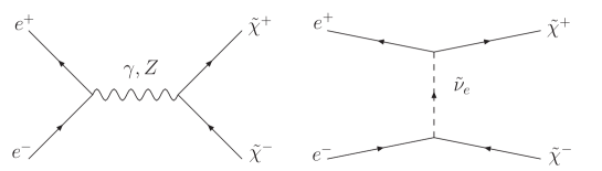
Figure 1: Three level diagrams for chargino pair productions at the ILC.

In this article we include the effects of the polarization of the electron and positron, and the chargino helicities. The notation for the four-momenta is as follows,

$$e^{+}(p_{2})+e^{-}(p_{1})\rightarrow\tilde{\chi}^{+}_{b}(k_{2})+\tilde{\chi}^{-}_{a}(k_{1})$$ (1)

where the convention is that $p_{1}$ and $p_{2}$ are incoming and $k_{1}$ and $k_{2}$ are outgoing four-momenta. The $Z$-coupling to two electrons is,

$${\cal G}_{Zee}^{\mu,0}=-{g\over{2c_{W}}}\gamma^{\mu}\left[g^{e}_{V}-g^{e}_{A}\gamma_{5}\right]$$ (2)

where $c_{W}=\cos\theta_{W}$, $s_{W}=\sin\theta_{W}$, and $\theta_{W}$ the weak mixing angle, with $\sin^{2}\theta_{W}^{\overline{MS}}(m_{Z})=0.23122$ Yao:2006px . Also $g^{e}_{V}=-1/2+2s_{W}^{2}$ and $g^{e}_{A}=-1/2$ are the vector-axial couplings. The $SU(2)$ gauge coupling constant $g$ is related to the positron electric charge by $g=s_{W}e$, with $\alpha(m_{Z})=e^{2}/4\pi=1/127$ AguilarSaavedra:2005pw . We also work with $m_{Z}=91.1876\pm 0.0021$ GeV and $\Gamma_{Z}=2.4952\pm 0.0023$ GeV Abbiendi:2000hu for the mass and width of the $Z$ boson respectively. The $Z$-coupling to a pair of charginos is,

$${\cal G}_{Z\chi\chi}^{ab\,\nu,0}={g\over{c_{W}}}\gamma^{\nu}\Big{[}O^{\prime L}_{ab}\frac{1-\gamma_{5}}{2}+O^{\prime R}_{ab}\frac{1+\gamma_{5}}{2}\Big{]}$$ (3)

where we use the notation in ref. Haber:1984rc for the $O^{\prime}_{L}$ and $O^{\prime}_{R}$ couplings.

The photon couplings to a pair of electrons and a pair of charginos is simply given by their electric charge,

$${\cal G}_{\gamma ee}^{\mu,0}=e\gamma^{\mu}\,,\qquad{\cal G}_{\gamma\chi\chi}^{ab\,\nu,0}=-e\gamma^{\nu}\delta_{ab}$$ (4)

Note that our convention is that a positive chargino is the particle and a negative chargino is the anti-particle.

The couplings between electrons charginos and sneutrinos are,

$${\cal G}_{\tilde{\nu}_{e}e\chi}^{b+,0}=-gV_{b1}\frac{1+\gamma_{5}}{2}C\,,\qquad{\cal G}_{\tilde{\nu}_{e}e\chi}^{a-,0}=C^{-1}gV_{a1}\frac{1-\gamma_{5}}{2}$$ (5)

where the matrix $V$ is one of the matrices that diagonalize the chargino mass matrix, in the notation of Haber:1984rc , and we are assuming CP is conserved and couplings are real. The matrix $C$ is the charge conjugation matrix, and appears due to the clashing arrows in the sneutrino Feynman diagram in Fig. 1. Only experimental lower bounds for the sneutrino mass have been set, of which we mention $m_{\tilde{\nu}_{e}}>94$ GeV Abdallah:2003xe .

III Quantum Corrections

We regularize divergent diagrams using dimensional reduction $\overline{DR}$. In each graph, divergences are contained in the parameter

$$\Delta={2\over{4-n}}+\ln 4\pi-\gamma_{E}$$ (6)

where $\gamma_{E}$ is the Euler-Mascheroni constant, and $n$ is the number of space-time dimensions, which is defined to be $n=4-2\epsilon$, with the limit $\epsilon\rightarrow 0$ to be taken at the end of the calculation. We call the renormalization subtraction point $Q$, and it is such that the parameters that define the tree-level cross section are promoted to $\overline{DR}$ running parameters, evaluated at the scale $Q$. We perform our calculations from first principles, not relying on loop calculating packages, as a way to find an independent result from groups that use these packages.

We have two types of divergences. The ultra-violet (UV) divergences appear at large internal momenta running in the loops, and they are to be cancelled with counterterms introduced by the renormalization procedure. We also have diagrams with infrared (IR) divergences, which appear at low internal momenta. These IR divergences are cancelled by bremsstrahlung, i.e., real photon emissions when the photon is soft or collinear.

We organize the calculation combining two formalisms, the form-factors and the helicity $Q$-charges. The form-factor formalism is specially useful to organize bubbles and triangle graphs, introduced in ref. Diaz:1997kv in the context of the quark-squark approximation, in which only quark and squark loop corrections are taken into account. The helicity amplitude formalism is necessary when boxes are included, and was introduced in ref. Diaz:2001vm where non-QED boxes were considered. It is specially designed to keep track of the polarization of the electrons and positrons and the helicity of the charginos, in the context of full one-loop calculation we are dealing with in this paper. We describe and combine both formalisms below.

III.1 Form-Factor Formalism

In ref. Diaz:1997kv we calculated the radiative corrections to chargino production in electron-positron collisions in the approximation where only loops from quark and squarks were considered. A form-factor formalism was developed, and here we generalize it to include triangular graphs in the gauge boson vertices to electron-positron pairs as well.

We organize the triangle graphs with the help of form-factors that define Green’s functions where the fermionic lines are on-shell, but the bosonic line are not. In the case of $Z$ couplings to a pair of charginos, they are given by

$${\cal G}_{Z\chi\chi}^{ab\,\mu}=F_{Z\chi\chi}^{vR}\,\gamma^{\mu}\frac{(1+\gamma^{5})}{2}\,+\,F_{Z\chi\chi}^{vL}\,\gamma^{\mu}\frac{(1-\gamma^{5})}{2}\,+\,F_{Z\chi\chi}^{sR}\,\frac{k_{-}^{\mu}}{\sqrt{s}}\frac{(1+\gamma^{5})}{2}\,+\,F_{Z\chi\chi}^{sL}\,\frac{k_{-}^{\mu}}{\sqrt{s}}\frac{(1-\gamma^{5})}{2}$$ (7)

and similarly for ${\cal G}_{\gamma\chi\chi}^{ab\,\mu}$ replacing $Z\rightarrow\gamma$ in the form-factors. The $v$ and $s$ labels refer to vector and scalar couplings respectively. We define $k_{-}=k_{1}-k_{2}$, which is normalized by $\sqrt{s}$ in order to make the form-factors dimensionless. Note that in ref. Diaz:1997kv we used a slightly different but easily related definition for the form-factors.

In the case of $e^{\pm}$–sneutrino–chargino vertices the form-factors are,

$${\cal G}_{\tilde{\nu}e\chi}^{b+}=F_{\tilde{\nu}e\chi}^{+}\frac{(1+\gamma^{5})}{2}C\,,\qquad{\cal G}_{\tilde{\nu}e\chi}^{a-}=F_{\tilde{\nu}e\chi}^{-}C^{-1}\frac{(1-\gamma^{5})}{2}$$ (8)

where $C$ is the charged conjugation matrix. In eq. (8), the $\pm$ notation refers to the positive (negative) outgoing chargino.

Here we extend the formalism in ref. Diaz:1997kv to include form-factors in the electron-positron vertex to a gauge boson,

$${\cal G}_{Zee}^{\mu}=F_{Zee}^{vR}\,\gamma^{\mu}\frac{(1+\gamma^{5})}{2}\,+\,F_{Zee}^{vL}\,\gamma^{\mu}\frac{(1-\gamma^{5})}{2}$$ (9)

and similarly for the photon. Only vector form-factors are needed because scalar ones disappear when electrons and positrons are taken on-shell. Also note that in the quark-squark approximation used in ref. Diaz:1997kv none of the $Zee$ form-factors receive quantum corrections.

We list below the form-factors that do not vanish at tree-level,

$$F_{Z\chi\chi}^{vR,0} {\hskip-46.94687pt}=\frac{g}{c_{W}}O^{\prime R}_{ab}\,,\qquad F_{Z\chi\chi}^{vL,0}=\frac{g}{c_{W}}O^{\prime L}_{ab}$$

$$F_{\gamma\chi\chi}^{vR,0} {\hskip-51.21504pt}=-e\delta_{ab}\,,\qquad F_{\gamma\chi\chi}^{vL,0}=-e\delta_{ab}$$

$$F_{\tilde{\nu}e\chi}^{+,0} {\hskip-49.79231pt}=-gV_{b1}\,,\qquad F_{\tilde{\nu}e\chi}^{-,0}=gV_{a1}$$ (10)

$$F_{Zee}^{vR,0} =-\frac{g}{2c_{W}}(g^{e}_{V}-g^{e}_{A})\,,\qquad F_{Zee}^{vL,0}=-\frac{g}{2c_{W}}(g^{e}_{V}+g^{e}_{A})$$

$$F_{\gamma ee}^{vR,0} {\hskip-73.97733pt}=e\,,\qquad F_{\gamma ee}^{vL,0}=e$$

We highlight a few details about these tree-level form-factors. First, the difference in sign between $F_{\gamma\chi\chi}$ and $F_{\gamma ee}$ is due to the fact we consider electrons and positive charginos as particles, and positrons and negative charginos as anti-particles, and of course $F_{\gamma\chi\chi}$ is proportional to $\delta_{ab}$ due to electromagnetic gauge invariance. Also, we note that the form-factors $F_{\tilde{\nu}e\chi}$ indicate that the wino component of the chargino is the one that couples to the sneutrino, diminishing considerably the $t$-channel contribution in the case of higgsino like charginos. In contrast, since,

$$O^{\prime R}_{ab}=-U_{a1}U_{b1}-\textstyle{\frac{1}{2}}U_{a2}U_{b2}+s_{W}^{2}\delta_{ab}\,,\qquad O^{\prime L}_{ab}=-V_{a1}V_{b1}-\textstyle{\frac{1}{2}}V_{a2}V_{b2}+s_{W}^{2}\delta_{ab}\,,$$ (11)

we see that both the wino and higgsino components of the charginos couple to the $Z$ gauge boson. Finally, we note that since $\sin^{2}\theta_{W}$ is approximately equal to $1/4$, the $Z$ vector coupling $g^{e}_{V}$ to a pair of electrons is much smaller that the axial one $g^{e}_{A}$. As a consequence, $F_{Zee}^{vR,0}$ $F_{Zee}^{vL,0}$ are nearly equal in magnitude but with opposite sign, which in turn implies a cancellation in the right handed electron cross sections. This cancellation will become more clear in the following section.

III.2 Helicity Amplitudes Formalism

The helicity amplitude formalism is a very systematic and economic way to organize virtual corrections through the so called $Q$-charges, introduced in Diaz:2001vm . Here we calculate also QED corrections not included in the above reference.

Consider the scattering amplitude for electron-positron into a pair of charginos. On the one hand, the electron has a polarization $\alpha=R,L$ and momentum $p_{1}$, while the positron has opposite polarization and momentum $p_{2}$. On the other hand, the negatively charged anti-chargino has a mass $m_{\chi_{a}}$, momentum $k_{1}$, and helicity $\lambda_{1}$, while the positively charged chargino has a mass $m_{\chi_{b}}$, a momentum $k_{2}$, and helicity $\lambda_{2}$. The dimensionless scattering amplitudes are written as,

$${\cal A}^{\alpha}_{\lambda_{2},\lambda_{1}}\ =\ \frac{1}{s}L_{\mu\alpha}\,Q_{\alpha i}^{\mu}\,\langle k_{2},\lambda_{2}|\Gamma^{i}|k_{1},\lambda_{1}\rangle.$$ (12)

where there is no sum on $\alpha$. The normalization is such that the differential scattering cross section is

$$\frac{d\sigma(\alpha,\lambda_{2},\lambda_{1})}{d\cos\theta}\ =\ \frac{\lambda^{1/2}(1,m_{\chi_{a}}^{2}/s,m_{\chi_{b}}^{2}/s)}{32\,\pi\,s}\left|{\cal A}^{\alpha}_{\lambda_{2},\lambda_{1}}\right|^{2},$$ (13)

and $\lambda(x,y,z)\equiv x^{2}+y^{2}+z^{2}-2xy-2xz-2yz$. The leptonic matrix elements are,

$$L_{\mu\alpha}=\bar{v}(p_{2})\gamma_{\mu}\frac{(1\pm\gamma^{5})}{2}u(p_{1})$$ (14)

with the $+(-)$ sign for $\alpha=R(L)$. Note that there are no more structures because we are considering massless leptons. The chargino matrix elements are calculated with the help of five Dirac structures $\Gamma^{i},i=1\cdots 5$,

$$\Gamma^{1,2} = \frac{(1\pm\gamma^{5})}{2}$$

$$\Gamma^{3,4} = \gamma^{\nu}\frac{(1\pm\gamma^{5})}{2}$$ (15)

$$\Gamma^{5} = -i\,\sigma^{\nu\rho}$$

Note that these structures can have undisplayed Lorentz indices which are in turn contracted with correspondingly undisplayed Lorentz indices in the dimensionless tensor coefficients $Q^{\mu}_{\alpha i}$. The contribution from any Feynman graph to such an amplitude can always be expressed in this form by making a suitable Fierz transformation where necessary. The tensor coefficients $Q^{\mu}_{\alpha i}$ can be further reduced to scalar $Q$-charges ${\cal Q}^{\alpha}_{i}$,

$$Q^{\mu}_{\alpha 1} = {\mathcal{Q}}^{\alpha}_{1}\,k_{-}^{\mu}/\sqrt{s}\$$

$$Q^{\mu}_{\alpha 2} = {\mathcal{Q}}^{\alpha}_{2}\,k_{-}^{\mu}/\sqrt{s}\$$

$$Q^{\mu\nu}_{\alpha 3} = {\mathcal{Q}}^{\alpha}_{3,1}\,g^{\mu\nu}\ \,+{\mathcal{Q}}^{\alpha}_{3,2}\,k_{-}^{\mu}\,p_{-}^{\nu}/s$$ (16)

$$Q^{\mu\nu}_{\alpha 4} = {\mathcal{Q}}^{\alpha}_{4,1}\,g^{\mu\nu}\ \,+{\mathcal{Q}}^{\alpha}_{4,2}\,k_{-}^{\mu}\,p_{-}^{\nu}/s$$

$$Q^{\mu\nu\rho}_{\alpha 5} = {\mathcal{Q}}^{\alpha}_{5,1}\,g^{\mu\nu}\,p_{-}^{\rho}/\sqrt{s}\ \,-\ i\,{\mathcal{Q}}^{\alpha}_{5,2}\,\epsilon^{\mu\nu\rho\tau}\,p_{-\tau}/\sqrt{s},$$

where again, the scalar $Q$-charges ${\cal Q}^{\alpha}_{i}$ may have an extra numeric label, and they are dimensionless. In the above equations we have defined $k_{-}^{\mu}=(k_{1}^{\mu}-k_{2}^{\mu})$ and $p_{-}^{\mu}=(p_{1}^{\mu}-p_{2}^{\mu})$. Any other structure can be expressed in terms of the above quantities, by exploiting the fact that the leptonic current is conserved and that the matrix elements of $\Gamma^{i}$ are taken between on-shell chargino states.

In this article we concentrate on the case of chargino pair production of equal mass. We define $k=|\vec{k}_{1}|=|\vec{k}_{2}|$ the magnitude of the 3-momentum of each chargino in the CM-frame, $\theta$ the scattering angle in the same frame, and $v=2k/\sqrt{s}$ its velocity. Helicity amplitudes are given for the general case in ref. Diaz:2001vm , and here we list them for the case $m_{\chi_{a}}=m_{\chi_{b}}$. Helicity amplitudes are denoted by ${\cal A}^{\alpha}_{\lambda_{2}\lambda_{1}}$, where $\alpha=L,R$ is the polarization of the electron, and $\lambda_{2}\lambda_{1}$ are the helicities of the chargino and anti-chargino respectively. For left handed electrons we have:

$${\cal A}^{L}_{++} = -{\cal Q}^{L}_{1}\,v\,(1-v)\sin\theta+{\cal Q}^{L}_{2}\,v\,(1+v)\sin\theta$$ (17)

$$+({\cal Q}^{L}_{31}+{\cal Q}^{L}_{41})\sqrt{1-v^{2}}\,\sin\theta-({\cal Q}^{L}_{32}+{\cal Q}^{L}_{42})\,v\,\sqrt{1-v^{2}}\,\sin\theta\cos\theta$$

$$-2{\cal Q}^{L}_{51}\,v\,\sin\theta+4{\cal Q}^{L}_{52}\,\sin\theta$$

$${\cal A}^{L}_{+-} = -{\cal Q}^{L}_{31}(1+v)\,(1+\cos\theta)-{\cal Q}^{L}_{32}\,v\,(1+v)\,\sin^{2}\theta$$ (18)

$$-{\cal Q}^{L}_{41}(1-v)\,(1+\cos\theta)-{\cal Q}^{L}_{42}\,v\,(1-v)\,\sin^{2}\theta$$

$$-4{\cal Q}^{L}_{52}\,\sqrt{1-v^{2}}\,(1+\cos\theta)$$

$${\cal A}^{L}_{-+} = +{\cal Q}^{L}_{31}(1-v)\,(1-\cos\theta)-{\cal Q}^{L}_{32}\,v\,(1-v)\,\sin^{2}\theta$$ (19)

$$+{\cal Q}^{L}_{41}(1+v)\,(1-\cos\theta)-{\cal Q}^{L}_{42}\,v\,(1+v)\,\sin^{2}\theta$$

$$+4{\cal Q}^{L}_{52}\,\sqrt{1-v^{2}}\,(1-\cos\theta)$$

$${\cal A}^{L}_{--} = -{\cal Q}^{L}_{1}\,v\,(1+v)\sin\theta+{\cal Q}^{L}_{2}\,v\,(1-v)\sin\theta$$ (20)

$$-({\cal Q}^{L}_{31}+{\cal Q}^{L}_{41})\sqrt{1-v^{2}}\,\sin\theta+({\cal Q}^{L}_{32}+{\cal Q}^{L}_{42})\,v\,\sqrt{1-v^{2}}\,\sin\theta\cos\theta$$

$$-2{\cal Q}^{L}_{51}\,v\,\sin\theta-4{\cal Q}^{L}_{52}\,\sin\theta$$

where $v$ is the chargino velocity given by

$$v=\sqrt{1-{{4m_{\chi}^{2}}\over s}}$$ (21)

The helicity amplitudes for right handed electrons are:

$${\cal A}^{R}_{++} = -{\cal Q}^{R}_{1}\,v\,(1-v)\sin\theta+{\cal Q}^{R}_{2}\,v\,(1+v)\sin\theta$$ (22)

$$+({\cal Q}^{R}_{31}+{\cal Q}^{R}_{41})\sqrt{1-v^{2}}\,\sin\theta-({\cal Q}^{R}_{32}+{\cal Q}^{R}_{42})\,v\,\sqrt{1-v^{2}}\,\sin\theta\cos\theta$$

$$+2{\cal Q}^{R}_{51}\,v\,\sin\theta-4{\cal Q}^{R}_{52}\,\sin\theta$$

$${\cal A}^{R}_{+-} = +{\cal Q}^{R}_{31}(1+v)\,(1-\cos\theta)-{\cal Q}^{R}_{32}\,v\,(1+v)\,\sin^{2}\theta$$ (23)

$$+{\cal Q}^{R}_{41}(1-v)\,(1-\cos\theta)-{\cal Q}^{R}_{42}\,v\,(1-v)\,\sin^{2}\theta$$

$$-4{\cal Q}^{R}_{52}\,\sqrt{1-v^{2}}\,(1-\cos\theta)$$

$${\cal A}^{R}_{-+} = -{\cal Q}^{R}_{31}(1-v)\,(1+\cos\theta)-{\cal Q}^{R}_{32}\,v\,(1-v)\,\sin^{2}\theta$$ (24)

$$-{\cal Q}^{R}_{41}(1+v)\,(1+\cos\theta)-{\cal Q}^{R}_{42}\,v\,(1+v)\,\sin^{2}\theta$$

$$+4{\cal Q}^{R}_{52}\,\sqrt{1-v^{2}}\,(1+\cos\theta)$$

$${\cal A}^{R}_{--} = -{\cal Q}^{R}_{1}\,v\,(1+v)\sin\theta+{\cal Q}^{R}_{2}\,v\,(1-v)\sin\theta$$ (25)

$$-({\cal Q}^{R}_{31}+{\cal Q}^{R}_{41})\sqrt{1-v^{2}}\,\sin\theta+({\cal Q}^{R}_{32}+{\cal Q}^{R}_{42})\,v\,\sqrt{1-v^{2}}\,\sin\theta\cos\theta$$

$$+2{\cal Q}^{R}_{51}\,v\,\sin\theta+4{\cal Q}^{R}_{52}\,\sin\theta$$

The simplicity of these expressions is striking. All the quantum corrections are concentrated into the $Q$-charges. To find differential cross sections for specific chargino helicities, we just have to square the corresponding amplitude above, and feed it into eq. (13). If we sum the squared amplitudes over chargino helicities we obtain from the expressions above the polarized differential cross sections when the beam is $100\%$ polarized. But within this approximation, we do not include spin correlation. The full potential of the result of this article will be realized once the decay chain is added, calculating the chargino spin correlation between production and decay gudrid , and its effect on observables like angular distributions of final decay products.

It is instructive to analyze the tree-level approximation with the help of the $Q$-charges. The tree-level expressions for the $Q$-charges are,

$${\cal Q}^{L,0}_{31} = -\frac{g^{2}}{2c_{W}^{2}}(g^{e}_{V}+g^{e}_{A})\frac{s}{s-m_{Z}^{2}}O^{\prime R}_{ab}-e^{2}\delta_{ab}$$

$${\cal Q}^{L,0}_{41} = -\frac{g^{2}}{2c_{W}^{2}}(g^{e}_{V}+g^{e}_{A})\frac{s}{s-m_{Z}^{2}}O^{\prime L}_{ab}-e^{2}\delta_{ab}-g^{2}V_{b1}\frac{s}{t-m^{2}_{\tilde{\nu}}}V_{a1}$$

$${\cal Q}^{R,0}_{31} = -\frac{g^{2}}{2c_{W}^{2}}(g^{e}_{V}-g^{e}_{A})\frac{s}{s-m_{Z}^{2}}O^{\prime R}_{ab}-e^{2}\delta_{ab}$$ (26)

$${\cal Q}^{R,0}_{41} = -\frac{g^{2}}{2c_{W}^{2}}(g^{e}_{V}-g^{e}_{A})\frac{s}{s-m_{Z}^{2}}O^{\prime L}_{ab}-e^{2}\delta_{ab}$$

This coincides with the expressions given in ref. Kalinowski:1998yn (after allowing for the fact that in ref. Kalinowski:1998yn the negatively charged chargino is taken to be the particle and the positively charged one the antiparticle, whereas our convention is vice versa). Note that the only dependence on the scattering angle $\theta$ of the $Q$-charges at tree level comes from the $t$-Mandelstam variable from the sneutrino contribution, which is always negative.

With the help of eq. (26) it is easy to understand why the right handed electron cross sections are smaller than the left handed ones. Since $g^{e}_{V}$ is very small and $g^{e}_{A}$ is negative, the coefficients for the $O^{\prime}$ couplings are positive for left handed electrons and negative for right handed ones. On the other hand, for equal charginos the $O^{\prime}$ couplings reduce to,

$$O^{\prime R}_{11}=\textstyle{\frac{1}{2}}\sin^{2}\phi_{R}-c^{2}_{W}\,,\qquad O^{\prime L}_{11}=\textstyle{\frac{1}{2}}\sin^{2}\phi_{L}-c_{W}^{2}$$ (27)

where $\phi_{R}$ is the rotation angle that defines the rotation matrix $U$, and analogously for the angle $\phi_{L}$ and the matrix $V$. In this way, the $O^{\prime}_{aa}$ are always negative, implying that the photon and $Z$ contributions interfere destructively for right handed electrons and constructively for left handed ones.

IV Non-QED Virtual Corrections

In this article we present separately QED corrections (bremsstrahlung and virtual photonic graphs), from the rest of the virtual graphs. The later are analyzed in this section. We distinguish three kinds of diagrams which contribute to the total cross section: bubble (two point functions), triangular (three point functions), and box (four point functions) diagrams. We work in the Feynman gauge $\xi=1$.

Bubble diagrams can be easily inserted into the form-factors defined before. We consider first the two-point Green functions with gauge bosons in the external legs. The two gauge bosons, which we call $V$ and $V^{\prime}$, are off-shell, and in our case they correspond either to neutral $Z$ or $\gamma$. In Fig. 2 we see the diagram for this Green function,

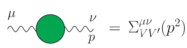
Figure 2: Vector boson two-point Green function.

whose Lorentz structure is defined with the help of two scalar functions $A$ and $B$,

$$\Sigma_{VV^{\prime}}^{\mu\nu}(p^{2})=i[A_{VV^{\prime}}(p^{2})g^{\mu\nu}+B_{VV^{\prime}}(p^{2})p^{\mu}p^{\nu}],$$ (28)

Complete prototype for bubble diagrams will be given elsewhere, while the $A$ function can be found in Diaz:2001vm .

The photon self-energy vanishes at zero momentum by virtue of gauge invariance so that after subtraction in the $\overline{DR}$ scheme contributes to the photon form-factor according to

$$\Delta F_{\gamma\chi\chi}^{vR(L)}=-e{{A_{\gamma\gamma}(s)}\over{s}}\delta_{ab}$$ (29)

where $a$ and $b$ refer to the two species of charginos produced. The photon-$Z$ mixing is also subtracted in the $\overline{DR}$ scheme and contributes to the $Z$ form-factor

$$\Delta F_{Z\chi\chi}^{vR(L)}=-e{{A_{Z\gamma}(s)}\over{s}}\delta_{ab}$$ (30)

and to photon form-factors:

$$\Delta F_{\gamma\chi\chi}^{vR(L)}={g\over{c_{W}}}O^{\prime R(L)}_{ab}{{A_{\gamma Z}(s)}\over{s-m_{Z}^{2}}}$$ (31)

The $Z$–boson self-energy is regularized with a subtraction at $s=m_{Z}^{2}$:

$$\Delta F_{Z\chi\chi}^{vR(L)}={g\over{c_{W}}}O^{\prime R(L)}_{ab}{{A_{ZZ}(s)-A_{ZZ}(m_{Z}^{2})}\over{s-m_{Z}^{2}}}$$ (32)

Another important two-point Green function is the sneutrino self energy, whose diagram is in Fig. 3

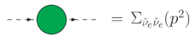
Figure 3: Sneutrino self energy.

Since it is Lorentz scalar, it is represented by only one function $A$,

$$\Sigma_{\tilde{\nu}_{e}\tilde{\nu}_{e}}(p^{2})=i[A_{\tilde{\nu}_{e}\tilde{\nu}_{e}}(p^{2})].$$ (33)

The contribution to the sneutrino form-factors is obtained after regularizing with a subtraction at $t=m_{\tilde{\nu}}^{2}$, with the following result,

$$\Delta F_{\tilde{\nu}e\chi}^{\pm}={1\over 2}gV_{b(a)1}{{A_{\tilde{\nu}\tilde{\nu}}(t)-A_{\tilde{\nu}\tilde{\nu}}(m_{\tilde{\nu}}^{2})}\over{t-m_{\tilde{\nu}}^{2}}}$$ (34)

This guarantees that the parameters $m_{Z}$ and $m_{\tilde{\nu}}$ respectively refer to the physical (pole-)masses.

The chargino two-point function can be seen in Fig. 4

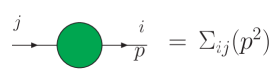
Figure 4: Chargino two-point Green function.

where the external legs correspond to any of the two charginos. Its Lorentz decomposition involves four scalar functions,

$$\Sigma_{ij}(p)=i\left[A^{+}_{ij}(p^{2})+B^{+}_{ij}(p^{2})\,\,/{\!\!\!p}\right]\frac{(1+\gamma_{5})}{2}+i\left[A^{-}_{ij}(p^{2})+B^{-}_{ij}(p^{2})\,\,/{\!\!\!p}\right]\frac{(1-\gamma_{5})}{2}.$$ (35)

The chargino self-energy and mixing contribute to form-factors in a more complicated way. Since these are external particles we have insisted that the subtractions are performed on-shell, so that the renormalized chargino fields are indeed physical fields. Details can be found in ref. Diaz:2001vm ; Diaz:1997kv .

Also embedded into form-factors are triangular diagrams, grouped into $Z\chi\chi$, $Zee$, $\gamma\chi\chi$, $\gamma ee$ and $e\chi\tilde{\nu}$ three-point functions. Form-factors are in turn easily incorporated into $Q$-charges. On the one hand, the left handed $Q$-charges that receive contributions from form-factors are,

$$\Delta Q^{L}_{1} = -\frac{g}{2c_{W}}(g^{e}_{V}+g^{e}_{A})\frac{s}{s-m_{Z}^{2}}\Delta F^{sR}_{Z\chi\chi}+e\Delta F^{sR}_{\gamma\chi\chi}$$

$$\Delta Q^{L}_{2} = -\frac{g}{2c_{W}}(g^{e}_{V}+g^{e}_{A})\frac{s}{s-m_{Z}^{2}}\Delta F^{sL}_{Z\chi\chi}+e\Delta F^{sL}_{\gamma\chi\chi}$$ (36)

$$\Delta Q^{L}_{31} = -\frac{g}{2c_{W}}(g^{e}_{V}+g^{e}_{A})\frac{s}{s-m_{Z}^{2}}\Delta F^{vR}_{Z\chi\chi}+\frac{g}{c_{W}}O^{\prime R}_{ab}\frac{s}{s-m_{Z}^{2}}\Delta F^{vL}_{Zee}+e\Delta F^{vR}_{\gamma\chi\chi}-e\delta_{ab}\Delta F^{vL}_{\gamma ee}$$

$$\Delta Q^{L}_{41} = -\frac{g}{2c_{W}}(g^{e}_{V}+g^{e}_{A})\frac{s}{s-m_{Z}^{2}}\Delta F^{vL}_{Z\chi\chi}+\frac{g}{c_{W}}O^{\prime L}_{ab}\frac{s}{s-m_{Z}^{2}}\Delta F^{vL}_{Zee}+e\Delta F^{vL}_{\gamma\chi\chi}-e\delta_{ab}\Delta F^{vL}_{\gamma ee}$$

$$-\frac{1}{2}gV_{b1}\frac{s}{t-m^{2}_{\tilde{\nu}}}\Delta F^{-}_{\tilde{\nu}e\chi}+\frac{1}{2}gV_{a1}\frac{s}{t-m^{2}_{\tilde{\nu}}}\Delta F^{+}_{\tilde{\nu}e\chi}$$

On the other hand, the right handed $Q$-charges receiving contributions from form-factors are given by,

$$\Delta Q^{R}_{1} = -\frac{g}{2c_{W}}(g^{e}_{V}-g^{e}_{A})\frac{s}{s-m_{Z}^{2}}\Delta F^{sR}_{Z\chi\chi}+e\Delta F^{sR}_{\gamma\chi\chi}$$

$$\Delta Q^{R}_{2} = -\frac{g}{2c_{W}}(g^{e}_{V}-g^{e}_{A})\frac{s}{s-m_{Z}^{2}}\Delta F^{sL}_{Z\chi\chi}+e\Delta F^{sL}_{\gamma\chi\chi}$$ (37)

$$\Delta Q^{R}_{31} = -\frac{g}{2c_{W}}(g^{e}_{V}-g^{e}_{A})\frac{s}{s-m_{Z}^{2}}\Delta F^{vR}_{Z\chi\chi}+\frac{g}{c_{W}}O^{\prime R}_{ab}\frac{s}{s-m_{Z}^{2}}\Delta F^{vR}_{Zee}+e\Delta F^{vR}_{\gamma\chi\chi}-e\delta_{ab}\Delta F^{vR}_{\gamma ee}$$

$$\Delta Q^{R}_{41} = -\frac{g}{2c_{W}}(g^{e}_{V}-g^{e}_{A})\frac{s}{s-m_{Z}^{2}}\Delta F^{vL}_{Z\chi\chi}+\frac{g}{c_{W}}O^{\prime L}_{ab}\frac{s}{s-m_{Z}^{2}}\Delta F^{vR}_{Zee}+e\Delta F^{vL}_{\gamma\chi\chi}-e\delta_{ab}\Delta F^{vR}_{\gamma ee}$$

Finally, box diagrams are directly incorporated into $Q$-charges with prototype diagrams in ref. Diaz:2001vm , and more general diagrams that will be shown elsewhere.

As opposed to bubbles and some triangular diagrams, box diagrams are UV finite. Ultraviolet divergences that occur in a few of the triangle graphs are subtracted in the $\overline{DR}$ scheme with subtraction point $Q$. Therefore, apart for the masses which are taken to be physical and the weak-mixing angle whose renormalization is described above, all other parameters are to be considered to be in the $\overline{DR}$ at the scale $Q$ in the MSSM theory. This means that the translation of the values used here to those directly extracted from experiment, such as neutral current neutrino scattering cross-sections or the measured fine-structure constant will be slightly different from that of the Standard Model (without the supersymmetric partners). For example, the treatment of the photon-$Z$ propagator system, described above, guarantees that the propagators only have poles at zero and $M_{Z}$, but there is still some remnant of photon-$Z$ mixing at these poles. We have checked numerically that the effect of a further subtraction of the photon-$Z$ mixing propagator to remove this mixing has a negligible numerical effect on our results. Furthermore, the input SUSY parameters chosen are assumed also to be the corresponding values renormalized in this scheme at the same scale. We expect the sensitivity to (reasonable) changes in renormalization scheme to be genuinely of order $\alpha_{W}/\pi$ and to have no significant effect on our numerical results. The numerical value we use for the subtraction scale in this article is $Q=1$ TeV as suggested by the SPA Project AguilarSaavedra:2005pw .

V QED Corrections

In the previous section we discussed the non-QED virtual corrections to our chargino production process. In this section we discuss the treatment of the remaining QED corrections separately because special care must be taken with IR divergences present in bubbles, triangles, and boxes involving photons. These IR divergences appear in graphs with virtual photons at low momenta of internal particles in the loop. They cancel from the cross section with corresponding IR divergences comming from real photon emission from the external fermions, i.e., bremsstrahlung Bloch:1937pw ; Kinoshita:1962ur ; Lee:1964is , which appear in both soft and collinear photons. As a remanent, large corrections proportional to $\ln(s/m^{2}_{e})$ remain, known as Leading Logarithms (these are initial state radiation corrections) and common to any of such similar process. For bremsstrahlung corrections we do not use the $Q$-charges formalism, calculating directly the corrections to the amplitude squared, using the algebraic manipulator FORM Vermaseren:2000nd .

V.1 Bremsstrahlung corrections

Diagrams contributing to the process $e^{+}e^{-}\to\tilde{\chi}^{+}\tilde{\chi}^{-}\gamma$ are depicted in Fig. 5,

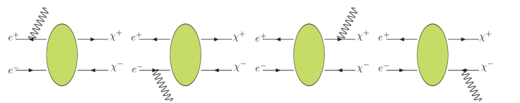
Figure 5: Real photon emission.

where the bubbles represent the three different tree-level channels ($\gamma$, $Z$, and $\tilde{\nu}_{e}$).

The total cross section $\sigma_{real}$ for a real photon emission can be written as follow,

$$\sigma_{real}=\int d\Phi_{3}\,\sum_{\lambda_{\gamma}}\,|\mathcal{M}_{real}|^{2},$$ (38)

where $d\Phi_{3}$ is the three-body phase space and $\lambda_{\gamma}$ is the photon polarization. We implement the dipole subtraction formalism introduced in Dittmaier:1999mb in order to analytically isolate the IR divergences coming from the emission of real photons, and cancel them from the also analytically extracted divergences from virtual photon diagrams. Once IR divergences are removed, the QED corrections are IR free and are calculated numerically. The dipole subtraction formalism conveniently avoids numerical problems arising when a cutoff is used to regularize the infinities.

The dipole subtraction method entails the introduction of an ad hoc auxiliary function $|\mathcal{M}_{sub}|^{2}$ which becomes equal to $\sum_{\lambda_{\gamma}}\,|\mathcal{M}_{real}|^{2}$ in the soft and collinear limits,

$$|{\cal M}_{sub}|^{2}\rightarrow\sum_{\lambda_{\gamma}}|\mathcal{M}_{real}|^{2},\ \ \mbox{as}\ \,\quad p_{i}\cdot k\rightarrow 0,$$ (39)

where $p_{i}$ are the four-momenta of the massless external fermions and $k$ is the four-moment of the photon. Adding and subtracting this function into eq. (38) we find,

$$\sigma_{real}=\int d\Phi_{3}\,(\sum_{\lambda_{\gamma}}\,|\mathcal{M}_{real}|^{2}-|\mathcal{M}_{sub}|^{2})+\int d\Phi_{3}\,|\mathcal{M}_{sub}|^{2}.$$ (40)

where the first integral is finite and is performed numerically without the serious instabilities found in cutoff methods. The second integral can be done after an analytical extraction of the IR divergences, regularized in Dittmaier:1999mb by introducing a non-zero photon mass $m_{\gamma}$, and an electron mass $m_{e}$. Once the (universal) contribution proportional to $\ln(m_{e})$ arising from initial-state radiation is removed, the soft and collinear divergent terms can be mapped into pole terms in dimensional regularization using the mappings

$$\ln\frac{m^{2}_{\gamma}}{Q^{2}}=\ln\frac{m^{2}_{e}}{Q^{2}} \to \frac{1}{\epsilon}$$

$$\ln\frac{m^{2}_{\gamma}}{Q^{2}}\ln\frac{m^{2}_{e}}{Q^{2}}-\frac{1}{2}\ln^{2}\frac{m^{2}_{e}}{Q^{2}} \to \frac{1}{\epsilon^{2}}$$ (41)

These IR divergences cancel against IR divergences from virtual diagrams (also treated by dimensional regularization).

With the process described above, the IR divergences from bremsstrahlung diagrams are,

$$\sigma^{\alpha\lambda_{1}\lambda_{2}}_{real,\,\textnormal{\scriptsize{ IR}}}=\frac{\alpha_{e}}{2\pi}\left[\frac{2}{\epsilon^{2}}+\frac{5}{\epsilon}+\frac{2}{\epsilon}\ln\left(\frac{Q^{2}}{s}\right)+\frac{2}{\epsilon}\frac{1+v^{2}}{v}\ln\frac{1-v}{1+v}+\frac{4}{\epsilon}\ln\frac{m_{\tilde{\chi}}^{2}-u}{m_{\tilde{\chi}}^{2}-t}\right]\sigma_{2\to 2}^{\alpha\lambda_{1}\lambda_{2}}$$ (42)

which as we see, are proportional to the tree-level chargino pair production cross section. In the above result, the double pole comes from simultaneous soft and collinear divergences, the simple pole not proportional to any logarithm comes from collinear divergences, while the simple pole proportional to logarithms comes from soft divergences.

V.2 Virtual Corrections

Virtual QED quantum corrections at NLO in $\alpha_{e}$ are given by,

$$\sigma^{\alpha\lambda_{1}\lambda_{2}}_{virt}=\frac{\alpha_{e}}{4\pi}\int d\Phi_{2}\ 2\mathbb{R}e\langle({\cal M}_{2\to 2}^{\alpha\lambda_{1}\lambda_{2}})^{*}{\cal M}_{virt}^{\alpha\lambda_{1}\lambda_{2}}\rangle$$ (43)

where ${\cal M}_{2\to 2}^{\alpha\lambda_{1}\lambda_{2}}$ is the tree level amplitude, ${\cal M}_{virt}^{\alpha\lambda_{1}\lambda_{2}}$ contains all QED virtual corrections, and the photon coupling to fermions is factor out in $\alpha_{e}/(4\pi)$. In $\overline{DR}$, the IR divergent contributions from virtual QED correction can be written as,

$$\sigma^{\alpha\lambda_{1}\lambda_{2}}_{virt,\,\textnormal{\scriptsize{ IR}}}=-\frac{\alpha_{e}}{2\pi}\left[\frac{2}{\epsilon^{2}}+\frac{5}{\epsilon}+\frac{2}{\epsilon}\ln\left(\frac{Q^{2}}{s}\right)+\frac{2}{\epsilon}\frac{1+v^{2}}{v}\ln\frac{1-v}{1+v}+\frac{4}{\epsilon}\ln\frac{m_{\tilde{\chi}}^{2}-u}{m_{\tilde{\chi}}^{2}-t}\right]\sigma_{2\to 2}^{\alpha\lambda_{1}\lambda_{2}}$$ (44)

where details will be given elsewhere. Clearly from eqs. (42) and (44), virtual and real IR divergences cancel each other.

VI Numerical Results

As a working example we concentrate on the mSUGRA Focus Point known as SPS2 Allanach:2002nj . This scenario is characterized by,

$m_{0}=1450$ GeV,

$m_{1/2}=300$ GeV,

$A_{0}=0$ GeV,

$\tan\beta=10$,

$\mu>0$

and we use the code ISAJET for the running from GUT to weak scale Baer:1999sp . The low energy soft parameters calculated this way are fed into our code. The integration over phase space is performed with a MonteCarlo technique. Some relevant low energy parameters and masses are shown in the following table,

parameters (GeV)	masses (GeV)
$M_{1}=121.9$	$m_{\tilde{\chi}_{1}^{+}}^{0}=172.1$
$M_{2}=235.7$	$m_{\tilde{\chi}_{2}^{+}}^{0}=297.0$
$\mu=222.2$	$m_{\tilde{\chi}^{0}_{1}}=111.5$
	$m_{\tilde{\nu}_{e}}=1454$

where the charginos, neutralino, and sneutrino masses are given at tree-level. We correct the chargino masses at one-loop, and in order to compare the corrected cross section without moving the threshold, we define a tree-level scenario where the values of $M_{2}$ and $\mu$ are tuned such that this tree-level masses are equal to the one-loop corrected chargino masses. These new tree-level parameters and one-loop corrected chargino masses are in the following table,

parameters (GeV)	masses (GeV)
$M_{2}^{0}=242.9$	$m_{\tilde{\chi}_{1}^{+}}=173.7$
$\mu^{0}=219.7$	$m_{\tilde{\chi}_{2}^{+}}=300.0$

We report below only on production cross sections of light charginos, with a mass of $m_{\chi^{+}_{1}}=173.7$ GeV as shown on the table.

As we mentioned before, the renormalization scale we use is $Q=1$ TeV motivated by the SPA Project AguilarSaavedra:2005pw . Electroweak observables $\sin^{2}\theta_{W}^{\overline{MS}}(m_{z})$ and $\alpha(m_{Z})$ mentioned in section II must be run up to the scale $Q=1$ TeV. We find $\sin^{2}\theta_{W}^{\overline{MS}}(Q)=0.2395$ and $\alpha(Q)=1/125$, which translates into $g(Q)=0.6479$ and $g^{\prime}(Q)=0.3636$, as reported in AguilarSaavedra:2005pw .

We separate the corrections in the following way: by “MSSM” corrections we mean all loops that do not include photons, by “QED” corrections we mean all loops including photons (virtual QED) plus all bremsstrahlung diagrams, and by “$\ell\ell$” we mean the leading logarithms, which are universal to all this kind of processes.

Our definition for the “$\ell\ell$” contribution is,

$$\sigma_{\ell\ell}^{\alpha\lambda_{1}\lambda_{2}}=\frac{\alpha}{\pi}\ln\left(\frac{s}{m_{e}^{2}}\right)\int_{0}^{1}\,dx\,\frac{1+x^{2}}{1-x}\left[\int d\Phi_{2}(x)\Big{|}{\cal M}_{2\rightarrow 2}^{\alpha\lambda_{1}\lambda_{2}}(xp)\Big{|}^{2}-\int d\Phi_{2}(1)\Big{|}{\cal M}_{2\rightarrow 2}^{\alpha\lambda_{1}\lambda_{2}}(p)\Big{|}^{2}\right]$$ (45)

where the term $\ln\left(\frac{s}{m_{e}^{2}}\right)$ is precisely the large logarithm that gives the name to the whole leading logarithm contribution. The function $(1+x^{2})/(1-x)$ is the splitting function, which is related to the probability of finding an electron or a positron with a momentum $xp$ before the emission of a photon, which takes a momentum $(1-x)p$. The differential $d\Phi_{2}(x)$ is the 2-body phase space with one incoming 4-momentum multiplied by $x$, which translates into $s\rightarrow xs$.

VI.1 Unpolarized Total Cross Section

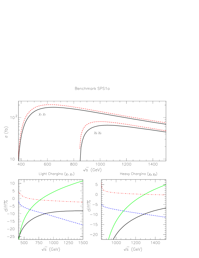
Figure 6: Unpolarized total cross section as a function of $\sqrt{s}$ for the SPS1a scenario. In the upper frame we compare the tree-level (red-dashed), with full NLO (black-solid). In the lower frames, the different curves correspond to full NLO corrected (black solid), MSSM (blue dashes), QED (red dot-dash), and $\ell\ell$ (green solid).

We start by comparing our unpolarized results with the ones reported in Oller:2005xg . In this reference the result for NLO corrections to the unpolarized cross section was reported for the scenario known as SPS1a. In that case, complete NLO quantum corrections are very large and negative, strengthen by a large contribution from sneutrinos, due to a small sneutrino mass and large sneutrino-neutrino-electron coupling. Our predictions for the total NLO cross section for light charginos in SPS1a, whose corrections vary from $-27\%$ at $\sqrt{s}=400$ GeV, to $-7\%$ at $\sqrt{s}=1400$ GeV, are in reasonable agreement with the ones reported in Oller:2005xg within $\pm 2\%$, as can be seen in the lower-left frame of our Fig. 6. Similarly, the total NLO cross section for heavy charginos vary from $-22\%$ at $\sqrt{s}=980$ GeV to $-8\%$ at $\sqrt{s}=1400$ GeV, and they are also in agreement within $\pm 2\%$ with Oller:2005xg .

Of course, the magnitude of quantum corrections depends on the supersymmetric benchmark chosen. We already mentioned that our working scenario is benchmark SPS2, also known as Focus Point. In Fig. 7 we show the one-loop unpolarized total cross section as a function of the center of mass energy $\sqrt{s}$. In the upper plot we have the total cross section in the Born approximation (red dash line), and the NLO corrected total cross section (black solid line), for light and heavy charginos. We see that in this scenario NLO corrections to the total cross section for light charginos, change sign at $\sqrt{s}\approx 1250$ GeV, while for heavy charginos the correction is always negative in region shown in the graph.

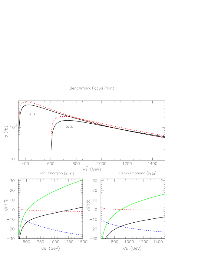
Figure 7: Unpolarized total cross section as a function of $\sqrt{s}$. The different curves correspond to full NLO corrected (black solid), MSSM (blue dashes), QED (red dot-dash), and $\ell\ell$ (green solid).

In the lower frames of Fig. 7 we show details of the NLO corrections, as in the previous figure. The magnitude of the corrections rise sharply as the energy approaches the threshold, although this percentage correction acts on a total cross section that approaches zero in this limit.

We note that the corrections in the case of Focus point SPS2 considered in this paper, are considerable different from those of benchmark SPS1a. The MSSM correction (excluding the pure QED corrections) are consistently lower (negative) in the case of SPS2. The major difference comes form the l.l. part of the QED corrections which, at high energies, are nearly three times as large as the case of SPS1a. This substantial difference is in turn dominated by a difference in the initial radiation correction to the sneutrino exchange part of the amplitude. For SPS2 the sneutrino mass is much larger than for SPS1a, so that its contribution to the tree-level differential cross-section is very insensitive to scattering angle, and negligible in front of s-channel contributions. On the other hand, sneutrino contribution in SPS1a scenario is large, and interferes destructively with s-channel contributions. All in all this leads to a light chargino total correction for the SPS2 point which is positive for $\sqrt{s}\,>\,$ 1250 GeV, whereas for SPS1a, the total correction remains negative.

VI.2 Polarized Differential Cross Sections

In this section we show our results for one-loop corrected differential cross sections for the production of light charginos with definite helicity from polarized electron positron collisions, in the Focus Point SPS2 scenario. We choose to show our results for the differential cross sections as a function of $\chi^{+}_{1}$ transverse momentum $p_{T}$ (rather than the scattering angle) defined as,

$$p_{T}^{2}=\frac{4}{s}(p_{1}\cdot k_{2})(p_{2}\cdot k_{2})-m_{\tilde{\chi}_{1}^{+}}^{2}$$ (46)

where the center of mass energy is $\sqrt{s}=1000$ GeV. In the case there is no photon in the final state, this reduces to $p_{T}=\sqrt{s}\,v\sin\theta/2$, where $v$ and $\theta$ are $\chi^{+}_{1}$ velocity and scattering angle.

The differential cross section we are working with is related to the differential cross section as a function of $\cos\theta$ in the following way,

$$\frac{d\sigma}{dp_{T}}=\frac{2\tan\theta}{\sqrt{s}\,v}\frac{d\sigma}{d\cos\theta}$$ (47)

which partly explains the tendency for the cross section ${d\sigma}/{dp_{T}}$ to grow with $p_{T}$, as we go from $\theta=0$ to $\theta=\pi/2$.

In the following six figures we show quantum corrections to polarized chargino production cross section as a function of transverse momentum. All of these figures have the same structure and differ in the chargino helicities and the electron polarization. In all plots we show $p_{T}>100$ GeV because it is the most interesting region, with larger cross sections and better chances of differentiation from background.

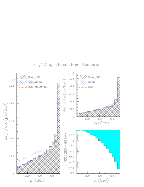
Figure 8: $d\sigma_{L}^{+-}/dp_{T}$ as a function of $p_{T}$ in the Focus Point scenario within mSUGRA.

In Fig. 8 we have $d\sigma_{L}^{+-}/dp_{T}$, i.e., for a chargino with positive helicity, an antichargino with negative helicity, and a left handed electron (right handed positron). On the left we have the differential cross section as a function of $p_{T}$, where we compare the born approximation, the one-loop corrected cross section including MSSM and QED corrections, and the corrected cross section including MSSM, QED, and leading logarithms. QED+MSSM corrections are moderate and negative, varying between -1% and -18%, as can be seen also in the lower right frame. Leading logarithms are very large, and increase the differential cross section even more, except at large $p_{T}$, where $\ell\ell$ are negative. The largest positive corrections are obtained for low transverse momentum, $p_{T}\sim 100$ GeV, while the largest negative corrections appear at $p_{T}\sim 440$ GeV. This choice for the chargino helicities and electron polarization gives the highest values for the differential cross section, varying between 0.2 and 2.1 fb/GeV. In the upper right frame we show the MSSM and QED corrections separately from each other, and compared with the Born approximation. We see that the QED corrections (not including leading logarithms) are smaller than 1%.

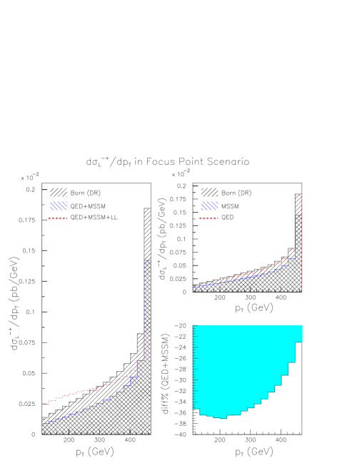
Figure 9: $d\sigma_{L}^{-+}/dp_{T}$ as a function of $p_{T}$ in the Focus Point scenario within mSUGRA.

In Fig. 9 we have $d\sigma_{L}^{-+}/dp_{T}$, which corresponds to the case with both chargino helicities reversed with respect to the previous case. The differential cross section is comparable, varying between 0.1 and 1.4 fb/GeV, as we see in the left frame. In the lower right frame we observe that QED+MSSM corrections are larger in magnitude than the previous case, and also negative. Note that here the relative magnitude of the corrections decrease with $p_{T}$, as opposed to the previous case, where they increase. Another difference with the previous case is that QED corrections are larger, but smaller in magnitude than MSSM corrections, as seen in the upper-right frame. This is a case where QED quantum corrections should not be neglected. The Leading Logarithms are usually positive, but become negative at large $p_{T}$, owing to the fact that at large $p_{T}$, $x$ is required to be larger than $4p_{T}^{2}/s$, thereby reducing the $x$-dependent phase-space factor $\Phi_{2}(x)$ in eq.(45). All the above differences between the corrections to $\sigma_{L}^{+-}$ and $\sigma_{L}^{-+}$ are interesting manifestations of the parity violation properties of the MSSM.

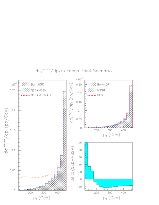
Figure 10: $d\sigma_{L}^{++,--}/dp_{T}$ as a function of $p_{T}$ in the Focus Point scenario within mSUGRA.

In Fig. 10 we see the equal chargino helicity production cross section. CP invariance, which we assume, enforces the equality of $d\sigma_{L}^{++}/dp_{T}$ and $d\sigma_{L}^{--}/dp_{T}$, and it serves as a check of our calculations. This cross section is much smaller, varying from less than 0.001 fb/GeV at low $p_{T}$ up to almost 0.2 fb/GeV at large $p_{T}$. In the lower-right frame we see that QED+MSSM quantum corrections are negative at large $p_{T}$, and positive at low $p_{T}$, although in that case they are correcting a cross section which is already very small at tree-level. From the upper-right frame we learn that QED corrections are smaller than MSSM corrections, however they cannot be neglected at medium values for $p_{T}$. Leading logarithms are comparatively large, but in absolute terms they are smaller than in the different helicity cases.

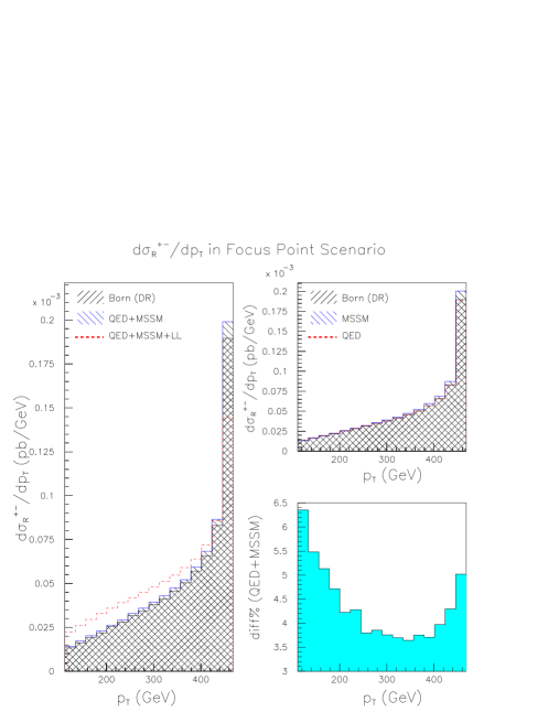
Figure 11: $d\sigma_{R}^{+-}/dp_{T}$ as a function of $p_{T}$ in the Focus Point scenario within mSUGRA.

In the next three figures we plot differential cross sections where right handed electrons collide with left handed positrons. These cross sections are noticeably smaller than the case with left handed electrons. The reason is an accidental cancellation between $Z$ and photon contributions in the amplitude already present at tree-level, as it was explained before. In Fig. 11 we have $d\sigma_{R}^{+-}/dp_{T}$, which varies from 0.01 to 0.2 fb/GeV as $p_{T}$ grows from 100 GeV up to 468.8 GeV, which is the maximum value for $p_{T}$. QED+MSSM corrections vary slowly between $3\%$-$6\%$, as seen in the lower-right frame. Nevertheless, from the upper-right frame we see that most of these corrections come from MSSM loops and QED can be neglected. In addition, leading logarithms can be seen in the left frame, and they are large and positive with the exception of very large $p_{T}$ where they can be negative.

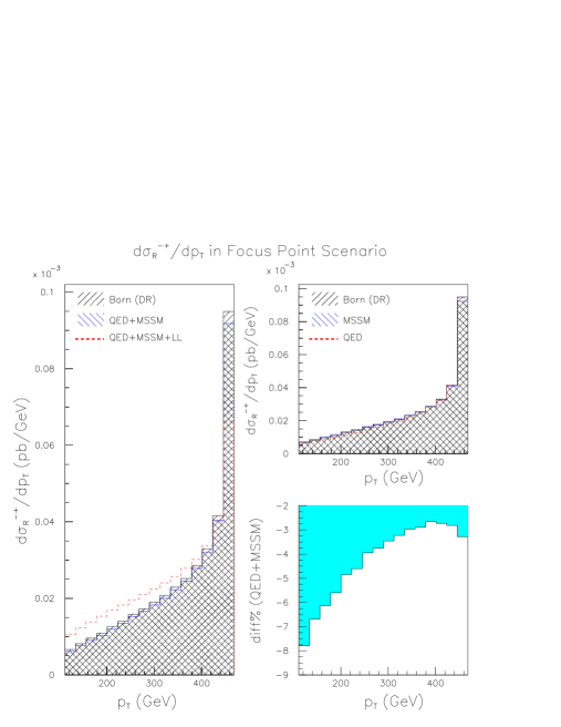
Figure 12: $d\sigma_{R}^{-+}/dp_{T}$ as a function of $p_{T}$ in the Focus Point scenario within mSUGRA.

In Fig. 12 we have $d\sigma_{R}^{-+}/dp_{T}$, which is a factor 1/2 smaller than the previous one. Quantum corrections corresponding to QED+MSSM are larger, between $-3\%$ and $-8\%$, and interestingly enough they have different sign than the case with opposite chargino helicities, thus they cancel and not add to each other as in the case for left handed electrons. Nevertheless, these large corrections for right handed electrons act on a 10 times smaller cross section compared with left handed electrons. If electrons are not $100\%$ polarized (as expected) the pure right handed cross section will be diluted by the left handed cross section. We see from the upper-right frame that the QED corrections are of the same order than MSSM ones, and non-negligible. Leading logarithms are large, positive for small $p_{T}$ and negative for high $p_{T}$.

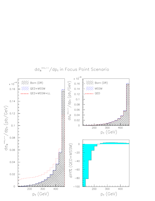
Figure 13: $d\sigma_{R}^{++,--}/dp_{T}$ as a function of $p_{T}$ in the Focus Point scenario within mSUGRA.

Finally, in Fig. 13 we have the equal chargino helicities production cross section $d\sigma_{R}^{++}/dp_{T}=d\sigma_{R}^{--}/dp_{T}$ for the case of right handed electrons and left handed positrons. This cross section is extremely small, never bigger than 0.02 fb/GeV. Quantum corrections are very large at small $p_{T}$, but with cross sections so small that the chance to be observed is minimal. We include it for completness.

VII Conclusions

We have calculated the complete one-loop quantum corrections to the differential cross section for chargino production in electron positron collisions, at 1 TeV center of mass energy, relevant for the future International Linear Collider. In the analysis we have included the electron and positron polarization, as well as the chargino helicities.

We organize the non-QED corrections calculating the helicity amplitudes, and regularizing the ultraviolet divergences with Dimensional Regularization. Our renormalization scheme includes on shell masses and $\overline{DR}$ running couplings. In addition, we use the dipole subtraction formalism in Bremsstrahlung contributions to cancel analytically soft and collinear divergences, with infrared divergences from virtual QED corrections. The well known leading logarithms remain, and we isolate them in order to better understand quantum corrections.

We show numerical results for the Focus Point scenario in mSUGRA. The dipole subtraction formalism is designed to handle analytically the divergences, therefore the use of infrared cut-offs becomes unnecessary, making the calculation numerically stable. We find important quantum corrections for differential cross sections with definite chargino helicities. The substantial differences in the NLO corrections depending on the helicities of the charginos and of the initial leptons, show that the rich structure of the MSSM - in particular the parity violating properties - can be investigated, firstly by polarization of the incoming electron/proton beam and secondly by determining (through the angular distributions of the decay products) the helicities of the charginos produced gudrid ; Bernreuther:2001rq . Since charginos are unstable, the full potential of this work will be fulfilled when similar radiative corrections are included for the chargino decay, and the spin correlations between production and decay are evaluated. Large corrections of the order of -18% and -35% are obtained for the largest cross sections, $d\sigma_{L}^{-+}/dp_{T}$ and $d\sigma_{L}^{+-}/dp_{T}$. They are large enough to making it necessary to include them in any analysis for the ILC.

- (1) H. E. Haber and G. L. Kane, Phys. Rept. 117, 75 (1985).
- (2) G. Abbiendi et al. [OPAL Collaboration], Eur. Phys. J. C 35, 1 (2004) [arXiv:hep-ex/0401026].
- (3) J. Abdallah et al. [DELPHI Collaboration], Eur. Phys. J. C 31, 421 (2004) [arXiv:hep-ex/0311019].
- (4) A. Heister et al. [ALEPH Collaboration], Phys. Lett. B 533, 223 (2002) [arXiv:hep-ex/0203020].
- (5) M. Acciarri et al. [L3 Collaboration], Phys. Lett. B 472, 420 (2000) [arXiv:hep-ex/9910007].
- (6) T. Aaltonen et al. [CDF Collaboration], Phys. Rev. Lett. 101, 251801 (2008) [arXiv:0808.2446 [hep-ex]].
- (7) V. M. Abazov et al. [D0 Collaboration], arXiv:0901.0646 [hep-ex].
- (8) G. Polesello, J. Phys. G 30 (2004) 1185.
- (9) U. Blumenschein,
- (10) J. Kalinowski, arXiv:hep-ph/9905558.
- (11) D. Pierce and A. Papadopoulos, Phys. Rev. D 50, 565 (1994)
- (12) H. Eberl, M. Kincel, W. Majerotto and Y. Yamada, Phys. Rev. D 64, 115013 (2001) [arXiv:hep-ph/0104109].
- (13) T. Fritzsche and W. Hollik, Eur. Phys. J. C 24, 619 (2002) [arXiv:hep-ph/0203159].
- (14) R. Schofbeck and H. Eberl, Eur. Phys. J. C 53, 621 (2008) [arXiv:0706.0781 [hep-ph]].
- (15) M. A. Diaz, S. F. King and D. A. Ross, Nucl. Phys. B 529, 23 (1998) [arXiv:hep-ph/9711307].
- (16) J. R. Ellis, T. Falk, G. Ganis, K. A. Olive and M. Schmitt, Phys. Rev. D 58, 095002 (1998)
- (17) W. Oller, H. Eberl and W. Majerotto, Phys. Rev. D 71, 115002 (2005)
- (18) W. Kilian, J. Reuter and T. Robens, Eur. Phys. J. C 48, 389 (2006)
- (19) T. Robens, arXiv:hep-ph/0610401.
- (20) T. Blank and W. Hollik, arXiv:hep-ph/0011092.
- (21) S. Kiyoura, M. M. Nojiri, D. M. Pierce and Y. Yamada, Phys. Rev. D 58, 075002 (1998) [arXiv:hep-ph/9803210].
- (22) S. Hao, H. Liang, M. Wen-Gan, Z. Ren-You, J. Yi and G. Lei, Phys. Rev. D 73, 055002 (2006) [arXiv:hep-ph/0602089].
- (23) J. Fujimoto, T. Ishikawa, Y. Kurihara, M. Jimbo, T. Kon and M. Kuroda, Phys. Rev. D 75, 113002 (2007).
- (24) R. Y. Zhang, W. G. Ma and L. H. Wan, J. Phys. G 28, 169 (2002) [arXiv:hep-ph/0111124].
- (25) M. A. Diaz and D. A. Ross, JHEP 0106, 001 (2001) [arXiv:hep-ph/0103309].
- (26) M. A. Diaz, S. F. King and D. A. Ross, Phys. Rev. D 64, 017701 (2001) [arXiv:hep-ph/0008117].
- (27) M. A. Diaz and D. A. Ross, arXiv:hep-ph/0205257.
- (28) H. Baer, M. A. Diaz, M. A. Rivera and D. A. Ross, arXiv:hep-ph/0210444.
- (29) G. Moortgat-Pick, H. Fraas, Phys. Rev. D 59, 015016 (1999); G. Moortgat-Pick, H. Fraas, A. Bartl, W. Majerotto, Eur. Phys. J. C7, 113 (1999); G. Moortgat-Pick, H. Fraas, A. Bartl, W. Majerotto, Eur. Phys. J. C9, 521 (1999), Erratum-ibid. C9, 549 (1999); G. Moortgat-Pick, A. Bartl, H. Fraas, W. Majerotto, Eur. Phys. J. C18, 379 (2000).
- (30) S. Dittmaier, Nucl. Phys. B 565, 69 (2000)
- (31) W. M. Yao et al. [Particle Data Group], J. Phys. G 33 (2006) 1.
- (32) J. A. Aguilar-Saavedra et al., Eur. Phys. J. C 46, 43 (2006) [arXiv:hep-ph/0511344].
- (33) G. Abbiendi et al. [OPAL Collaboration], Eur. Phys. J. C 19, 587 (2001) [arXiv:hep-ex/0012018]; P. Abreu et al. [DELPHI Collaboration], Eur. Phys. J. C 16 (2000) 371; M. Acciarri et al. [L3 Collaboration], Eur. Phys. J. C 16, 1 (2000) [arXiv:hep-ex/0002046]; R. Barate et al. [ALEPH Collaboration], Eur. Phys. J. C 14, 1 (2000).
- (34) F. Bloch and A. Nordsieck, Phys. Rev. 52, 54 (1937).
- (35) T. Kinoshita, J. Math. Phys. 3, 650 (1962).
- (36) T. D. Lee and M. Nauenberg, Phys. Rev. 133, B1549 (1964).
- (37) H. Baer, F. E. Paige, S. D. Protopopescu and X. Tata, arXiv:hep-ph/0001086.
- (38) J. A. M. Vermaseren, “New Features Of FORM,” arXiv:math-ph/0010025.
- (39) B. C. Allanach et al., in Proc. of the APS/DPF/DPB Summer Study on the Future of Particle Physics (Snowmass 2001) ed. N. Graf, Eur. Phys. J. C 25, 113 (2002).
- (40) W. Bernreuther, A. Brandenburg, Z. G. Si and P. Uwer, Phys. Rev. Lett. 87, 242002 (2001) [arXiv:hep-ph/0107086].