Criticality and heterogeneity in the solution space of random constraint satisfaction problems

Abstract

Random constraint satisfaction problems are interesting model systems for spin-glasses and glassy dynamics studies. As the constraint density of such a system reaches certain threshold value, its solution space may split into extremely many clusters. In this work we argue that this ergodicity-breaking transition is preceded by a homogeneity-breaking transition. For random $K$-SAT and $K$-XORSAT, we show that many solution communities start to form in the solution space as the constraint density reaches a critical value $\alpha_{cm}$, with each community containing a set of solutions that are more similar with each other than with the outsider solutions. At $\alpha_{cm}$ the solution space is in a critical state. The connection of these results to the onset of dynamical heterogeneity in lattice glass models is discussed.

I Introduction

Random constraint satisfaction problems (CSPs) have attracted a lot of research interest from the statistical physics community in recent yearsHartmann-Weigt-2005 ; Mezard-Montanari-2009 ; Monasson-Zecchina-1996 ; Mezard-etal-2002 . These are model systems for understanding typical-case computational complexity of nonpolynomial-complete problems in computer science, some of them have also important applications in modern coding systems, such as the low-density-parity-check codes. The energy landscape of a nontrivial random CSP problem is usually very complicated, similar to those of spin-glassesMezard-Parisi-2001 ; Mezard-Parisi-2003 and lattice glass modelsBiroli-Mezard-2002 ; Darst-Reichman-Biroli-2009 . Therefore understanding the configuration space property of random CSPs is also very helpful for developing new insights for spin-glasses, glassy dynamics, and the jamming phenomena of colloids and granular systems.

As the density $\alpha$ of constraints increases, the solution space of a CSP will experience a series of phase transitionsKrzakala-etal-PNAS-2007 . One of them is the clustering transition at certain threshold constraint density $\alpha_{d}$, where the solution space splits into exponentially many isolated solution clusters or Gibbs states. This ergodicity-breaking transition has very significant consequences for glassy dynamicsMontanari-Semerjian-2006 ; Mezard-Montanari-2006 and stochastic local search processesKrzakala-Kurchan-2007 ; Alava-etal-2008 ; Zhou-2009 . Numerical simulationsZhou-Ma-2009 further suggested that, before ergodicity of the solution space is broken, the solution space has already been non-homogeneous, with the formation of many solution communities. In this paper we determine the critical constraint density $\alpha_{cm}$ for the solution space of a random CSP to become heterogeneous. We find that $\alpha_{cm}<\alpha_{d}$, and that at $\alpha=\alpha_{cm}$ the solution space is in a critical state, in which the boundaries between different solution communities of the solution space disappears, while at $\alpha>\alpha_{cm}$ the solution space contains many well-formed solution communities.

Heterogeneity of the configuration space of a complex system can cause heterogeneity in the dynamics of this system. The results of this work may be helpful for understanding more quantitatively the nature of dynamical heterogeneity in supercooled liquidsEdiger-2000 ; Glotzer-2000 ; Cavagna-2009 and lattice glass modelsDarst-Reichman-Biroli-2009 ; Biroli-Mezard-2002 .

II Theory

A constraint satisfaction formula has $N$ vertices ($i,j,k,\ldots$) and $M$ constraints ($a,b,c,\ldots$), with constraint density $\alpha\equiv M/N$. A configuration of the model is denoted by $\vec{\sigma}\equiv\{\sigma_{1},\sigma_{2},\ldots,\sigma_{N}\}$, where $\sigma_{i}=\pm 1$ is the spin state of vertex $i$. Each constraint $a$ represents a multi-spin interaction among a subset (denoted as $\partial a$) of vertices, and its energy $E_{a}$ is either zero (constraint being satisfied) or positive (unsatisfied). For example, $E_{a}$ may be expressed as

$$E_{a}=1-J_{a}\prod\limits_{i\in\partial a}\sigma_{i}$$ (1)

where $J_{a}=+1$ or $-1$ depending on the constraint $a$. The total energy of a spin configuration $\vec{\sigma}$ is the sum of individual constraint energies, $E(\vec{\sigma})=\sum_{a=1}^{M}E_{a}$.

A solution of a constraint satisfaction formula is a spin configuration of zero total energy. The whole set of solutions for a given energy function $E(\vec{\sigma})$ is denoted as $\mathcal{S}$ and referred to as the solution space. The energy landscape of a CSP may be very complex and its ground-state degeneracy usually is extremely high. To investigate the structure of a solution space $\mathcal{S}$, we define a partition function as

$$Z(x)=\sum\limits_{\vec{\sigma}^{1}\in\mathcal{S}}\sum\limits_{\vec{\sigma}^{2}\in\mathcal{S}}\exp\Bigl{(}x\sum\limits_{i=1}^{N}\sigma_{i}^{1}\sigma_{i}^{2}\Bigr{)}\ ,$$ (2)

where $x$ is a binding field. Each solution pair $(\vec{\sigma}^{1},\vec{\sigma}^{2})$ contributes a term $\exp[Nxq(\vec{\sigma}^{1},\vec{\sigma}^{2})]$ to $Z(x)$, with $q(\vec{\sigma}^{1},\vec{\sigma}^{2})\equiv(1/N)\sum_{i=1}^{N}\sigma_{i}^{1}\sigma_{i}^{2}$ being the solution-solution overlap. We introduce an entropy density $s(q)$ by expressing the total number $\mathcal{N}(q)$ of solution-pairs with overlap $q$ as $\mathcal{N}(q)=\exp[Ns(q)]$. Then Eq. (2) is re-written as

$$Z(x)=\sum\limits_{q}\exp\Bigl{[}N\bigl{(}s(q)+xq\bigr{)}\Bigr{]}\ .$$ (3)

The free entropyMezard-Montanari-2009 $\Phi(x)$ of the system is related to the partition function by $\Phi(x)\equiv\ln Z(x)$ In the thermodynamic limit of $N\rightarrow\infty$, the free entropy density $\phi(x)\equiv\Phi(x)/N$ is related to the entropy density $s(q)$ by

$$\phi(x)=\max\limits_{q\in[-1,1]}\Bigl{[}s(q)+xq\Bigr{]}=s\bigl{(}\overline{q}(x)\bigr{)}+x\overline{q}(x)\ .$$ (4)

In Eq. (4), $\overline{q}(x)$ is the overlap value at which the function $s(q)+xq$ achieves the global maximal value. $\overline{q}(x)$ is also the mean value of solution-solution overlaps under the binding field $x$.

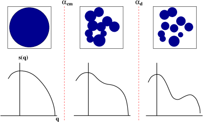
Figure 1: Evolution of the solution space $\mathcal{S}$ of a constrained spin system: At low constraint density $\alpha$ (left panel), $\mathcal{S}$ is homogeneous and the solution-pair entropy density $s(q)$ is a concave function of the overlap $q$. Solution communities start to form as $\alpha$ exceeds a threshold value $\alpha_{cm}$ (middle panel); $\mathcal{S}$ then becomes heterogeneous and the function $s(q)$ changes to be non-concave. An ergodicity-breaking transition occurs as $\alpha$ reaches a larger threshold value $\alpha_{d}$ (right panel), where the solution communities separate into different solution clusters and $s(q)$ becomes non-monotonic. As $\alpha$ further increases, solution-pairs with intermediate overlap values may disappear completely, and then $s(q)$ is not defined for these intermediate overlap values.

At $x=0$, the maximum of Eq. (4) is achieved at $\overline{q}(0)=q_{0}$, the most probable solution-pair overlap value; at the other limit of $x\rightarrow\infty$, $\overline{q}(\infty)=1$. If the entropy density $s(q)$ is a concave function of $q\in[q_{0},1]$ (Fig. 1, left panel), then for each $x>0$ there is only one mean overlap value $\overline{q}$, and $\overline{q}(x)$ changes smoothly with $x$. On the other hand, if $s(q)$ is non-concave in $q\in[q_{0},1]$ (Fig. 1, middle and right panel), then at certain value $x^{*}$ of the binding field, there are two different mean overlap values, and the value of $\overline{q}(x)$ changes discontinuously at $x=x^{*}$ (a field-induced first-order phase-transition). In this work, we exploit this correspondence between the non-concavity of $s(q)$ and the discontinuity of $\overline{q}(x)$ to determine the threshold constraint density $\alpha_{cm}$ at which the solution space $\mathcal{S}$ becomes heterogeneous. Many solution communities can be identified in a heterogeneous solution space $\mathcal{S}$Zhou-Ma-2009 . Each solution community contains a set of solutions which are more similar with each other than with the solutions of other communities. These differences of intra- and inter-community overlap values and the relative sparseness of solutions at the boundaries between solution communities cause the non-concavity of $s(q)$.

III Application to the random $K$-SAT problem

We begin with the random $K$-SAT, a prototypical CSPMonasson-Zecchina-1996 ; Mezard-etal-2002 ; Krzakala-etal-PNAS-2007 . In a random $K$-SAT formula, the number of vertices in the set $\partial a$ of each constraint $a$ is fixed to $K$, and these $K$ different vertices are randomly chosen from the whole set of $N$ vertices. Depending on the spins of these $K$ vertices, the energy of a constraint $a$ is either zero or unity:

$$E_{a}=\prod\limits_{i\in\partial a}\frac{1-J_{a}^{i}\sigma_{i}}{2}\ ,$$ (5)

where $J_{a}^{i}=\pm 1$ with equal probability. The solution space $\mathcal{S}$ of a large random $K$-SAT formula is non-empty if the constraint density $\alpha$ is less than a satisfiability threshold $\alpha_{s}(K)$Mertens-etal-2006 . Before $\alpha_{s}(K)$ is reached, $\mathcal{S}$ has an ergodicity-breaking transition at a clustering transition point $\alpha_{d}(K)$, where it breaks into extremely many solution clustersKrzakala-etal-PNAS-2007 . We will see shortly that this clustering transition is preceded by another transition at $\alpha=\alpha_{cm}(K)$, where $\mathcal{S}$ starts to be heterogeneous as many solution communities are formed.

We use the replica-symmetric cavity method of statistical mechanicsMezard-Parisi-2001 to calculate the mean overlap value $\overline{q}(x)$ at $\alpha<\alpha_{d}(K)$. As the partition function Eq. (2) is a summation over pairs of solutions $(\vec{\sigma}^{1},\vec{\sigma}^{2})$, the state of each vertex is a pair of spins $(\sigma,\sigma^{\prime})$. Consider a vertex $i$ which is involved in a constraint $a$, $i\in\partial a$. The following two cavity probabilities $p_{i\rightarrow a}(\sigma_{i},\sigma_{i}^{\prime})$ and $\hat{p}_{a\rightarrow i}(\sigma_{i},\sigma_{i}^{\prime})$ are defined: $p_{i\rightarrow a}(\sigma_{i},\sigma_{i}^{\prime})$ is the probability that, in the absence of constraint $a$, vertex $i$ has spin value $\sigma_{i}$ in solution $\vec{\sigma}^{1}$ and value $\sigma_{i}^{\prime}$ in solution $\vec{\sigma}^{2}$; and $\hat{p}_{a\rightarrow i}(\sigma_{i},\sigma_{i}^{\prime})$ is the probability that the constraint $a$ is satisfied conditional to vertex $i$ being in state $(\sigma_{i},\sigma_{i}^{\prime})$. One can write down the following iterative equations:

$$\hat{p}_{a\rightarrow i}(\sigma_{i},\sigma_{i}^{\prime}) = 1-\delta_{\sigma_{i}}^{-J_{a}^{i}}\prod\limits_{j\in\partial a\backslash i}\Bigl{[}\sum_{\sigma}p_{j\rightarrow a}(-J_{a}^{j},\sigma)\Bigr{]}-\delta_{\sigma_{i}^{\prime}}^{-J_{a}^{i}}\prod\limits_{j\in\partial a\backslash i}\Bigl{[}\sum_{\sigma}p_{j\rightarrow a}(\sigma,-J_{a}^{j})\Bigr{]}$$ (6)

$$+\delta_{\sigma_{i}}^{-J_{a}^{i}}\delta_{\sigma_{i}^{\prime}}^{-J_{a}^{i}}\prod\limits_{j\in\partial a\backslash i}p_{j\rightarrow a}(-J_{a}^{j},-J_{a}^{j})\ ,$$

$$p_{i\rightarrow a}(\sigma_{i},\sigma_{i}^{\prime}) = Ce^{x\sigma_{i}\sigma_{i}^{\prime}}\prod\limits_{b\in\partial i\backslash a}\hat{p}_{b\rightarrow i}(\sigma_{i},\sigma_{i}^{\prime})\ ,$$ (7)

where $\delta_{m}^{n}$ is the Kronecker symbol, $C$ is a normalization constant, and $\partial i$ denotes the set of constraints that vertex $i$ is associated with. The probability $p_{i}(\sigma_{i},\sigma_{i}^{\prime})$ of vertex being in the spin-pair state $(\sigma_{i},\sigma_{i}^{\prime})$ has the same expression as Eq. (7) but with $\partial i\backslash a$ replaced by $\partial i$. In writing down the above cavity equations, we have applied the Bethe-Peierls factorization approximation of cavity probabilities, which corresponds to the replica-symmetric cavity theoryMezard-Parisi-2001 ; Mezard-Montanari-2006 . For each vertex $i$ the probabilities $p_{i}$ and $p_{i\rightarrow a}$ have the symmetry that $p_{i}(+,-)=p_{i}(-,+)$ and $p_{i\rightarrow a}(+,-)=p_{i\rightarrow a}(-,+)$. The mean overlap is expressed as

$$\overline{q}(x)=\frac{1}{N}\sum\limits_{i=1}^{N}\bigl{[}p_{i}(+,+)+p_{i}(-,-)-2p_{i}(+,-)\bigr{]}\ ,$$ (8)

and the free entropy density $\phi(x)$ can also be expressed by the cavity probabilitiesMezard-Parisi-2001 . The overlap susceptibility $\chi\equiv{\rm d}\overline{q}(x)/{\rm d}x$ is a measures of the overlap fluctuations,

$$\chi(x)=\frac{1}{N}\sum\limits_{i=1}^{N}\sum\limits_{j=1}^{N}\Bigl{[}\langle\sigma_{i}^{1}\sigma_{i}^{2}\sigma_{j}^{1}\sigma_{j}^{2}\rangle-\langle\sigma_{i}^{1}\sigma_{i}^{2}\rangle\langle\sigma_{j}^{1}\sigma_{j}^{2}\rangle\Bigr{]}\ ,$$ (9)

where $\langle\ldots\rangle$ means averaging over solution-pairs under the binding field $x$.

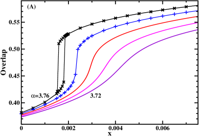
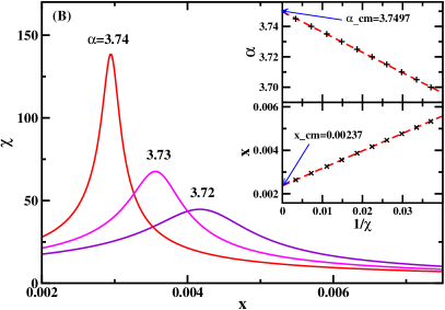
Figure 2: The mean overlap $\overline{q}(x)$ (A) and the overlap susceptibility $\chi(x)$ (B) at different constraint density values $\alpha$ for the random $3$-SAT problem. In (A) the value of $\alpha$ increases from $3.72$ to $3.76$ with step size $0.01$. The insets of (B) show that the peak value of $\chi$ diverges inverse linearly with $\alpha$ and $x$ as the critical point $(\alpha_{cm}=3.75,x_{cm}=0.0024)$ is approached (dashed lines are linear fittings).

Equations (6) and (7) can be solved by population dynamics methodMezard-Parisi-2001 . Some of the analytical results as obtained for the random $3$-SAT problem are shown in Fig. 2 (the results for $K\geq 4$ are qualitatively the same). When $\alpha<\alpha_{cm}=3.75$, the mean overlap $\overline{q}$ increases with the binding field $x$ smoothly, indicating that the solution space $\mathcal{S}$ of the random $3$-SAT problem is homogeneous. The overlap susceptibility $\chi(x)$ has a single peak, whose value is inverse proportional to $(\alpha_{cm}-\alpha)$ and diverges at $\alpha=\alpha_{cm}$ and $x=x_{cm}=0.0024$. The susceptibility $\chi(x)$ is again finite when $\alpha$ exceeds $\alpha_{cm}$, but the mean overlap $\overline{q}(x)$ changes discontinuously with $x$ at certain threshold value $x^{*}$. This first-order phase transition at $\alpha>\alpha_{cm}$ suggests that in the space $\mathcal{S}$ many solution communities (groups of similar solutions) are formed. For $x>x^{*}$ the partition function is predominantly contributed by intra-community solution-pairs (overlap favored), while for $x<x^{*}$ it is contributed mainly by inter-community solution-pairs (entropy favored). The different solution communities of $\mathcal{S}$ all belong to the same solution cluster ($s(q)$ is non-negative for any $q\in[q_{0},1]$) as long as $\alpha$ is less than $\alpha_{d}=3.87$Krzakala-etal-PNAS-2007 , but at $\alpha=\alpha_{d}$ they start to break up into different solution clusters ($s(q)$ is not defined for some intermediate $q$ valuesMora-Mezard-2006 ). At $\alpha=\alpha_{cm}$ the solution space $\mathcal{S}$ is in a critical state at which the boundaries between different solution communities disappear. This situation is qualitatively the same as the critical state of water at $647$K and $22.064$MPa, where the liquid and the gas phase are indistinguishable.

For the random $4$-SAT problem, we find that $\alpha_{cm}=8.4746$, which is consistent with the simulation results of Ref.Zhou-Ma-2009 . The value of $\alpha_{cm}$ is much below the clustering transition point $\alpha_{d}=9.38$Krzakala-etal-PNAS-2007 .

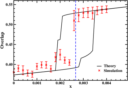
Figure 3: Mean overlap value of solutions with a reference solution $\vec{\sigma}^{*}$ for a single random $3$-SAT formula of $N=10^{5}$ vertices and constraint density $\alpha=3.85$. Solid lines are mean-field analytical result on this single formulaZhou-Ma-2009 , and the symbols with error bars are single-spin flips simulation results. Each sampled solution trajectory starts from $\vec{\sigma}^{*}$ and is equilibrated for at least $10^{7}$ Monte Carlo steps (each step corresponds to $N$ spin-flip attempts). More than $1000$ overlap values with $\vec{\sigma}^{*}$ are then sampled at time interval of $10^{4}$ Monte Carlo steps. The blue dashed line marks the equilibrium transition value of $x$.

The solution space heterogeneity can also be detected using single solutions as reference pointsZhou-Ma-2009 . Figure 3 shows the theoretical and simulation results on a random $3$-SAT formula with $N=10^{5}$ vertices and $M=3.85N$ constraints. The reference solution $\vec{\sigma}^{*}$ is uniformly randomly sampled from the solution space, and single-spin flips are used in the simulation to sample solutions $\vec{\sigma}$ with weight proportional to $\exp[Nxq(\vec{\sigma}^{*},\vec{\sigma})]$Zhou-Ma-2009 . The replica-symmetric cavity method predicts an equilibrium discontinuous change of the mean overlap value with solution $\vec{\sigma}^{*}$ at $x=x^{*}=0.00267$, which is confirmed by simulations. For $x>x^{*}$ most of the sampled solutions are in the same solution community of $\vec{\sigma}^{*}$, but for $x<x^{*}$ the sampled solutions are scattered in many different solution communities. Because of the high degree of structural heterogeneity, at $x<x^{*}$ it takes about $10^{7}$ Monte Carlo steps to travel from one solution community to another different community, making it very difficult to sample independent solutions.

When the solution space of the random $K$-SAT problem becomes heterogeneous at $\alpha\geq\alpha_{cm}(K)$, the replica-symmetric cavity theory, which leads to Eqs. (6)-(7), probably is not sufficient to describe its statistical properties. In a future publication we will report the result of the stability analysis on the replica-symmetric cavity equations, and present a mean-field study using the first-step replica-symmetry-breaking cavity theory.

IV Application to the random $K$-XORSAT problem

The $K$-XORSAT problem has wide-spread applications in low-density-parity-check codesMezard-Montanari-2009 and is also extremely studiedRicciTersenghi-Weigt-Zecchina-2001 ; Mezard-etal-2003 ; Cocco-etal-2003 ; Mora-Mezard-2006 . The constraint energy $E_{a}$ of this model is expressed in Eq. (1), where $J_{a}=\pm 1$ with equal probability. The solution space of a random $K$-XORSAT problem breaks into exponential solution clusters of equal size at a clustering transition point $\alpha=\alpha_{d}(K)$Mezard-etal-2003 ; Cocco-etal-2003 . We have applied the replica-symmetric cavity method to this problem and obtained the same qualitative results as for the random $K$-SAT problem, namely that before the ergodicity of the solution is broken, exponentially many solution communities start to form in the solution space as the constraint density reaches a critical value $\alpha_{cm}(K)$. At $\alpha=\alpha_{cm}(K)$ the solution space is in a critical state. For $K=3$ we find that $\alpha_{cm}(3)=0.6182$, which is much lower than the value of $\alpha_{d}(3)=0.818$RicciTersenghi-Weigt-Zecchina-2001 . For the random $4$-XORSAT problem, we find that $\alpha_{cm}(4)=0.504$, while $\alpha_{d}(4)=0.772$Mezard-etal-2003 .

The random $K$-XORSAT problem has a gauge symmetry that can be exploited to simply the mean-field calculationsMora-Mezard-2006 . Suppose $\vec{\sigma}^{1}$ is a solution, we can perform a gauge transformation $\sigma_{i}\rightarrow\tilde{\sigma}_{i}=\sigma_{i}\sigma_{i}^{1}$ to change the constraint energy Eq. (1) into $E_{a}=1-\prod_{i\in\partial a}\tilde{\sigma}_{i}$. All the coupling constants $J_{a}$ then become unity. The solution space structure of the random $K$-SAT problem looks the same from any a reference solution. We have used this nice property to calculate the total number of solutions that have a overlap value $q$ with a randomly chosen reference solution.

V Discussion

The main conclusion of this work is that, the solution space of a random constraint satisfaction problem has a transition to structural heterogeneity at a critical constraint density $\alpha_{cm}$, where many solution communities form. These solution communities serve as precursors for the splitting of the solution space into many solution clusters at a larger threshold value $\alpha_{d}$ of constraint density. This work brings a refined picture on how ergodicity of the solution space of a CSP finally breaks as the constraint density increases.

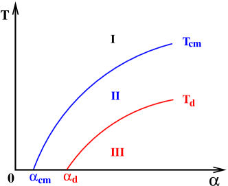
Figure 4: Schematic phase diagram for a constraint satisfaction problem, using temperature $T$ and constraint density $\alpha$ as control parameters. The configuration space is homogeneous and ergodic in region I. As the temperature $T$ decreases to $T_{cm}(\alpha)$, a homogeneity-breaking transition occurs, and the configuration space becomes non-homogeneous but still ergodic (region II). As $T$ further decreases to $T_{d}(\alpha)$, an ergodicity-breaking (clustering) transition occurs, and the configuration space breaks into many separated clusters (region III). At $T=0$, the ground-state configuration space is non-homogeneous at $\alpha\geq\alpha_{cm}$ and non-ergodic at $\alpha\geq\alpha_{d}$.

In spin-glass models with multi-spin interactions, the control parameter is often the temperature. The method presented here can also be used to study how the configuration spaces of these systems evolve with temperature. We suggest that similar heterogeneity transitions will occur before the clustering (or dynamical) transition. The following scenario is expected (see Fig. 4): at high temperatures the configuration space of a spin-glass or a lattice glass model system is in a homogeneous phase; as the temperature $T$ decreases to certain critical value $T_{cm}$, many communities of configurations form in the configuration space, and the configuration space is then in a heterogeneous but still ergodic phase; as $T$ decreases further to $T_{d}$, the different configuration communities separate into different Gibbs states, and the configuration space is no longer ergodic. The values of $T_{cm}$ for the random $K$-SAT problem and the random $K$-XORSAT problem as a function of the constraint density $\alpha$ will be calculated in a forthcoming publication. A related study was reported by Krzakala and Zdeborova recently on the the adiabatic evolution of single Gibbs states of a spin-glass system as a function of temperatureKrzakala-Zdeborova-2009 ; Zdeborova-Krzakala-2010 .

As the solution space of a CSP or the configuration space of a spin-glass or lattice glass system becomes heterogeneous and the configurations aggregate into many different communities, a stochastic search process based only on local rules (e.g., solution space random walkingZhou-2009 ) or a local dynamical process (e.g., single-particle heat-bath dynamics of a lattice glassDarst-Reichman-Biroli-2009 ) may get slowing down considerably and show heterogeneous behavior. The configuration space heterogeneity discussed in this paper probably is deeply connected to the phenomenon of spatial dynamical heterogeneity of glass-forming liquidsEdiger-2000 ; Cavagna-2009 . This research direction will be pursued in future work.

References

References

- (1) A. K. Hartmann and W. Weigt, Phase Transitions in Combinatorial Optimization Problems (Wiley-VCH, Weinheim, Germany, 2005).
- (2) M. Mézard and A. Montanari, Information, Physics, and Computation (Oxford Univ. Press, New York, USA, 2009).
- (3) R. Monasson and R. Zecchina, Phys. Rev. Lett. 76, 3881 (1996).
- (4) M. Mézard, G. Parisi, and R. Zecchina, Science 297, 812 (2002).
- (5) M. Mézard and G. Parisi, Eur. Phys. J. B 20, 217 (2001).
- (6) M. Mézard and G. Parisi, J. Stat. Phys. 111, 1 (2003).
- (7) G. Biroli and M. Mézard, Phys. Rev. Lett. 88, 025501 (2002).
- (8) R. K. Darst, D. R. Reichman, and G. Biroli, J. Chem. Phys. 132, 044510 (2010).
- (9) F. Krzakala, A. Montanari, F. Ricci-Tersenghi, G. Semerjian, and L. Zdeborova, Proc. Natl. Acad. Sci. USA 104, 10318 (2007).
- (10) A. Montanari and G. Semerjian, J. Stat. Phys. 124, 103 (2006).
- (11) M. Mézard and A. Montanari, J. Stat. Phys. 124, 1317 (2006).
- (12) F. Krzakala and J. Kurchan, Phys. Rev. E 76, 021122 (2007).
- (13) M. Alava, J. Ardelius, E. Aurell, P. Kaski, S. Krishnamurthy, P. Orponen, and S. Seitz, Proc. Natl. Acad. Sci. USA 105, 15253 (2008).
- (14) H. Zhou, Eur. Phys. J. B 73, 617 (2010).
- (15) H. Zhou and H. Ma, Phys. Rev. E 80, 066108 (2009).
- (16) M. D. Ediger, Annu. Rev. Phys. Chem. 51, 99 (2000).
- (17) S. C. Glotzer, J. Non-Cryst. Solids 274, 342 (2000).
- (18) A. Cavagna, Phys. Report 476, 51 (2009).
- (19) S. Mertens, M. Mézard, and R. Zecchina, Rand. Struct. Algorithms 28, 340 (2006).
- (20) T. Mora and M. Mézard, J. Stat. Mech.: Theor. Exp., P10007 (2006).
- (21) F. Ricci-Tersenghi, M. Weigt, and R. Zecchina, Phys. Rev. E 63, 026702 (2001).
- (22) M. Mézard, F. Ricci-Tersenghi, and R. Zecchina, J. Stat. Phys. 111, 505 (2003).
- (23) S. Cocco, O. Dubois, J. Mandler, and R. Monasson, Phys. Rev. Lett. 90, 047205 (2003).
- (24) F. Krzakala and L. Zdeborova, “Following Gibbs states adiabatically: The energy landscape of mean field glassy systems”, arXiv:0909.3820 (2009).
- (25) L. Zdeborova and F. Krzakala, Phys. Rev. B 81, 224205 (2010).