Matrix Inflation and the Landscape of its Potential

Abstract

Recently we introduced an inflationary setup in which the inflaton fields are matrix valued scalar fields with a generic quartic potential, M-flation. In this work we study the landscape of various inflationary models arising from M-flation. The landscape of the inflationary potential arises from the dynamics of concentric multiple branes in appropriate flux compactifications of string theory. After discussing the classical landscape of the theory we study the possibility of transition among various inflationary models appearing at different points on the landscape, mapping the quantum landscape of M-flation. As specific examples, we study some two-field inflationary models arising from this theory in the landscape.

Keywords : Matrix Theory, Inflation, Landscape.

I Introduction

The inflationary paradigm, the idea that the early Universe has undergone a nearly exponential expansion phase, has appeared as the leading candidate for explaining the recent cosmological observations data Komatsu:2008hk . The simplest and still successful model of inflation is a massive, free scalar field minimally coupled to the Einstein gravity. Nonetheless, motivated by various beyond the Standard Model particle physics or supergravity and string theory settings, many models of inflation have been constructed by introducing more non-trivial potentials for the scalar field and/or the addition of other scalar fields to the model.

The option of having a large number of scalar fields, instead of a handful of them, has been particularly motivated by string theory inspired models, where after fixing the moduli in compactifications they appear as light scalar fields subject to different potentials HenryTye:2006uv . A large number of (decoupled) scalars has the advantage that the contribution of each of them to the Hubble expansion parameter during inflation adds up, leading to a substantial number of e-folds, even if the potential for each field is not flat enough to sustain a successful period of inflation Liddle:1998jc . On the observational sides, a generic multiple field inflationary system predicts entropic and non-Gaussian perturbations which both are under intense observational constraints Komatsu:2008hk .

In Ashoorioon:2009wa , again motivated by string and D-branes settings, we introduced a model of inflation which has a large number of fields. In this model the inflaton fields were taken to be matrix valued objects and hence the model was dubbed as Matrix Inflation, or M-flation in short. The non-Abelian and non-commuting nature of matrices play a crucial role in M-flation construction.

We showed in Ashoorioon:2009wa that in a special corner of the rich “landscape” of the M-flation, one can reduce the theory to a standard chaotic inflationary model with at most a quartic potential. The matrix nature, however, now shows up in removing (or easing) the unnaturally small values of the couplings for these models. In this work we would like to analyze the landscape potential of M-flation in more detail. The landscape arises from the dynamics of coincident branes subject to appropriate fluxes in string theory compactification. At different points of this landscape we have inflationary models which are classically disconnected and the parameters at each point could be adjusted to achieve a period of slow-roll inflation with enough number of e-folds and acceptable spectral index. These different vacua, in principle, can tunnel to each other via quantum effects. If some fine-tunings of the couplings are tolerated, similar to the old inflation idea which should have terminated through first order phase transition Guth:1980zm , slow-roll inflation could end through bubble collision.

The paper is organized as follows. After reviewing the basic setup of M-flation in section II, we study the landscape of M-flation theories in section III. In section IV we analyze the landscape of the potential and hence inflationary models for a given Matrix inflation theory. Here we give a counting of various possible models (a counting on the landscape). This is basically a counting of number of $N\times N$ reducible representations of SU(2), which is much larger than $N^{2}$ for large $N$. We also discuss the tunneling between various vacua. As specific examples, we study some two-field inflationary models arising in our setup. In section V, we study numerically the physical predictions of these two-field models for CMB perturbations. The conclusions and discussions are provided in section VI. In Appendix A we present the cosmological perturbation theory for two field models in some details. In Appendix B, we consider the case where we have a positive energy metastable vacuum and find out the set of couplings where the first order phase transition from metastable vacuum to the true one is possible via quantum tunneling. As stated above, for a small window of parameters, nucleation rate is large enough to allow for a a first order phase transition via Coleman-De Luccia phase transition.

II M-flation, the Setup

As in Ashoorioon:2009wa we consider M-flation the inflationary model in which the inflaton fields are considered to be matrices and the inflationary potential is constructed from the matrices and their commutators. The action is

$$S=\int d^{4}x\sqrt{-g}\left(\frac{M_{P}^{2}}{2}R-\frac{1}{2}\sum_{i}\mbox{Tr}\left(\partial_{\mu}\Phi_{i}\partial^{\mu}\Phi_{i}\right)-V(\Phi_{i},[\Phi_{i},\Phi_{j}])\right)\,,$$ (II.1)

where the reduced Planck mass is $M_{P}^{-2}=8\pi G$ with $G$ being the Newton constant and the signature of the metric is $(-,+,+,+)$. Here the index $i$ counts the number of matrices and we take it to be $i=1,2,3$. The kinetic energy of $\Phi_{i}$ has the standard form and $\Phi_{i}$ are minimally coupled to gravity. To be specific, as in Ashoorioon:2009wa , we consider the following potential

$$V=\mbox{Tr}\left(-\frac{\lambda}{4}[\Phi_{i},\Phi_{j}][\Phi_{i},\Phi_{j}]+\frac{i\kappa}{3}\epsilon_{jkl}[\Phi_{k},\Phi_{l}]\Phi_{j}+\frac{m^{2}}{2}\Phi_{i}^{2}\right)\,,$$ (II.2)

which is quadratic in $\Phi_{i}$ or $[\Phi_{i},\Phi_{j}]$; (II.2) is the most general potential with this property. We choose the three parameters $\lambda,\ \kappa$ and $m^{2}$ to be non-negative.

The above action enjoys a global $U(N)$ symmetry under which $\Phi_{i}$ are in the adjoint. One may also consider the theory in which this $U(N)$ is gauged. The latter is done by replacing the partial derivatives of the scalars $\Phi_{i}$ by covariant derivatives, $D_{\mu}\Phi_{i}=\partial_{\mu}\Phi_{i}+ig[A_{\mu},\Phi_{i}]$, where $A_{\mu}$ is the gauge field, and by adding the Yang-Mills term for the gauge fields. For our purposes, during (slow-roll) inflation and as far as the classical dynamics of the scalars is involved, one may consistently set the gauge fields to zero, in which case the inflationary dynamics of the gauged and un-gauged models become identical. These two models, however, can have a different spectrum of linear perturbations about the inflationary background.

In Ashoorioon:2009wa we argued that this system, and in particular when the $U(N)$ symmetry is gauged, is strongly motivated from string theory where $\Phi_{i}$ represents the low energy dynamics of coincident branes in some specific flux compactifications Myers:1999ps . In this picture, $N$ coincident D3-branes extended along our Universe, subject to RR six-form field $C_{(6)}$, and through the Myers effect Myers:1999ps , can blow up into D5-branes, wrapping around a two-dimensional sphere in the extra three dimensions which are parameterized by matrix valued scalars $\Phi_{i}$. This two-sphere for finite $N$ is a fuzzy two-sphere and in the large $N$ limit it becomes a commutative round sphere. In Ashoorioon:2009wa we studied the case where $N\times N$ matrices exhibit a single fuzzy two-sphere. It is notable that in the large $N$ limit the sector of M-flation studied in Ashoorioon:2009wa , similar to Thomas:2007sj , Ward:2007gs and Berndsen:2009ww , is closely connected to the models of D5-branes wrapping two cycles of an internal (Calabi-Yau) space Becker:2007ui ; giant-inflaton . In these models the D5-branes are moving in a Klebanov-Strassler throat KS where the DBI effects become important. In this work, however, we would like to focus on the matrix effects. As we show below due to the matrix nature of the fields we have the possibility of multi-field inflationary models which does not exist in the analysis of Becker:2007ui ; giant-inflaton .

As we will show in this work, there is also the possibility that we have a large number of concentric fuzzy spheres of various radii, corresponding to a picture where we have more than one fuzzy sphere or wrapped D5-brane. Moreover, there is a distinct inflationary model associated with each of these multi-fuzzy spheres solutions: For the case of multi fuzzy spheres solution we obtain a multiple field inflationary model, where these scalar fields are classically decoupled from each other. These fields, similarly to the single field of Ashoorioon:2009wa , have the geometric interpretation of radii of the fuzzy spheres. To see this we analyze the equations of motion of the theory. Starting with an isotropic and homogenous FRW background

$$ds^{2}=-dt^{2}+a(t)^{2}d\vec{\bf x}^{\,2}\,,$$ (II.3)

the equation of motions are

$$H^{2}=\frac{1}{3M^{2}_{P}}\left(-\frac{1}{2}\mbox{Tr}\left(\partial_{\mu}\Phi_{i}\partial^{\mu}\Phi_{i}\right)+V(\Phi_{i},[\Phi_{i},\Phi_{j}])\right)$$ (II.4a)

$$\ddot{\Phi}_{l}+3H\dot{\Phi}_{l}+\lambda\left[\Phi_{j},\,[\Phi_{l},\Phi_{j}]\,\right]+i\,\kappa\,\epsilon_{ljk}[\Phi_{j},\Phi_{k}]+m^{2}\Phi_{l}=0\,,$$ (II.4b)

$$\dot{H}=-\frac{1}{2M^{2}_{P}}\ \sum_{i}\mbox{Tr}\partial_{\mu}\Phi_{i}\partial^{\mu}\Phi_{i}\ ,$$ (II.4c)

where $H=\dot{a}/a$ is the Hubble expansion rate.

It is straightforward to check that the above equations of motion can be solved with $\Phi_{i}$ in the matrix form

$$\Phi_{i}=\sum_{\alpha}\hat{\phi}_{\alpha}J_{i}^{\alpha}\quad,\quad i=1,2,3$$ (II.5)

where $J_{i}^{\alpha}$ are $N_{\alpha}\times N_{\alpha}$ matrices satisfying the $SU(2)$ algebra

$$[J_{i}^{\alpha},J_{j}^{\beta}]=i\epsilon_{ijk}\delta^{\alpha\beta}\ J_{k}^{\alpha}\ ,\qquad Tr(J_{i}^{\alpha}J_{j}^{\beta})=\frac{1}{4}N_{\alpha}(N^{2}_{\alpha}-1)\delta_{ij}\delta^{\alpha\beta}\ .$$ (II.6)

Here $N_{\alpha}$ are arbitrary non-negative integers subject to the condition $\sum_{\alpha}N_{\alpha}=N$. That is, $\sum_{\alpha}J_{i}^{\alpha}$ form reducible $N\times N$ representation of $SU(2)$. In the above, the value of $\alpha$ specifies the number of irreducible $SU(2)$ blocks in the generic $N\times N$ matrix. Therefore, the range of $\alpha$ can vary from one, corresponding to a single irreducible representation which was discussed in some details in Ashoorioon:2009wa , to $N$, where basically we have the solution $\Phi_{i}=0$.

In fact, one can show that (II.5) is the most general solution to (II.4b). Moreover, sum of two solutions of the form (II.5) is not a solution to (II.4b). With the above decomposition one finds that the equations for $\hat{\phi}_{\alpha}$ decouple and one may analyze them separately. It is then convenient to rewrite the action in terms of $\hat{\phi}_{\alpha}$, rather than the matrices $\Phi_{i}$. Doing so, and after rescaling

$$\hat{\phi}_{\alpha}=\left[\frac{1}{4}N_{\alpha}(N^{2}_{\alpha}-1)\right]^{-1/2}\phi_{\alpha}\ ,$$ (II.7)

we obtain a multi-field canonically normalized action for the scalars $\phi_{\alpha}$ with the potential

$$V(\phi_{\alpha})=\sum_{\alpha}\ \frac{\lambda_{\alpha}}{4}\phi_{\alpha}^{4}-\frac{2\kappa_{\alpha}}{3}\phi_{\alpha}^{3}+\frac{m^{2}}{2}\phi_{\alpha}^{2}$$ (II.8)

where

$$\lambda_{\alpha}=\frac{8\lambda}{N_{\alpha}(N_{\alpha}^{2}-1)}\ ,\qquad\kappa_{\alpha}=\frac{2\,\kappa}{\sqrt{N_{\alpha}(N_{\alpha}^{2}-1)}}.$$ (II.9)

As we see the fields $\phi_{\alpha}$ are decoupled from each other, which is in fact the result (or advantage) of using the $SU(2)$ basis we have introduced. Note that although in the potential (II.8) there is no interaction between $\phi_{\alpha}$, they all couple to gravity and contribute to $H$. Therefore, their dynamics are coupled through gravity.

From now on we call each reducible solution which minimizes the potential a “vacuum” solution. In Ashoorioon:2009wa we analyzed the irreducible vacuum, where we studied the $N_{\alpha}=N$ case in which $\alpha=1$ and as such this vacuum may also be called the “single block vacuum” or the “single giant vacuum” (in a reference to the blown-up D3 branes picture). Similarly, when $\alpha$ ranges from one to $n$ we have an $n$-block vacuum or $n$-giant vacuum.

III The Landscape of M-flation theories

There are four parameters in the original M-flation action, $\lambda,\ \kappa,\ m^{2}$ and the size of matrices $N$. As discussed above, the classical solutions of the theory are described by the set of parameters $(\lambda_{\alpha},\kappa_{\alpha},m^{2})$ and the set of $N_{\alpha}$ which are subject to $\sum_{\alpha=1}^{n}N_{\alpha}=N$. Depending on parameters $(\lambda_{\alpha},\kappa_{\alpha},m^{2})$ one obtains potentials of different forms. Since the potential (II.8) is the sum of potentials which only depend on a single field $\phi_{\alpha}$, we may analyze each of them independently. The latter is basically the shape of the potential about the single-block vacuum which is studied first. We then analyze the multi-field case.

III.1 Analysis of the potential around the single-block (irreducible) vacuum

As a starter, we briefly review, summarize and expand on the results of Ashoorioon:2009wa , where Matrix Inflation theory is effectively reduced to a single scalar field theory corresponding to $\alpha=1$ in Eq. (II.5). For that purpose we assume the $N\times N$ matrix part of $\Phi_{i}$ to be proportional to the generators of $SU(2)$ algebra in its $N\times N$ irreducible representation. Upon the rescaling

$$\hat{\phi}=\left[\frac{1}{4}N(N^{2}-1)\right]^{-1/2}\phi\ ,$$ (III.1)

the action reduces to a canonically normalized scalar field theory coupled to Einstein gravity with the potential

$$V_{S}(\phi)=\frac{\lambda_{\phi}}{4}\phi^{4}-\frac{2\kappa_{\phi}}{3}\phi^{3}+\frac{m^{2}}{2}\phi^{2}$$ (III.2)

where

$$\lambda_{\phi}=\frac{8\lambda}{N(N^{2}-1)}\ ,\qquad\kappa_{\phi}=\frac{2\,\kappa}{\sqrt{N(N^{2}-1)}}\,.$$ (III.3)

Depending on the value of the ratio $m^{2}\lambda_{\phi}/\kappa^{2}_{\phi}=2m^{2}\lambda/\kappa$ we may have five different cases. Note the remarkable property that this ratio is $N$-independent. In Fig. 1 we have plotted the different shapes of the potential. Since in the string theory setup, $\hat{\phi}_{\alpha}$ represents the radius of each fuzzy sphere, we take $\phi_{\alpha}$ to be positive.

(I)           (II) (III)           (IV) (V)

Figure 1: Different possible shapes of the single block potential Eq. (III.2).

• Case I)  $\kappa^{2}<2m^{2}\lambda$.

  In this case the potential has only a single minimum at $\phi=0$ for which the potential vanishes. All the $\kappa=0$ cases, including $\lambda\phi^{4}$ and $m^{2}\phi^{2}$ chaotic inflation potentials are in this class.

  For the rest of cases $\kappa^{2}\geq 2m^{2}\lambda$ and hence one may use the parameterization

  $$\sin^{2}\Theta\equiv\frac{2m^{2}\lambda}{\kappa^{2}}\ \qquad\Theta\in[0,\pi/2].$$ (III.4)

• Case II)  $\Theta=\frac{\pi}{2}$.

  In this case the potential has an inflection point which happens at $\phi_{0}=\frac{\kappa_{\phi}}{\lambda_{\phi}}$. The value of potential at the inflection point is

  $$V_{S}^{0}=\frac{\kappa^{4}}{384\lambda^{3}}\ N(N^{2}-1)\ .$$

  As discussed in Ashoorioon:2009wa the inflationary model based on this case has a small red spectral index and is on the verge of being ruled out.

• Case III)  $\sin^{-1}(\frac{8}{9})<\Theta<\frac{\pi}{2}$.

  In this case the potential besides the zero energy minimum at $\phi=0$ has also a minimum at

  $$\phi_{0}=\frac{\kappa_{\phi}}{\lambda_{\phi}}(1+\cos\Theta)\ ,$$ (III.5)

  and the energy

  $$V_{S}^{0}=\frac{\kappa^{4}}{384\lambda^{3}}\ N(N^{2}-1)\ F(\Theta)\ ,$$ (III.6)

  where

  $$F(\Theta)=(1-3\cos\Theta)(1+\cos\Theta)^{3}.$$

  In this case $V_{S}^{0}>0$. If the inflationary dynamics happens around the $\phi_{0}$ minimum such that the end point of the slow-roll inflationary phase is at $\phi_{0}$, then the situation is like old inflation and we are back to the “graceful exit” problem. In Appendix B, we have determined the set of parameters for which nucleation rate via Coleman-De Luccia Coleman:1980aw quantum tunneling is substantial to cause a first order phase transition at $\phi_{0}$. We have also shown that it is not possible to tunnel from the false vacuum to the true one by Hawking-Moss Hawking:1981fz phase transition, if one demands the COBE normalization for density perturbations in the subsequent slow-roll phase.

• Case IV)  $\Theta=\sin^{-1}(\frac{8}{9})$.

  In this case $\phi_{0}=4\kappa_{\phi}/3\lambda_{\phi}$ and $F(\Theta)=0$ so the energy of the potential at the minimum vanishes. In Ashoorioon:2009wa this case was called the “symmetry breaking” potential. This case does not suffer from the secondary old inflation phase and hence is a preferred case for building an inflationary scenario. Moreover, the potential in this case has the remarkable property that it could be obtained from a cubic superpotential and hence the model can be embedded in a supersymmetric theory. This latter gives us a better control over the running of the parameters and the Coleman-Weinberg corrections. In string theory set up, the minimum at $\phi_{0}$ corresponds to the configuration when $N$ coincident D3-branes blow up into the supersymmetric configuration of a giant fuzzy sphere with radius determined by $\phi_{0}$. The other vacuum, $\phi=0$, corresponds to the configuration of commuting matrices with a shrinking size sphere.

• Case V)  $0\leq\Theta<\sin^{-1}(\frac{8}{9})$.

  In this case $F(\Theta)<0$ and the global minimum is at $\phi_{0}$ with an AdS vacuum. The $m^{2}=0$ case, which is the case usually studied in the D-brane setting in string theory (see e.g. Myers:1999ps ; Wadia ; giant-inflaton ), falls in this class. It is possible to have slow-roll inflation around the minimum $\phi=0$. The minimum at $\phi_{0}$ is an AdS type and is not suitable as an end point for inflation. As discussed in Coleman:1980aw the gravitational effects makes the $\phi=0$ vacuum stable against tunneling to true vacuum at $\phi_{0}$.

In the specific examples of two-field models studied in the following section, we restrict our analysis mainly to the cases I) and IV) above.

III.2 Analysis of the potential for $n$-block vacua

We now consider a general $n$-block vacuum, corresponding to the $n$-field inflationary potential (II.8) with (II.9). In this case the equation of motion for the fields $\phi_{\alpha}$ (when gravity is turned off) are essentially decoupled from each other. Nonetheless, all of them are coupled to the background metric and give contributions to the Hubble parameter and hence the field $\phi_{\alpha}$ will feel the effects of the other fields through the evolution of the background metric. The equations of motion for the $n$-field theory are

$$H^{2} =\frac{1}{3M_{P}^{2}}\sum_{\alpha=1}^{n}\left(\frac{1}{2}\dot{\phi}_{\alpha}^{2}+V_{\alpha}(\phi_{\alpha})\right)$$ (III.7a)

$$\ddot{\phi}_{\alpha}+3H\dot{\phi}_{\alpha}+\partial_{{\phi_{\alpha}}}V_{\alpha}=0\ ,$$ (III.7b)

where $V_{\alpha}(\phi_{\alpha})$ is given by Eq. (II.8).

Noting that the angle $\Theta$ given by Eq. (III.4) is independent of $N_{\alpha}$, the form of the potentials $V_{\alpha}$ (in the sense that which of the five cases of previous subsection they fall into) is independent of $\alpha$ and hence for a generic $n$-block vacuum we still have the same five cases discussed above. The value of the potential at the minimum and at which $\phi_{\alpha}$ the minimum happens, however, depend on $N_{\alpha}$.

In summary, irrespective of which set of $\{N_{\alpha}\}$ is chosen, the generic shape of the inflationary potentials falls into one of the five cases discussed above and is completely specified by the dimensionless ratio $\kappa^{2}/(m^{2}\lambda)$.

IV Landscape of $n$-block Matrix Inflation

In the previous section we analyzed different possibilities for the generic behavior of the inflationary potential depending on how the original parameters of M-flation is chosen. In this section we study the landscape of various inflationary models arising from inflation assuming a given set of parameters $(\lambda,\kappa,m^{2})$ and $N$.

IV.1 Counting the number of vacua in the landscape

As the first piece of information on the rich landscape of the potentials, which all are in the generic form of (II.8) with (II.9), we present a counting of these vacua. The case of single block, $n=1$, was studied in III.1 and depending on the ratio $m^{2}\lambda/\kappa^{2}$ we may have either of the five distinct cases discussed earlier. Next, we may consider the double block vacuum, which leads to a two-field inflationary potential. In this case, the number of possibilities is the same as the ways one can partition $N$ into two positive integers. Denoting the size of two blocks by $N_{1}$ and $N_{2}$, $N_{1}+N_{2}=N$, with $N_{1}\geq\ N_{2}\geq 1$, one has $[\frac{1}{2}N]$ possible solutions, where $[x]$ is the integer part of $x$. (Note that exchanging $N_{1}$ and $N_{2}$ does not lead to a different theory.) In other words, there are $[\frac{1}{2}N]$ possible two-field models coming out of M-flation.

In a similar way one may count ${\cal N}_{n}(N)$, the number of independent $n$-field inflationary models arising from M-flation (which is the same as the number of vacua or the minima of the potential). ${\cal N}_{n}(N)$ is the number of ways an integer $N$ can be partitioned into $n$ positive integers $N_{i}$ such that $\sum_{i=1}^{n}N_{i}=N$, $1\leq N_{i}\leq N_{i+1}$. One can show that

$${\cal N}_{n}(N)=\sum_{k=1}^{[\frac{N}{n}]}{\cal N}_{n-1}(N+n-1-nk),\qquad{\cal N}_{1}=1,$$ (IV.1)

for $n\leq\frac{N}{2}$ and

$${\cal N}_{n}(N)={\cal N}_{N-n}(2(N-n))\ ,$$ (IV.2)

for $n\geq\frac{N}{2}$. From the above recursion relations one can compute ${\cal N}_{n}(N)$. For example, for $n=2$, ${\cal N}_{2}=[\frac{N}{2}]$ and for $n=N$, ${\cal N}_{N}=1$. For large $N$, and when $n\ll N$ one can show that ${\cal N}_{n}(N)\sim\frac{1}{n!}(N-1)\cdots(N-n+1)\sim\frac{1}{n!}N^{n-1}$. The number of points (theories) in the landscape of the possible theories, for a given set of parameters $(\lambda,\kappa,m^{2})$ and $N$ is

$${\cal N}_{total}=\sum_{n=1}^{N}\ {\cal N}_{n}\sim\frac{2^{N}}{N}\ ,$$ (IV.3)

for large $N$.

It is worth noting that around each minimum point in this landscape we have an n-field model specified with $\{N_{\alpha}\}$, where $\alpha=1,2,\cdots,n$. Around each point there are $3N^{2}-n$ fields where $N=\sum_{\alpha=1}^{\alpha=n}N_{\alpha}$, that are not classically excited. These fields, which are not classically coupled to the $n$ inflationary fields, can appear through quantum excitations of the fields, leading to $3N^{2}-n$ isocurvature fields. In summary, among the cosmic perturbations around the specific $n$-block vacuum, we have one usual curvature (adiabatic) mode, $n-1$ entropy modes and $3N^{2}-n$ isocurvature modes.

IV.2 Transition between multi-field scenarios

As discussed, if we start with the initial condition that the matrix valued fields $\Phi_{i}$ and their time derivative $\dot{\Phi}_{i}$ are given in terms of the generic $SU(2)$ (reducible) representation, the dynamics of M-flation is such that they always remain in the same sector. In this sense the classical (inflationary) dynamics around the “multi giant vacua” decouple from each other and one may build an inflationary model around either of these. If we start with a field which is initially in the sector specified by a given set of $N_{\alpha}$, then $N_{\alpha}$ remains a conserved quantity by the classical trajectory of the system. In general various fields in the same sector specified by a set of $N_{\alpha}$ can mix with each other. That is, in general the inflationary trajectory in the space of $\phi_{\alpha}$ is curved. We will discuss the details of the inflationary dynamics for the special two-field case in the next section.

This “classical” decoupling can, however, break due to quantum effects and one can find various quantum paths connecting vacua with different sets of $N_{\alpha}$. To see this let us suppose that the ratio $m^{2}\lambda/\kappa^{2}$ takes a generic value and for the ease of the analysis consider the epoch the inflationary dynamics has ended and the fields are settled in the minimum of their potential. Let us study the tunneling between vacua corresponding to two $SU(2)$ reducible representations specified by sets of $N^{(1)}_{\alpha}$ and $N^{(2)}_{\alpha}$ which will respectively be denoted by $J_{i}^{(1)}$ and $J_{i}^{(2)}$. One such path between the two vacua is

$$\Phi_{i}=\phi(t)J_{i}^{(1)}+(1-\phi(t))J_{i}^{(2)}\ ,\qquad\phi(t=0)=1,\ \phi(t=t_{0})=0.$$ (IV.4)

One may then evaluate and minimize the action for the above path and use the WKB approximation to compute the transition amplitude by exponentiating the value of the Euclidean action. (We comment that there are other paths over which the action is smaller compared to the one evaluated for the above path. In such cases these paths would dominate the tunneling.)

The transition may happen from a local minimum with higher (or equal) energy to a local minimum with lower (or the same) energy. To be specific let us compare the irreducible (single-giant) vacuum with a generic $n$-giant vacuum. Depending on the value of the ratio $m^{2}\lambda/\kappa^{2}$ the single or $n$-giant vacua could have a higher energy. It is readily seen that

$$V_{S}^{0}-V_{n-\rm{field}}^{0}=\frac{N^{3}-\sum_{\alpha}N_{\alpha}^{3}}{N(N^{2}-1)}V_{S}^{0}\ ,\qquad\sum_{\alpha}N_{\alpha}=N\ .$$ (IV.5)

and hence $V_{S}^{0}-V_{n-\rm{field}}^{0}$ has the same sign as $V_{S}^{0}$. Explicitly, for the case III the $n$-giant vacuum is more stable and the single giant vacuum can decay (tunnel) into the multi-field vacua, as well as tunneling into its own $\phi=0$ vacuum. For the case V, we have an opposite situation and the single giant vacuum is the most stable one and the multi-giant vacua can tunnel into the single giant one. Such an analysis has been carried out in Wadia . The symmetry breaking case, case IV, is special in the sense that $V_{S}^{0}=0$ and hence all the vacua have the same energy. The calculation of the transition amplitude for this case has been carried out in some detail in DSV . In the analysis there it has been shown that the path which minimizes the action is not of the form (IV.4). In DSV it is shown that the height of the potential between the two vacua grows like $N^{2}$ (for large $N$), unlike the $N^{3}$ expected from a path like (IV.4).

One may also provide a picture for the above tunneling in terms of transition between a multi-giants configuration to a single giant one. Let us consider the specific case of transition between two and single giant configurations. As was discussed the above reducible solution with two blocks (in the large $N_{1},N_{2}$ limit) has the interpretation of concentric spherical D-branes whose radii, $N_{1}\hat{\phi}_{1}/2$ and $N_{2}\hat{\phi}_{2}/2$ are changing in time. Analysis of DSV suggests a transition between the two is dominated by the path which is mediated through nucleation of a throat between the two giants, which eventually dissolves them into a single giant (or vice versa), as depicted in Fig. 2. These throats are basically the virtual open string loops which are stretched between the giants (branes).

Figure 2: Two possible paths for quantum tunneling between two block and single block vacua. The top figure shows a paths in which the spherical symmetry of the giants are preserved along the path. The figure below shows a path in which the transition happens through nucleation of a throat between the two giants, through which the inner giant is eventually dissolved into the outer one. Both of these paths are coming from quantum fluctuations of the two initial giants and can be understood as specific modes of open strings stretched between the two giants. Analysis of DSV shows that the path depicted in the lower figure dominates the transition.

Moreover, there is also a non-zero tunneling amplitude from the non-trivial “giant” graviton vacuum to the vacuum at $\phi=0$. For the case of supersymmetric theories some of these paths may be forbidden due to supersymmetry.

V Two-Block Matrix Inflation

We have discussed that dynamics in a sector with a given set of $N_{\alpha},\ \alpha=1,2\ ,\cdots,n$ can decouple from the rest of the theory if we initially start in that sector. Although the inflationary potential in this sector contains $n$ decoupled scalars, they are in general coupled to each other through gravitational interactions, leading to $n$-field inflationary models. In this section we analyze in some details the simplest of such models, i.e. the two-field case for which the field $\Phi_{i}$ can be expanded as

$$\Phi_{i}=\hat{\phi}(t)J^{(1)}_{i}+\hat{\chi}(t)J^{(2)}_{i}\,,$$ (V.1)

where $J^{(1)}_{i}$ and $J^{(2)}_{i}$ are respectively $N_{1}$ and $N_{2}$-dimensional ($N_{1}+N_{2}=N$) irreducible representations of $SU(2)$ algebra. In the string theory setup studied in Ashoorioon:2009wa , the fields $\hat{\phi}$ and $\hat{\chi}$ indicate the radius of the giant spheres to which the stacks of coincident branes are blown up. Since $\Phi_{i}$, $J^{(1)}_{i}$ and $J^{(2)}_{i}$ are Hermitian, we conclude that $\hat{\phi}$ and $\hat{\chi}$ are real scalar fields.

After rescaling the $\hat{\phi}_{\alpha}$, $\lambda$ and $\kappa$ as in (II.7) and (II.9) we obtain the effective two field potential

$$V_{D}(\phi,\chi)=\frac{\lambda_{\phi}}{4}\phi^{4}+\frac{\lambda_{\chi}}{4}\chi^{4}-\frac{2\kappa_{\phi}}{3}\phi^{3}-\frac{2\kappa_{\chi}}{3}\chi^{3}+\frac{m^{2}}{2}\left(\phi^{2}+\chi^{2}\right)\ .$$ (V.2)

The effective couplings $\lambda_{\phi},\lambda_{\chi},\kappa_{\phi}$ and $\kappa_{\chi}$ are given by

$$\lambda_{\phi}=\frac{8\lambda}{N_{1}(N_{1}^{2}-1)}\ ,\qquad\kappa_{\phi}=\frac{2\,\kappa}{\sqrt{N_{1}(N_{1}^{2}-1)}}$$ (V.3)

with a similar expressions for $\lambda_{\chi},\kappa_{\chi}$ with $N_{1}$ replaced by $N_{2}$.

With the initial condition of solutions given by Eq. (V.1), our system is basically reduced into a two-field inflationary system of $\phi$ and $\chi$. The background equations of motion are

$$H^{2}=\frac{1}{3M_{P}^{2}}\left[\frac{1}{2}\dot{\phi}^{2}+\frac{1}{2}\dot{\chi}^{2}+V_{D}(\phi,\chi)\right]$$

$$\ddot{\phi}+3H\dot{\phi}+\partial_{\phi}V_{D}=0\quad,\quad\ddot{\chi}+3H\dot{\chi}+\partial_{\chi}V_{D}=0\,.$$ (V.4)

Since $m^{2}\lambda_{\phi}/\kappa^{2}_{\phi}=m^{2}\lambda_{\chi}/\kappa^{2}_{\chi}$, depending on the value of this ratio, the potential $V_{D}$ can be classified into exactly the same five cases studied in subsection (III.1) and hence we do not repeat them here. Below we study some inflationary backgrounds constructed from $V_{D}(\phi,\chi)$. For some details of the treatment of the cosmological perturbation theory for two-field models see Appendix A.

For general initial conditions, the inflationary trajectory is curved in the $\phi$-$\chi$ plane. The general result of such an effect will be a nonzero correlation between the adiabatic and the entropy perturbations. The magnitude of the effect, however, depends on the values of the couplings and the initial conditions. We consider the following cases, which shows to what extent the results are initial condition-dependent.

V.1 Quartic Potential

Suppose $\kappa=m=0$. The background inflationary potential

$$V=\frac{\lambda_{\phi}}{4}\phi^{4}+\frac{\lambda_{\chi}}{4}\chi^{4}\,,$$ (V.5)

has the form of case I.

Considering number of e-folds, $N_{e}$, as the clock $Hdt=-dN_{e}$, in the slow-roll limit one can check that

$$\phi\simeq\sqrt{8N_{e}}M_{P}\sin\alpha\quad,\quad\ \chi\simeq\sqrt{8N_{e}}M_{P}\cos\alpha\,,$$ (V.6)

where $\alpha$ is an angle. Furthermore, the trajectory in $(\phi,\chi)$ space or $(N_{e},\alpha)$ space is

$$\phi^{-2}=R^{2}\chi^{-2}+C\quad,\quad N_{e}=\frac{8M_{P}^{2}}{C}\left(\sin^{-2}\alpha-{R^{2}}\cos^{-2}\alpha\right)$$ (V.7)

where $C$ is a constant of integration and $R$ is the ratio of the couplings

$$R^{2}\equiv\frac{\lambda_{\phi}}{\lambda_{\chi}}=\frac{N_{2}(N_{2}^{2}-1)}{N_{1}(N_{1}^{2}-1)}\,.$$ (V.8)

The analysis is similar to Polarski:1992dq ; Polarski:1994rz and Langlois:1999dw .

For the numerical study, we first consider the case where the quartic coupling of $\chi$ and $\psi$ are of the same order. In this case the trajectory is slightly curved, if the initial conditions of none of the two fields are set to zero. For definiteness, we assume that

$$\lambda_{\phi}=2.05\times 10^{-13}\quad,\quad\lambda_{\chi}=5\times 10^{-13}$$

$$\phi_{i}=22.437~{}M_{P}\quad,\quad\chi_{i}=8~{}M_{P},$$ (V.9)

where the initial value of fields, $\phi_{i}$ and $\chi_{i}$, are given $71$ e-folds before the end of inflation. Choosing the natural bare value of $\lambda\sim 1$, from Eq. (V.3), the above values for the effective quartic couplings correspond to the following values for the dimensions of the blocks:

$$N_{1}\simeq 34000\quad,\quad N_{2}\simeq 25000\,.$$ (V.10)

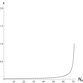
Figure 3: Left graph shows the trajectory for two quartic potentials with comparable quartic couplings. Right graph shows the slow-roll parameter, $\epsilon$, as a function of number of e-folds.

The trajectory in $\phi$-$\chi$ plane is given in left graph of Fig.3. It contains both the analytical curve Eq. (V.7) and the exact numerical results which indicate that the slow-roll approximation is very well valid until the end of inflation. We have also graphed the first slow-roll parameter

$$\epsilon=\frac{M_{P}^{2}}{2}\left(\frac{V_{\sigma}}{V}\right)^{2}\,,$$ (V.11)

in terms of number of e-folds in the right graph. As one can see, $\epsilon$ changes smoothly up to the end of inflation. The value of quartic couplings are chosen such that the amplitude of density perturbations for the mode that exit $60$ e-folds before the end of inflation, $k_{60}$, is COBE normalized, i.e. $P_{\mathcal{R}}(k_{60})=2.4\times 10^{-9}$. The scalar spectral index at such scales is $n_{\mathcal{R}}(k_{60})\simeq 0.947$, which is slightly smaller than single $\lambda\phi^{4}$ model, but still within the $2\sigma$ level of WMAP results.

The amplitude of correlated entropy mode is $4.4\times 10^{-17}$ at the current horizon scale and has a spectral index of $\simeq 0.9837$. The correlation between curvature and entropy perturbations, $\mathcal{C}$, is $0.228$ at such scales which shows that curvature perturbations at these scales are partially generated through the transformation of entropy perturbations to curvature ones. The amplitude of tensor perturbation is $P_{T}(k_{60})\simeq 6.33\times 10^{-10}$, corresponding to $r\simeq 0.26$ which is on the verge of being ruled out by the future experiments. The tensor spectral index, $n_{T}$, is $\simeq-0.036$. One should note that the consistency relation between tensor and scalar spectra for single field inflation, $r=-8n_{T}$, changes to $r=-8n_{T}(1-\mathcal{C}^{2})$ in such two-field models Wands:2002bn , which is confirmed by our numerics. In this sense the two-field $\lambda\phi^{4}$ theory is subject to a lower tensor-to-scalar ratio $r$ than the single field case. Hence it may fall in the region of $n_{s}-r$ plane which is allowed by WMAP5. (c.f. Ashoorioon:2005ep for the violation of consistency relation in the context of trans-Planckian physics).

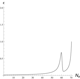
Figure 4: Left graph shows the trajectory for two quartic potentials with hierarchy in quartic couplings. There is a transient non-slow-roll phase in the evolution of the fields. The solid and dashed curved, respectively, denote the analytic and numerical results. Right graph shows the slow-roll parameter, $\epsilon$, as a function of number of e-folds.

In the other example that we will consider, there will be a transient period of fast-roll evolution. To realize such a scenario there should be a hierarchy between $\lambda_{\phi}$ and $\lambda_{\chi}$. Inflation will not stop, nonetheless $\epsilon$ approaches close to unity for few e-folds. Before this transient period, inflation is basically driven by one of the fields and after that by the other. In $\lambda\phi^{4}$ model, the spectral index depends on the number of e-folds, $N_{e}$, via the relation, $n_{\mathcal{R}}=1-3/N_{e}$. Thus if the first phase lasts less than $50$ e-folds, the scalar spectral index easily falls outside the $2\sigma$ limit of WMAP5 central value for the spectral index. Therefore double inflation models like Polarski:1992dq , consistent with predictions in the CMB regime, are difficult to be produced with two quartic potentials. Nonetheless, we investigate this possibility that such a non-slow-roll phase occurs toward the end of inflation. In the following example we have tuned the parameters such that the non-slow-roll phase occurs in the last $10$ e-folds of inflation:

$$\lambda_{\phi}=2.05\times 10^{-13}\quad,\quad\lambda_{\chi}=5\times 10^{-16}$$

$$\phi_{i}=21.8~{}M_{P}\quad,\quad\chi_{i}=9.1~{}M_{P}\,.$$ (V.12)

Initial values for the fields are given $70.34$ e-folds before the end of inflation. The exact numerical trajectory is shown in the left graph of Fig. 4 by the solid curve, whereas the analytic trajectory, given by formula (V.7), is shown by the dashed one. The mismatch between the two curves is a result of slow-roll violation at the end of inflation. We have also included the behavior of the slow-roll parameter, $\epsilon$, vs. $N_{e}$ which shows that for few e-folds $\epsilon$ increases considerably. Tuning the values of quartic couplings such that the amplitude of density perturbations matches the COBE normalization, one obtains $n_{\mathcal{R}}(k_{60})\simeq 0.941$. The amplitude of correlated entropy perturbations are $1.79\times 10^{-20}$ whose spectral index is $\simeq 0.958$. The relative cross correlation between curvature and entropy perturbations is $0.411$ which has a blue spectral index $\simeq 8.4\times 10^{-3}$. The amplitude of gravity waves at Hubble scale is $\simeq 6.42\times 10^{-10}$, i.e. $r\simeq 0.328$, which shows that this model is completely excluded by the observations.

Figure 5: The graphs show the trajectory for two symmetry-breaking cases considered in the manuscript.

V.2 Symmetry Breaking

The next example we study corresponds to the symmetry breaking potential where

$$V=\frac{\lambda_{\phi}}{4}\phi^{2}(\phi-\mu_{\phi})^{2}+\frac{\lambda_{\chi}}{4}\chi^{2}(\phi-\mu_{\chi})^{2}\,.$$ (V.13)

Using the equations of motions for $\phi$ and $\chi$ combined with Friedmann equation one can show that the curved inflationary trajectory in $\phi-\chi$ field space is

$$\phi(\phi-\mu_{\phi})+\chi(\chi-\mu_{\chi})-\frac{\mu_{\phi}^{2}}{2}\ln(2\phi-\mu_{\phi})-\frac{\mu_{\chi}^{2}}{2}\ln(2\chi-\mu_{\chi})=8M_{P}^{2}\,N_{e}\,.$$ (V.14)

We consider the following values for the couplings:

$$\lambda_{\phi}=2\times 10^{-15},\quad\mu_{\phi}=196.168M_{P},\quad\mu_{\chi}=36M_{P},\quad\lambda_{\chi}=\lambda_{\phi}{\left(\frac{\mu_{\phi}}{\mu_{\chi}}\right)}^{2}$$

$$\phi_{i}=209.439~{}M_{P}\quad,\quad\chi_{i}=26.678~{}M_{P}$$ (V.15)

The trajectory in the $\phi-\chi$ plane is given in the left graph of Fig. 5 . The theoretical curve Eq. (V.14) and the curve obtained from the full numerical analysis coincide with each other which indicates that the slow-roll approximation is very well valid up to the end of inflation. For this model, $n_{\mathcal{R}}\simeq 0.963$, which is compatible with WMAP 5 years results. The amplitude and spectral index of correlated entropy mode are respectively $1.4\times 10^{-13}$ and $0.978$ at horizon scales. The amplitude of correlation factor between curvature and entropy mode is $\mathcal{C}\simeq 0.602$. For gravity waves, the amplitude and spectral index are respectively, $P_{T}(k_{60})=2.618\times 10^{-10}$, i.e. $r\simeq 0.107$, and $n_{T}\simeq-0.041$.

Another interesting case that has a nice geometric interpretation is when $N_{1}=N_{2}$ and $\phi_{i}>\chi_{i}$. In the string theory picture, this corresponds to two stacks of D3-branes where in the background of RR six form, $C_{(6)}$, two of their perpendicular dimensions are blown-up to two concentric spheres, one of which has a radius smaller than $\mu$ and the other one bigger than $\mu$. The bigger one shrinks and the smaller one expands. These two spheres collide when their radii reaches $\mu$ and pass through each other. This incident happens well after the end of inflation and during preheating and may have interesting consequences. One set of parameters for which, the above scenario is realized is given below:

$$\lambda_{\phi}=\lambda_{\chi}=6\times 10^{-14},\quad\mu_{\phi}=\mu_{\chi}=26M_{P},$$

$$\phi_{i}=42~{}M_{P}\quad,\quad\chi_{i}=18~{}M_{P}\,,$$ (V.16)

where the initial conditions for the fields are given approximately $73.28$ e-folds before the end of inflation. The trajectory in the $\phi-\chi$ plane is given on the right graph of Fig. 5. Fixing the amplitude of curvature perturbations for the modes that exit the horizon $60$ e-folds before the end of inflation, one obtains the scalar spectral index, $n_{\mathcal{R}}\simeq 0.954$. The amplitude and spectral index of correlated entropy perturbations are respectively, $4.61\times 10^{-14}$ and $n_{\mathcal{S}}\simeq 0.963$. The relative cross correlation between the corresponding entropy mode and curvature perturbations is $\mathcal{C}\simeq 0.78$. The amplitude of tensor perturbations is $3.16\times 10^{-10}$, i.e. $r\simeq 0.13$.

VI Discussions

In this work we continued the analysis of the Matrix Inflation (M-flation) model we proposed in Ashoorioon:2009wa . Our analysis was focused along two directions. We first tried to map the landscape of the inflationary models arising from M-flation. As discussed, due to relative simplicity of our model compared to the theories obtained from generic string theory (Calabi-Yau) compactifications, we can give a complete map of the landscape, at least classically. This enabled us to take first steps toward studying quantum effects on the landscape. These are basically tunneling (instanton effects in the scalar and/or gravity theories). As we discussed, however, such transition amplitudes are too small to bring us out of the local minimum. In this sense M-flation provides a toy model with a fairly rich and at the same time tractable landscape. This is more remarkable noting that M-flation naturally and quite generically occurs in string theory setting as low energy dynamics of D-branes in certain background fluxes. However, in calculating the potentials from the dynamics of coincident branes in an appropriate flux compactification, we limited ourselves to low energy dynamics (lowest order in $\alpha^{\prime}$) and did not take into account the back-reactions of the compactifications and the moduli stabilization on the potential Kachru:2003sx ; Burgess:2006cb ; Baumann:2006th ; Baumann:2007ah ; Chen:2008au . These back-reactions can have significant effects.

As we discussed if we start with a field configuration for which $\Phi_{i}$ are of the form (II.5) our theory (at classical level) effectively reduces to an $n$-field inflationary model. If at $t=0$ we start with the sum of two such solutions, which one leads to an $n_{1}$ field model and the other to an $n_{2}$ field model with $n_{1}+n_{2}=N$, then the dynamics of the theory is such that we will not simply get an $n_{1}+n_{2}$ field model and all $3N^{2}$ fields will eventually be turned on. It may, however, happen that at different points in time one can approximate the theory with an effective multi-field model, in which the number of fields may change in time. This provides us with a situation similar to the one discussed in Battefeld:2008qg . It is interesting to further study this line and examine the idea of “meandering inflation” Tye:2009ff ; Tye:2008ef within our M-flation setting which provides us with a tractable landscape.

Next, as a show case, we considered the two-field inflationary scenarios which arise from M-flation and studied some of its specific features, including the entropy modes, the spectral index $n_{s}$ and the tensor-to-scalar ratio $r$.

Here we did not study the preheating scenarios which naturally arise in a generic $n$-giant vacuum of M-flation. We expect the analysis of the preheating and resonant particle creations by non-adiabatic fluctuations of the scalar fields to be similar to the single-giant case studied in Ashoorioon:2009wa . The $n$-giant case, however, is expected to have its own novel features too. For example, in the corresponding spherical D-brane picture, one expects an excessive particle production when giants (spherical branes) pass through each other at the end of inflation Kofman:2004yc ; McAllister:2004gd . When the branes become coincident some of the modes of open strings stretched between the giants reach their minimum mass causing a resonant production of these modes, leading to a very effective preheating scenario. This point deserves further analysis which will be carried out and presented elsewhere.

Acknowledgements

We would like to thank Keshav Dasgupta, Brian Dolan, Liam McAllister, Rob Myers, Herman Verlinde, Jiajun Xu and Henry Tye for valuable discussions and comments. H. F. would like to thank the hospitality from Perimeter Institute and McGill University while this work was in progress. A.A. was supported by NSERC of Canada and MCTP, in the beginning of this project, and the Uppsala University while it was being completed.

Appendix A Two Field Perturbation Theory

Here we present the perturbation theory of two field models in some details. In models with multiple inflaton fields, the field perturbations are decomposed into perturbation tangential to the background inflationary trajectory, the adiabatic perturbation, and the perturbations orthogonal to the background trajectory, the entropy perturbations. For an extensive review see Wands:2007bd ; Bassett:2005xm and the references therein.

Following Gordon:2000hv , the velocity in the field space is $\dot{\sigma}\equiv\sqrt{\dot{\varphi}^{2}+\dot{\chi}^{2}}$ and we can define the polar angle in the field space as

$$\cos\theta\equiv\dot{\varphi}/\dot{\sigma}\,.$$ (A.1)

It is now useful to define the following Mukhanov-Sasaki variables:

$$Q_{\sigma}=\cos\theta\,Q_{\varphi}+\sin\theta\,Q_{\chi}\;,$$ (A.2)

where

$$Q_{\varphi}\equiv\delta\varphi+\frac{\dot{\varphi}}{H}\Phi~{}~{}~{}~{}~{}{\rm and}~{}~{}~{}~{}~{}Q_{\chi}\equiv\delta\chi+\frac{\dot{\chi}}{H}\Phi\;.$$ (A.3)

We work in the longitudinal gauge where in the absence of any anisotropic stress-energy tensor the perturbed metric takes the following form Mukhanov:1990me :

$$ds^{2}=-\big{(}1+2\Phi(\mathrm{t},\mathbf{x})\big{)}d\mathrm{t}^{2}+a(\mathrm{t})^{2}\big{(}1-2\Phi(\mathrm{t},\mathbf{x})\big{)}d\mathbf{x}^{2}.$$ (A.4)

In the flat gauge, $Q_{\sigma}$ represents the field perturbations along the velocity in the field space. $Q_{\sigma}$ is also related to the commonly used curvature perturbation, $\mathcal{R}$, of the comoving hypersurface via

$${\mathcal{R}}=\frac{H}{\dot{\sigma}}Q_{\sigma}\;.$$ (A.5)

Similarly the isocurvature perturbation is:

$$\delta s=-\sin\theta\,Q_{\varphi}+\cos\theta\,Q_{\chi}\;.$$ (A.6)

It describes field perturbation perpendicular to the field velocity in the field space and, by analogy with $\mathcal{R}$, we can define a rescaled entropy perturbation, $\mathcal{S}$, through

$$\mathcal{S}=\frac{H}{\dot{\sigma}}\delta s\;.$$ (A.7)

The transformations described above basically amount to introducing a new orthonormal basis in the field space, defined by vectors

$$E_{\sigma} = (E_{\sigma}^{\varphi},E_{\sigma}^{\chi})=(\cos\theta,\sin\theta)\;,$$ (A.8)

$$E_{s} = (E_{s}^{\varphi},E_{s}^{\chi})=(-\sin\theta,\cos\theta)\;,$$ (A.9)

which turn out to be useful to express various derivatives of the potential with respect to the curvature and isocurvature perturbations. Employing an implicit summation over the indices $I,J\in\{\varphi,\chi\}$, one thus finds

$$V_{\sigma}=E^{I}_{\sigma}V_{I}\;,\qquad V_{s}=E_{s}^{I}V_{I}\;,$$ (A.10)

and

$$V_{\sigma\sigma}=E^{I}_{\sigma}E^{J}_{\sigma}V_{IJ}\;,\qquad V_{\sigma s}=E^{I}_{\sigma}E^{J}_{s}V_{IJ}\;,\qquad V_{ss}=E^{I}_{s}E^{J}_{s}V_{IJ}\;.$$ (A.11)

for the first and second derivatives.

By combining the Klein-Gordon equations for the background scalar fields one obtains the background EOMs along the curvature and isocurvature directions

$$\ddot{\sigma}+3H\dot{\sigma}+V_{\sigma}=0,$$ (A.12)

$$\dot{\theta}=-\frac{V_{s}}{\dot{\sigma}}.$$ (A.13)

With help of these equations, one can show that the EOMs for curvature and isocurvature perturbations become

$$\ddot{Q}_{\sigma}+3H\dot{Q}_{\sigma}+\left(\frac{k^{2}}{a^{2}}+C_{\sigma\sigma}\right)Q_{\sigma}+\frac{2V_{s}}{\dot{\sigma}}\dot{\delta s}+C_{\sigma s}\delta s=0,$$ (A.14)

$$\ddot{\delta s}+3H\dot{\delta s}+\left(\frac{k^{2}}{a^{2}}+C_{ss}\right)\delta s-\frac{2V_{s}}{\dot{\sigma}}\dot{Q}_{\sigma}+C_{s\sigma}Q_{\sigma}=0,$$ (A.15)

with coefficients given by

$$C_{\sigma\sigma} = V_{\sigma\sigma}-{\left(\frac{V_{s}}{\dot{\sigma}}\right)}^{2}+\frac{2\dot{\sigma}V_{\sigma}}{M_{\rm P}^{2}H}+\frac{3{\dot{\sigma}}^{2}}{M_{\rm P}^{2}}-\frac{{\dot{\sigma}}^{4}}{M_{\rm P}^{4}H^{2}}$$ (A.16)

$$C_{\sigma s} = 6H\frac{V_{s}}{\dot{\sigma}}+\frac{2V_{\sigma}V_{s}}{{\dot{\sigma}}^{2}}+2V_{\sigma s}+\frac{\dot{\sigma}V_{s}}{M_{\rm P}^{2}H}$$ (A.17)

$$C_{ss} = V_{ss}-{\left(\frac{V_{s}}{\dot{\sigma}}\right)}^{2}$$ (A.18)

$$C_{s\sigma} = -6H\frac{V_{s}}{\dot{\sigma}}-\frac{2V_{\sigma}V_{s}}{{\dot{\sigma}}^{2}}+\frac{\dot{\sigma}V_{s}}{M_{\rm P}^{2}H}\;.$$ (A.19)

The power spectra of curvature (adiabatic), entropic perturbations and correlation spectrum are defined, respectively, as

$$\mathcal{P}_{\mathcal{R}}(k)=\frac{k^{3}}{2\pi^{2}}\left\langle\mathcal{R}_{\mathbf{k}}^{\star}\mathcal{R}_{\mathbf{k}^{\prime}}\right\rangle\delta^{3}(\mathbf{k}-\mathbf{k}^{\prime})\;,\qquad\mathcal{P}_{\mathcal{S}}(k)=\frac{k^{3}}{2\pi^{2}}\left\langle\mathcal{S}_{\mathbf{k}}^{\star}\mathcal{S}_{\mathbf{k}^{\prime}}\right\rangle\delta^{3}(\mathbf{k}-\mathbf{k}^{\prime})\;.$$ (A.20)

The correlation spectrum is defined as :

$$C_{\mathcal{R}\mathcal{S}}(k)=\frac{k^{3}}{2\pi^{2}}\left\langle\mathcal{R}_{\mathbf{k}}^{\star}{\mathcal{S}}_{\mathbf{k}^{\prime}}\right\rangle\delta^{3}(\mathbf{k}-\mathbf{k}^{\prime})$$ (A.21)

The correlation is also often quantified in terms of relative correlation coefficient, $\mathcal{C}$, which takes values between $0$ and $1$ and indicates to what extent final curvature perturbations result from interactions with entropy perturbations. It is defines as

$$\mathcal{C}(k)=\frac{\left|\mathcal{C}_{\mathcal{R}\mathcal{S}}(k)\right|}{{\sqrt{\mathcal{P}_{\mathcal{R}}(k)\mathcal{P}_{\mathcal{S}}(k)}}}$$ (A.22)

The curvature and isocurvature perturbations are evolved by assuming initially, at conformal time $\tau_{i}$, a Bunch-Davies vacuum. Therefore, when the wavelength of the two types of perturbations is initially much smaller than the Hubble radius, $k\gg aH$, we impose the initial conditions

$$Q_{\sigma}(\tau_{i})=\frac{e^{-ik\tau_{i}}}{a(\tau_{i})\sqrt{2k}}\;,\qquad{\rm and}\qquad\delta s(\tau_{i})=\frac{e^{-ik\tau_{i}}}{a(\tau_{i})\sqrt{2k}}\;.$$ (A.23)

Inside the horizon these two modes are independent, because their corresponding EOMs, eqs. (A.14) and (A.15), are independent in the limit $k\gg aH$. However, this does not hold when the modes leave the horizon Tsujikawa:2002qx ; Byrnes:2006fr .

Appendix B Phenomenologically Viable Models in Case III

In case III, there is a nontrivial metastable giant vacuum at $\phi_{0}$ which has an energy larger than the true vacuum at $\phi=0$. If the primordial inflation occurs in the region $\phi>\phi_{0}$, it is possible that the inflaton gets trapped at the giant vacuum in $\phi_{0}$ and a secondary phase of old inflation occurs. This resurrects the graceful exit problem. However one may avoid this problem, if the universe can tunnel from the metastable vacuum. This could occur in two ways: through Hawking-Moss Hawking:1981fz or Coleman-De Luccia Coleman:1980aw tunneling. In the former, the universe can exit from the false vacuum expansion through a homogeneous bubble solution whose radius is greater than that of de Sitter space. The phase transition happens simultaneously everywhere and the universe jumps from its metastable vacuum to the maximum of the potential and subsequently rolls downhill to its global minimum due to its tachyonic perturbative mode. This occurs if $m^{2}\ \leq 2H^{2}$, where $m^{2}=\partial^{2}V/\partial\phi^{2}|\phi_{0}$. In the latter, which occurs when $m^{2}>2H^{2}$, there is a solution that interpolates between two vacua directly. Below we will show that transition from the false to the true vacuum is impossible, unless the height of bump is very small. In the Hawking-Moss case, the inflaton rolls downhill after the transition. Taking into account the COBE normalization for the amplitude of density perturbations for the modes that exit the horizon during the subsequent slow-roll phase in the region $\phi<\phi_{0}$, we show that Hawking-Moss phase transition is not possible for any value of parameters.

First let us calculate the nucleation rate with Coleman-De Luccia phase transition. The nucleation rate via the Colemand-De Luccia instanton, $\Gamma_{CD}$, is given as

$$\Gamma_{CD}=\mathcal{M}^{4}\exp(-S_{E}),$$ (B.1)

where $\mathcal{M}^{2}\sim\mathcal{O}(V^{\prime\prime})$ at the false vacuum and we approximate it with $V^{\prime\prime}$ hereafter. $S_{E}$ is the Euclidean action for the bounce solution that interpolates between the false and true vacua. Phase transition can occur if

$$\frac{\Gamma_{CD}}{H^{4}}\gtrsim\frac{9}{4\pi}$$ (B.2)

To estimate the Euclidean action, we approximate the potential by a triangle and will use the results of Duncan:1992ai . Following them, we denote the false and true vacua as $\phi_{+}$ and $\phi_{-}$ with amplitudes $V_{+}$ and $V_{-}$, respectively. We also designate the local maximum of the potential at $\phi_{T}$ with amplitude $V_{T}$. If

$${\left(\frac{\Delta V_{-}}{\Delta V_{+}}\right)}^{1/2}\geq\frac{2\Delta\phi_{-}}{\Delta\phi_{-}-\Delta\phi_{+}},$$ (B.3)

we then have the following expression for Euclidean action:

$$S_{E}=\frac{32\pi^{2}}{3}\frac{1+c}{{\left(\sqrt{1+c}-1\right)}^{4}}\left(\frac{{\Delta\phi_{+}}^{4}}{\Delta V_{+}}\right).$$ (B.4)

In the above $\Delta\phi_{\pm}\equiv\pm(\phi_{T}-\phi)$, $\Delta V_{\pm}\equiv V_{T}-V_{\pm}$ and $c$ is the ratio of gradients of potential on either side of the local maximum:

$$c=\frac{\lambda_{-}}{\lambda_{+}},$$ (B.5)

where

$$\lambda_{\pm}=\frac{\Delta V_{\pm}}{\Delta\phi_{\pm}}.$$ (B.6)

If condition (B.3) is not satisfied, then the Euclidean action is given by the following expression:

$$S_{E}=\frac{\pi^{2}}{96}\lambda_{+}^{2}R_{T}^{3}(-\beta_{+}^{3}+3c\beta_{+}^{2}\beta_{-}+3c\beta_{+}\beta_{-}^{2}-c^{2}\beta_{-}^{3}),$$ (B.7)

where,

$$\beta_{\pm}=\sqrt{\frac{8\Delta\phi_{\pm}}{\lambda_{\pm}}},$$ (B.8)

and

$$R_{T}=\frac{1}{2}\left(\frac{\beta_{+}^{2}+c\beta_{-}^{2}}{c\beta_{-}-\beta_{+}}\right).$$ (B.9)

Equipped with the following formulae, we calculate the Coleman-De Luccia nucleation rate in the case above. Since,

$$\phi_{T} = \frac{\kappa_{\phi}}{\lambda_{\phi}}(1-\cos\Theta)$$ (B.10)

$$\phi_{+} = \frac{\kappa_{\phi}}{\lambda_{\phi}}(1+\cos\Theta)$$ (B.11)

$$\phi_{-} = 0$$ (B.12)

Inequality (B.3) is satisfied only when $\Theta$ does not fall in the interval $\left.\left(\arccos(\frac{1}{3}),1.401496956\bar{5}\right.\right]$. Inside this interval, the Euclidean action is given by expression (B.7) which yields:

$$S_{E}=\frac{f_{1}(\Theta)}{\lambda_{\phi}},$$ (B.13)

where $f_{1}(\Theta)$ is a complicated function, but it is enough to know that it is monotonically decreasing as a function of $\Theta$ and starts from infinity at $\arccos(\frac{1}{3})$ and decreases to $344.47\bar{7}$ at $1.401496956\bar{5}$. Since $\lambda_{\phi}\leq 1$, the nucleation rate remains negligible in this interval of $\Theta$.

Outside this interval, the Euclidean action is given by expression (B.4):

$$S_{E}=\frac{f_{2}(\Theta)}{\lambda_{\phi}},$$ (B.14)

where

$$f_{2}(\Theta)=\frac{128\pi^{2}(1+\frac{3\cos^{3}\Theta-5\cos^{2}\Theta+\cos\Theta+1}{8\cos^{2}\Theta})}{{\left(\sqrt{1+\frac{3\cos^{3}\Theta-5\cos^{2}\Theta+\cos\Theta+1}{8\cos^{2}\Theta})}-1\right)}^{4}}.$$ (B.15)

$f_{2}(\Theta)$ reaches zero when $\Theta$ tends to $\frac{\pi}{2}$. Close to $\frac{\pi}{2}$, $f_{2}(\Theta)$ behaves like

$$f_{2}(\Theta)\sim-1024\pi^{2}\left[{\left(\Theta-\frac{\pi}{2}\right)}^{3}+\cdots\right]$$ (B.16)

Mass parameter and Hubble parameter at $\phi_{+}$ can be calculated and they turn out to be as follows:

$$\mathcal{M}^{2}\simeq m(\phi_{+})^{2}=\frac{2\kappa^{2}\cos\Theta(1+\cos\Theta)}{\lambda_{\phi}},$$ (B.17)

$$H^{2}(\phi_{+})=\frac{\kappa^{4}(1+\cos\Theta)^{3}(1-3\cos\Theta)}{36\lambda_{\phi}^{3}}.$$ (B.18)

Plugging these expressions into eq. (B.2) and expanding its L.H.S. around $\Theta=\frac{\pi}{2}$, one obtains

$$\frac{\Gamma_{CD}}{H^{4}}\approx\frac{5184\lambda_{\phi}^{4}(\Theta-\frac{\pi}{2})^{2}}{\kappa_{\phi}^{4}}\exp\left(\frac{1024\pi^{2}(\Theta-\frac{\pi}{2})^{3}}{\lambda_{\phi}}\right).$$ (B.19)

If we call $x\equiv-\frac{1024\pi^{2}(\Theta-\pi/2)^{3}}{\lambda_{\phi}}$, eq.(B.2) takes the form

$$\frac{81\lambda_{\phi}^{14/3}}{{(2\pi)}^{2/3}\kappa_{\phi}^{4}}x^{2/3}\exp(-x)\gtrsim\frac{9}{4\pi}.$$ (B.20)

Noting that $0\leq\Theta\leq\pi/2$, $x$ varies between $0$ and $\frac{128\pi^{5}}{\lambda_{\phi}}$. This equation has solutions, if the maximum of L.H.S. of equation is bigger or equal to $9/4\pi$. Since the maximum of L.H.S. of equation happens at $x=2/3$, we obtain the following constraints on the parameters:

$$\frac{\lambda_{\phi}^{14/3}}{\kappa_{\phi}^{4}}\geq\frac{\pi^{1/3}3^{2/3}}{36}\exp(2/3)\simeq 0.1648.$$ (B.21)

If this condition is satisfied, since the L.H.S. of the equation has a Maxwellian shape, in general we will have two solutions $x_{1}$ and $x_{2}$ for the equation which correspond to angles $\Theta_{1}$ and $\Theta_{2}$ where $\frac{\pi}{2}-\Theta_{i}=\left(\frac{\lambda x_{i}}{1024\pi^{2}}\right)^{1/3}$. For

$$\left(\frac{\lambda x_{1}}{1024\pi^{2}}\right)^{1/3}\leq\frac{\pi}{2}-\Theta\leq\left(\frac{\lambda x_{2}}{1024\pi^{2}}\right)^{1/3},$$ (B.22)

the Coleman-De Luccia nucleation rate is bigger than the critical rate and inflation can end via Coleman-De Luccia first order phase transition. On the other hand, Coleman-De Luccia solution only exist when $m^{2}>2H^{2}$. This results in addition constraint on the couplings

$$\frac{\kappa_{\phi}^{2}}{\lambda_{\phi}^{2}}<\frac{36\cos\Theta}{(1+\cos\Theta)^{2}(1-3\cos\Theta)},$$ (B.23)

or since $\Theta$ is very close to $\pi/2$

$$\frac{\pi}{2}-\Theta<\frac{\kappa_{\phi}^{2}}{36\lambda_{\phi}^{2}}$$ (B.24)

If the parameters $\kappa_{\phi}$ and $\lambda_{\phi}$ are tuned such that $\Theta$ satisfies (B.24) and (B.22) simultaneously, we will have successful Coleman De-Luccia phase transition at the end of slow-roll inflation. The potential expanded around $\phi=\phi_{+}$, with $\Theta\simeq\frac{\pi}{2}$, is:

$$V(\varphi)=\frac{\lambda_{\phi}}{4}\varphi^{4}+\frac{\kappa_{\phi}}{3}\varphi^{3}+\frac{\kappa_{\phi}^{4}}{12\lambda_{\phi}^{3}},$$ (B.25)

where $\varphi=\phi-\phi_{+}$. For $\varphi$’s bigger than but close to zero $\eta$, the second slow-roll parameter, is bigger than one. However for $\varphi\sim{\cal O}(10)M_{P}$, the potential can sustain chaotic inflation. It is possible to show that one can satisfy the above constraints and the ones from WMAP simultaneously. For example consider the following values for $\lambda_{\phi}$ and $\kappa_{\phi}$

$$\lambda_{\phi}=1.7\times 10^{-18},\qquad\kappa_{\phi}=2.5\times 10^{-21}~{}M_{P}$$

The constraint (B.21) is clearly satisfied and one finds the following allowed interval from combining (B.22) and (B.24):

$$2.694\times 10^{-8}\leq\frac{\pi}{2}-\Theta<6.007\times 10^{-8}.$$ (B.26)

For these values of couplings the amplitude of density perturbations $60$ e-folds before the end of inflation matches the COBE normalization, $2\times 10^{-5}$ and the spectral index is $0.9508$ which is within the WMAP5 $2\sigma$ level.

We also would like to show that the phase transition from the false vacuum to the true one cannot happen via Hawking-Moss phase transition, if one demands to produce the observed amplitude of density perturbations in the subsequent slow-roll phase. The nucleation rate for Hawking-Moss phase transition is given by an expression similar to (B.1) where now the Euclidean action is calculated for the Euclidean solution that interpolates between $\phi_{+}$ and $\phi_{T}$. According to Hawking:1981fz , the Euclidean action is given by

$$S_{HM}=8\pi^{2}\left(\frac{1}{V_{+}}-\frac{1}{V_{T}}\right)$$ (B.27)

or

$$S_{HM}=\frac{1536\pi^{2}\lambda_{\phi}^{3}\cos^{3}\Theta}{\kappa_{\phi}^{4}\sin^{6}\Theta(1-3\cos\Theta)(1+3\cos\Theta)}.$$ (B.28)

$S_{HM}$ approaches zero as we approach $\Theta=\frac{\pi}{2}$. This justifies that we expand it around this point:

$$S_{HM}=-\frac{1536\pi^{2}\lambda_{\phi}^{3}}{\kappa_{\phi}^{4}}\left(\Theta-\frac{\pi}{2}\right)^{3}+\cdots$$ (B.29)

Using (B.17) & (B.18), we have

$$\Gamma_{HM}/H^{4}\approx\frac{5184\lambda_{\phi}^{4}(\Theta-\frac{\pi}{2})^{2}}{\kappa_{\phi}^{4}}\exp\left[\frac{1536\pi^{2}\lambda_{\phi}^{3}}{\kappa_{\phi}^{4}}\left(\Theta-\frac{\pi}{2}\right)^{3}\right]$$ (B.30)

We now follow the same procedure we did to analyze the behavior of the nucleation rate in the case of Coleman-De Lucica phase transition. We define the variable $x$ in the following manner

$$x\equiv-\frac{1536\pi^{2}\lambda_{\phi}^{3}}{\kappa_{\phi}^{4}}\left(\Theta-\frac{\pi}{2}\right)^{3},$$ (B.31)

In terms of which the equation $\Gamma_{HM}/H^{4}\gtrsim 9/4\pi$ takes the form

$$\frac{3^{10/3}\lambda_{\phi}^{2}}{\kappa_{\phi}^{4/3}\pi^{2/3}}x^{2/3}\exp(-x)\gtrsim\frac{9}{4\pi}.$$ (B.32)

In order to have a non-empty set of solution for this equation, the couplings have to satisfy the condition

$$\frac{\lambda_{\phi}^{2}}{\kappa_{\phi}^{4/3}}\geq\frac{9}{4\pi}\exp(2/3)\left(\frac{\pi^{2}}{26244}\right)^{1/3}\simeq 0.1.$$ (B.33)

This condition on the parameters is necessary to have successful phase Hawking-Moss phase transition from $\phi_{+}$ to $\phi_{T}$. If one requires that the inflationary scenario that arises in the region $\phi\leq\phi_{T}$ be phenomenologically viable too, one should also take into account the constraint that amplitude of density perturbations sets on the parameters (B.21). The amplitude of density perturbations $60$ e-folds before the end of inflation is set by the ratio $\frac{\lambda_{\phi}}{m}$:

$$\delta_{H}\simeq\frac{2}{5\pi}\frac{\lambda_{\phi}}{m}N_{e}^{2}\simeq 2\times 10^{-5}$$ (B.34)

where $N_{e}$ is set equal to $60$ which corresponds to the moment CMB scales have left the horizon. This equation sets the following relation between $m$ and $\lambda$

$$m\simeq 2.29\times 10^{7}\lambda_{\phi},$$ (B.35)

Since $\Theta$ is very close to $\frac{\pi}{2}$, the condition necessary to have inflection point inflation, $\kappa_{\phi}=m\sqrt{\lambda_{\phi}}$, still holds to a very good approximation, i.e.

$$\kappa_{\phi}\simeq 2.29\times 10^{7}\lambda_{\phi}^{3/2}.$$ (B.36)

Plugging this condition into inequality (B.33), one obtains the L.H.S. to be just a number, i.e. $1.53\times 10^{-10}$, which is much smaller than the R.H.S. of inequality. This means that Hawking-Moss phase transition with a subsequent inflationary period with the correct amplitude of density perturbations is not possible. This might be problematic for MSSM inflation Allahverdi:2006iq , since it shows that in the case one deviates slightly from inflection point condition such that the potential acquires a metastable minimum at $\phi_{0}\neq 0$, the probability of Hawking-Moss tunneling from the false vacuum to the maximum of the potential is small, if one requires to obtain the correct amplitude for density perturbations in the subsequent slow-roll phase. This is contrary to the result of Allahverdi:2006we , which had claimed otherwise. In fact, Allahverdi:2006we had only proven the existence of Euclidean instantonic solution that extrapola tes between the metastable minimum and maximum of the potential and had not calculated the rate by which this tunneling occurs. Our computation, comparing the nucleation and the expansion rates, excludes such a possibility.

References

References

- (1) E. Komatsu et al. , “Five-Year Wilkinson Microwave Anisotropy Probe Observations:Cosmological Interpretation,” arXiv:0803.0547 [astro-ph].
- (2) S. H. Henry Tye, “Brane inflation: String theory viewed from the cosmos,” Lect. Notes Phys. 737, 949 (2008) [arXiv:hep-th/0610221]; J. M. Cline, “String cosmology,” arXiv:hep-th/0612129; C. P. Burgess, “Lectures on Cosmic Inflation and its Potential Stringy Realizations,” PoS P2GC, 008 (2006) [Class. Quant. Grav. 24, S795 (2007)] [arXiv:0708.2865 [hep-th]]; L. McAllister and E. Silverstein, “String Cosmology: A Review,” Gen. Rel. Grav. 40, 565 (2008) [arXiv:0710.2951 [hep-th]], D. Baumann and L. McAllister, “Advances in Inflation in String Theory,” arXiv:0901.0265 [hep-th].
- (3) A. R. Liddle, A. Mazumdar and F. E. Schunck, “Assisted inflation,” Phys. Rev. D 58, 061301 (1998) [arXiv:astro-ph/9804177]; S. Dimopoulos, S. Kachru, J. McGreevy and J. G. Wacker, “N-flation,” JCAP 0808, 003 (2008) [arXiv:hep-th/0507205]; K. Becker, M. Becker and A. Krause, “M-Theory Inflation from Multi M5-Brane Dynamics,” Nucl. Phys. B 715, 349 (2005) [arXiv:hep-th/0501130]; A. Ashoorioon and A. Krause, “Power spectrum and signatures for cascade inflation,” arXiv:hep-th/0607001; P. Kanti and K. A. Olive, “On the realization of assisted inflation,” Phys. Rev. D 60, 043502 (1999) [arXiv:hep-ph/9903524]; P. Kanti and K. A. Olive, “Assisted chaotic inflation in higher dimensional theories,” Phys. Lett. B 464, 192 (1999) [arXiv:hep-ph/9906331]. A. Jokinen and A. Mazumdar, Phys. Lett. B 597, 222 (2004) [arXiv:hep-th/0406074].
- (4) A. Ashoorioon, H. Firouzjahi and M. M. Sheikh-Jabbari, “M-flation: Inflation From Matrix Valued Scalar Fields,” JCAP 0906, 018 (2009) [arXiv:0903.1481 [hep-th]].
- (5) A. H. Guth, “The Inflationary Universe: A Possible Solution To The Horizon And Flatness Problems,” Phys. Rev. D 23, 347 (1981).
- (6) S. R. Coleman and F. De Luccia, “Gravitational Effects On And Of Vacuum Decay,” Phys. Rev. D 21, 3305 (1980).
- (7) R. C. Myers, “Dielectric-branes,” JHEP 9912, 022 (1999) [arXiv:hep-th/9910053].
- (8) S. Thomas and J. Ward, “IR Inflation from Multiple Branes,” Phys. Rev. D 76, 023509 (2007) [arXiv:hep-th/0702229].
- (9) J. Ward, “DBI N-flation,” JHEP 0712, 045 (2007) [arXiv:0711.0760 [hep-th]].
- (10) A. Berndsen, J. E. Lidsey and J. Ward, “Non-relativistic Matrix Inflation,” arXiv:0908.4252 [hep-th].
- (11) M. Becker, L. Leblond and S. E. Shandera, “Inflation from Wrapped Branes,” Phys. Rev. D 76, 123516 (2007) [arXiv:0709.1170 [hep-th]].
- (12) O. DeWolfe, S. Kachru and H. L. Verlinde, “The giant inflaton,” JHEP 0405, 017 (2004) [arXiv:hep-th/0403123].
- (13) I. R. Klebanov and M. J. Strassler, “Supergravity and a confining gauge theory: Duality cascades and chi SB-resolution of naked singularities,” JHEP 0008, 052 (2000) [arXiv:hep-th/0007191].
- (14) S. R. Coleman and F. De Luccia, “Gravitational Effects On And Of Vacuum Decay,” Phys. Rev. D 21, 3305 (1980).
- (15) S. W. Hawking and I. G. Moss, “Supercooled Phase Transitions In The Very Early Universe,” Phys. Lett. B 110, 35 (1982).
- (16) D. P. Jatkar, G. Mandal, S. R. Wadia and K. P. Yogendran, “Matrix dynamics of fuzzy spheres,” JHEP 0201, 039 (2002) [arXiv:hep-th/0110172].
- (17) K. Dasgupta, M. M. Sheikh-Jabbari and M. Van Raamsdonk, “Matrix perturbation theory for M-theory on a PP-wave,” JHEP 0205, 056 (2002) [arXiv:hep-th/0205185].
- (18) D. Polarski and A. A. Starobinsky, “Spectra of perturbations produced by double inflation with an intermediate matter dominated stage,” Nucl. Phys. B 385, 623 (1992).
- (19) D. Polarski and A. A. Starobinsky, “Isocurvature perturbations in multiple inflationary models,” Phys. Rev. D 50, 6123 (1994) [arXiv:astro-ph/9404061].
- (20) D. Langlois, “Correlated adiabatic and isocurvature perturbations from double inflation,” Phys. Rev. D 59, 123512 (1999) [arXiv:astro-ph/9906080].
- (21) Z. Lalak, D. Langlois, S. Pokorski and K. Turzynski, “Curvature and isocurvature perturbations in two-field inflation,” JCAP 0707, 014 (2007) [arXiv:0704.0212 [hep-th]].
- (22) A. Ashoorioon, A. Krause and K. Turzynski, “Energy Transfer in Multi Field Inflation and Cosmological Perturbations,” JCAP 0902, 014 (2009) [arXiv:0810.4660 [hep-th]].
- (23) D. Wands, N. Bartolo, S. Matarrese and A. Riotto, “An observational test of two-field inflation,” Phys. Rev. D 66, 043520 (2002) [arXiv:astro-ph/0205253].
- (24) A. Ashoorioon, J. L. Hovdebo and R. B. Mann, “Running of the spectral index and violation of the consistency relation between tensor and scalar spectra from trans-Planckian physics,” Nucl. Phys. B 727, 63 (2005) [arXiv:gr-qc/0504135].
- (25) M. J. Duncan and L. G. Jensen, “Exact tunneling solutions in scalar field theory,” Phys. Lett. B 291, 109 (1992).
- (26) D. Battefeld and T. Battefeld, “Multi-Field Inflation on the Landscape,” JCAP 0903, 027 (2009) [arXiv:0812.0367 [hep-th]].
- (27) S. H. Tye and J. Xu, “A Meandering Inflaton,” arXiv:0910.0849 [hep-th].
- (28) S. H. Tye, J. Xu and Y. Zhang, “Multi-field Inflation with a Random Potential,” JCAP 0904, 018 (2009) [arXiv:0812.1944 [hep-th]].
- (29) S. Kachru, R. Kallosh, A. D. Linde, J. M. Maldacena, L. P. McAllister and S. P. Trivedi, “Towards inflation in string theory,” JCAP 0310, 013 (2003) [arXiv:hep-th/0308055].
- (30) C. P. Burgess, J. M. Cline, K. Dasgupta and H. Firouzjahi, “Uplifting and inflation with D3 branes,” JHEP 0703, 027 (2007) [arXiv:hep-th/0610320].
- (31) D. Baumann, A. Dymarsky, I. R. Klebanov, J. M. Maldacena, L. P. McAllister and A. Murugan, “On D3-brane potentials in compactifications with fluxes and wrapped D-branes,” JHEP 0611, 031 (2006) [arXiv:hep-th/0607050].
- (32) D. Baumann, A. Dymarsky, I. R. Klebanov and L. McAllister, “Towards an Explicit Model of D-brane Inflation,” JCAP 0801, 024 (2008) [arXiv:0706.0360 [hep-th]].
- (33) F. Chen and H. Firouzjahi, “Dynamics of D3-D7 Brane Inflation in Throats,” JHEP 0811, 017 (2008) [arXiv:0807.2817 [hep-th]].
- (34) L. Kofman, A. D. Linde, X. Liu, A. Maloney, L. McAllister and E. Silverstein, “Beauty is attractive: Moduli trapping at enhanced symmetry points,” JHEP 0405, 030 (2004) [arXiv:hep-th/0403001].
- (35) L. McAllister and I. Mitra, “Relativistic D-brane scattering is extremely inelastic,” JHEP 0502, 019 (2005) [arXiv:hep-th/0408085].
- (36) D. Wands, “Multiple field inflation,” Lect. Notes Phys. 738, 275 (2008) [arXiv:astro-ph/0702187].
- (37) B. A. Bassett, S. Tsujikawa and D. Wands, “Inflation dynamics and reheating,” Rev. Mod. Phys. 78, 537 (2006) [arXiv:astro-ph/0507632].
- (38) C. Gordon, D. Wands, B. A. Bassett and R. Maartens, “Adiabatic and entropy perturbations from inflation,” Phys. Rev. D 63, 023506 (2001) [arXiv:astro-ph/0009131].
- (39) V. F. Mukhanov, H. A. Feldman and R. H. Brandenberger, “Theory of cosmological perturbations. Part 1. Classical perturbations. Part 2. Quantum theory of perturbations. Part 3. Extensions,” Phys. Rept. 215, 203 (1992).
- (40) S. Tsujikawa, D. Parkinson and B. A. Bassett, “Correlation-consistency cartography of the double inflation landscape,” Phys. Rev. D 67, 083516 (2003) [arXiv:astro-ph/0210322].
- (41) C. T. Byrnes and D. Wands, “Curvature and isocurvature perturbations from two-field inflation in a slow-roll expansion,” Phys. Rev. D 74, 043529 (2006) [arXiv:astro-ph/0605679].
- (42) R. Allahverdi, K. Enqvist, J. Garcia-Bellido and A. Mazumdar, “Gauge invariant MSSM inflaton,” Phys. Rev. Lett. 97, 191304 (2006) [arXiv:hep-ph/0605035];
- (43) R. Allahverdi, K. Enqvist, J. Garcia-Bellido, A. Jokinen and A. Mazumdar, JCAP 0706, 019 (2007) [arXiv:hep-ph/0610134].