A kinetic scheme for transient mixed flows in non uniform closed pipes: a global manner to upwind all the source terms

Abstract

We present a numerical kinetic scheme for an unsteady mixed pressurized and free surface model. This model has a source term depending on both the space variable and the unknown $U$ of the system. Using the Finite Volume and Kinetic (FVK) framework, we propose an approximation of the source terms following the principle of interfacial upwind with a kinetic interpretation. Then, several numerical tests are presented.

Keywords : Finite volume scheme, Kinetic scheme, conservative source terms, non-conservative source terms, friction

1 Introduction

In this paper, we study a way to upwind the source terms of a mixed flows model in non uniform closed water pipes in a one dimensional framework. In the case of free surface incompressible flows, the model is called FS-model and it is an extension of classical Saint-Venant models. When the pipe is full, we introduce the pressurized model, called P-model, which describes the evolution of a compressible inviscid flow and is close to gas dynamics equations in a nozzle. In order to cope with the transition between a free surface and a pressurized model, we use a mixed model called PFS-model. It is based on balance laws and provides an hyperbolic system with source terms corresponding to the inclination of the pipe (seen as a topography term), the section variation, the curvature and the friction.

Several ways to compute the numerical approximation of conservation laws with source terms have already been investigated by many authors. The main difficulty is to preserve numerically some properties satisfied by the continuous model: the invariant domain, the well-balanced property for instance. The Finite Volume methods are largely used since they present the remarkable property to be domain invariant (for instance, for Saint-Venant equations, to be water height conservative). Some Well-Balanced Finite Volume schemes, introduced by Greenberg et al [3], preserve steady states. All these methods are based on two principles: firstly, the conservative quantities are cell-centered as usual finite volume schemes, and secondly the source terms are upwinded at the cell interfaces.

In this paper, we consider a particular Finite Volume-Kinetic scheme built to compute the numerical solution of PFS-model. This scheme is based on the classical kinetic interpretation [5] of the system.

The source terms appearing in the PFS-model are either conservative, non-conservative or else. All source terms are upwinded at the cell interfaces: we use the definition of the DLM theory [4] to define the non-conservative products. The particular case of the friction term which is neither conservative nor non-conservative will be upwinded using the notion of dynamic slope. The source terms are taken into account in the numerical fluxes and are computed from the microscopic ones, obtained through the concept of potential barrier.

The paper is organized as follows. In the second section, we describe the PFS-model [2] and focus on the source terms. The detailed description of the method used to deal with the transition points (when a change of state occurs) is not presented (see [2] for more details on this topic). We state some theoretical properties of the system. In the third section, we give the kinetic formulation of the PFS-model and the corresponding kinetic scheme. In the fourth and last section, several numerical tests are provided.

Notations concerning geometrical quantities

• $\theta(x)$: angle of the inclination of the main pipe axis $z=Z(x)$ at position $x$

• $\Omega(x)=S(x)$: cross-section area of the pipe orthogonal to the axis $z=Z(x)$

• $R(x)$: radius of the cross-section $S(x)$ orthogonal to the axis $z=Z(x)$

• $\Omega(t,x)$ : free surface cross-section area orthogonal to the axis $z=Z(x)$

• $\sigma(x,z)$: width of the cross-section $\Omega$ at position $x$ and altitude $z$

  Notations concerning the PFS-model

• $p(t,x,y,z)$: pressure

• $\rho_{0}$: density of the water at atmospheric pressure $p_{0}$

• $\rho(t,x,y,z)$: density of the water at the current pressure

• $\displaystyle\overline{\rho}(t,x)=\frac{1}{S(x)}\int_{\Omega(x)}\rho(t,x,y,z)\,dy\,dz$: mean value of $\rho$ over $\Omega(x)$

• $c$: sonic speed

• $\displaystyle A(t,x)=\frac{\overline{\rho}(t,x)}{\rho_{0}}S(x)$: equivalent wet area

• $u(t,x)$: velocity

• $Q(t,x)=A(t,x)u(t,x)$: discharge

• $E$: state indicator equal to $E=0$ if the flow is free surface, $E=1$ otherwise

• S: the physical wet area equal to $A$ if the state is free surface, $S$ otherwise

• $\mathcal{H}(\mathcal{\textbf{S}})$: the $Z$-coordinate of the water level equal to $\mathcal{H}(\mathcal{\textbf{S}})=h(t,x)$ if the state is free surface, $R(x)$ otherwise

• $p(x,A,E)$: mean pressure over $\Omega$

• $K_{s}>0$: Strickler coefficient depending on the material

• $P_{m}(A)$: wet perimeter of $A$ (length of the part of the channel’s section in contact with the water)

• $R_{h}(A)=\displaystyle\frac{A}{P_{m}(A)}$: hydraulic radius

• Bold characters are used for vectors, except for S

2 A model for unsteady water flows in pipes

The PFS-model [2] is a mixed model of a pressurized (compressible) and free surface (incompressible) flow in a one dimensional rigid pipe with variable cross-section. The pressurized parts of the flow correspond to a full pipe whereas the section is not completely filled for the free surface flow. The Free Surface part of the model is derived by writing the $3$D Euler incompressible equations and by averaging over orthogonal sections to the privileged axis of the flow. In the same spirit, by writing the Euler isentropic and compressible equations with the linearized pressure law $\displaystyle p(t,x,y,z)=p_{0}+\frac{1}{c^{2}}(\rho(t,x,y,z)-\rho_{0})$, we obtain a Saint-Venant like system of equations in the “FS-equivalent” variable $\displaystyle A(t,x)=\frac{\overline{\rho}(t,x)}{\rho_{0}}S(x)$, $Q(t,x)=A(t,x)u(t,x)$ which takes into account the compressible effects (for a detailed derivation, see [2]).

In order to deal with the transition points (that is, when a change of state occurs), we introduce a state indicator variable $E$ which is equal to $1$ if the state is pressurized and to $0$ if the state is free surface. We define the physical wet area by:

$$\mathcal{\textbf{S}}=\mathcal{\textbf{S}}(A,E)=\left\{\begin{array}[]{lll}S&\textrm{ if }&E=1,\\ A&\textrm{ if }&E=0.\end{array}\right.$$

The pressure law is given by a mixed “hydrostatic” (for the free surface part of the flow) and “acoustic” type (for the pressurized part of the flow) as follows:

$$p(x,A,E)=c^{2}(A-\mathcal{\textbf{S}})+gI_{1}(x,\mathcal{\textbf{S}})\cos\theta\,$$ (1)

where $g$ is the gravity constant, $c$ the sonic speed of the water (assumed to be constant) and $\theta$ the inclination of the pipe. The term $I_{1}$ is the classical hydrostatic pressure:

$$I_{1}(x,\mathcal{\textbf{S}})=\int_{-R}^{\mathcal{H}(\mathcal{\textbf{S}})}(\mathcal{H}(\mathcal{\textbf{S}})-z)\sigma\,dz$$

where $\sigma(x,z)$ is the width of the cross-section, $R=R(x)$ the radius of the cross-section and $\mathcal{H}(\mathcal{\textbf{S}})$ is the $z$-coordinate of the free surface over the main axis $Z(x)$.

The defined pressure (1) is continuous throughout the transition points and we define the PFS-model by:

$$\left\{\begin{array}[]{lll}\partial_{t}(A)+\partial_{x}(Q)&=&0\\ \partial_{t}(Q)+\partial_{x}\left(\displaystyle\frac{Q^{2}}{A}+p(x,A,E)\right)&=&\displaystyle-g\,A\,Z^{\prime}+Pr(x,A,E)\\ &&\displaystyle-G(x,A,E)\\ &&\displaystyle-K(x,A,E)\displaystyle\frac{Q|Q|}{A}\end{array}\right.\,$$ (2)

where $z=Z(x)$ is the altitude of the main pipe axis. The terms $Pr$, $G$ and $K$ denote respectively the pressure source term, a curvature term and the friction:

$$\begin{array}[]{lll}Pr(x,A,E)&=&\displaystyle c^{2}\left(\frac{A}{\mathcal{\textbf{S}}}-1\right)\displaystyle S^{\prime}+g\,I_{2}(x,\mathcal{\textbf{S}})\cos\theta,\\ G(x,A,E)&=&\displaystyle g\,A\,\overline{Z}(x,\mathcal{\textbf{S}})=\displaystyle g\,A\,\left(\mathcal{H}(\mathcal{\textbf{S}})-I_{1}(x,\mathcal{\textbf{S}})/\mathcal{\textbf{S}}\right)\displaystyle(\cos\theta)^{\prime},\\ K(x,A,E)&=&\displaystyle\frac{1}{K_{s}^{2}R_{h}(\mathcal{\textbf{S}})^{4/3}}\end{array}$$

where we have used the notation $f^{\prime}$ to denote the derivative with respect to the space variable $x$ of any function $f(x)$. The term $I_{2}$ is the hydrostatic pressure source term defined by: $\displaystyle I_{2}(x,\mathcal{\textbf{S}})=\int_{-R}^{\mathcal{H}(\mathcal{\textbf{S}})}(\mathcal{H}(\mathcal{\textbf{S}})-z)\partial_{x}\sigma\,dz\,.$ The term $K_{s}>0$ is the Strickler coefficient depending on the material and $R_{h}(\mathcal{\textbf{S}})$ is the hydraulic radius.

The System (2) has the following properties:

Theorem 2.1

2. System (2) is strictly hyperbolic on $\left\{A(t,x)>0\right\}\,.$

3. For smooth solutions, the mean velocity $u=Q/A$ satisfies

   $$\begin{array}[]{c}\partial_{t}u+\partial_{x}\left(\displaystyle\frac{u^{2}}{2}+c^{2}\ln(A/{\mathcal{\textbf{S}}})+g\mathcal{H}(\mathcal{\textbf{S}})\cos\theta+gZ\right)\\ =-gK(x,A,E)u|u|\leqslant 0.\end{array}$$ (3)

4. The still water steady state, for $u=0$, reads:

   $$c^{2}\ln(A/{\mathcal{\textbf{S}}})+g\mathcal{H}(\mathcal{\textbf{S}})\cos\theta+gZ=0.$$ (4)

5. System (2) admits a mathematical entropy

   $$\mathcal{E}(A,Q,E)=\displaystyle\frac{Q^{2}}{2A}+c^{2}A\ln(A/{\mathcal{\textbf{S}}})+c^{2}S+gA\overline{Z}(x,\mathcal{\textbf{S}})\cos\theta+gAZ$$

   which satisfies the entropy relation for smooth solutions

   $$\partial_{t}\mathcal{E}+\partial_{x}\big{(}(\mathcal{E}+p(x,A,E))U\big{)}=-gAK(x,A,E)u^{2}|u|\leqslant 0\,.$$ (5)

In what follows, when no confusion is possible, the term $K(x,A,E)$ will be noted simply $K(x,A)$ for free surface states and $K(x,S)$ for pressurized states.

3 The Kinetic approach

The kinetic formulation (3.1) is a (non physical) microscopic description of the PFS-model provided by a given real function $\chi:\mathbb{R}\to\mathbb{R}$ satisfying the following properties:

$$\chi(\omega)=\chi(-\omega)\geqslant 0\;,\;\int_{\mathbb{R}}\chi(\omega)d\omega=1,\int_{\mathbb{R}}\omega^{2}\chi(\omega)d\omega=1.$$

It permits to define the density of particles, by a so-called Gibbs equilibrium, $\displaystyle\mathcal{M}(t,x,\xi)=\frac{A(t,x)}{b(t,x)}\chi\left(\frac{\xi-u(t,x)}{b(t,x)}\right)$ where $b(t,x)=b(x,A(t,x),E(t,x))$ with

$$b(x,A,E)=\left\{\begin{array}[]{lll}\displaystyle\sqrt{g\,\frac{I_{1}(x,A)}{A}\cos\theta}&\textrm{ if }&E=0,\\ \displaystyle\sqrt{g\,\frac{I_{1}(x,S)}{A}\cos\theta+c^{2}}&\textrm{ if }&E=1.\\ \end{array}\right.$$

3.1 The mathematical kinetic formulation

The Gibbs equilibrium $\mathcal{M}$ is related to the PFS-model by the classical macro-microscopic kinetic relations:

$$A=\displaystyle\int_{\mathbb{R}}\mathcal{M}(t,x,\xi)\,d\xi\,,$$ (6)

$$Q=\displaystyle\int_{\mathbb{R}}\xi\mathcal{M}(t,x,\xi)\,d\xi\,,$$ (7)

$$\frac{Q^{2}}{A}+A\,b(x,A,E)^{2}=\displaystyle\int_{\mathbb{R}}\xi^{2}\mathcal{M}(t,x,\xi)\,d\xi\,.$$ (8)

From the relations (6)–(8), the non-linear PFS-model can be viewed as a single linear equation involving the non-linear quantity $\mathcal{M}$:

Theorem 3.1 (Kinetic Formulation of the PFS-model)

$(A,Q)$ is a strong solution of System (2) if and only if ${\mathcal{M}}$ satisfies the kinetic transport equation:

$$\partial_{t}\mathcal{M}+\xi\cdot\partial_{x}\mathcal{M}-g\phi\,\partial_{\xi}\mathcal{M}=\mathcal{K}(t,x,\xi)$$ (9)

for a collision term $\mathcal{K}(t,x,\xi)$ which satisfies for $(t,x)$ a.e.

$$\int_{\mathbb{R}}\left(\begin{array}[]{cc}1\\ \xi\end{array}\right)\mathcal{K}(t,x,\xi)\,d\xi=0.$$

The source terms are defined as:

$$\phi(x,\textbf{W})=\textbf{B}(x,\textbf{W})\cdot\partial_{x}\textbf{W}$$ (10)

with

$$\textbf{W}=\left(Z+\int_{x}K(x,A)u|u|\,dx,\;S,\;\cos\theta\right)$$ (11)

and $\textbf{B}=\left\{\begin{array}[]{ll}\displaystyle\left(1,\;-\frac{c^{2}}{g}\left(\frac{A-S}{A\,S}\right)-\frac{\gamma(x,S)\cos\theta}{A},\;\overline{Z}(x,S)\right)&\textrm{ if }E=1,\\ \displaystyle\left(1,\;-\frac{\gamma(x,A)\cos\theta}{A},\;\overline{Z}(x,A)\right)&\textrm{ if }E=0\\ \end{array}\right.$

where $I_{2}(x,\mathcal{\textbf{S}})$ reads $\gamma(x,\mathcal{\textbf{S}})S^{\prime}$ for some function $\gamma$ (depending on the geometry of the pipe).

We call the term $\displaystyle\frac{d}{dx}\left(Z+\int_{x}K(x,A)u|u|\,dx\right)$ the dynamic slope since it is time and space variable dependent.

3.2 The kinetic scheme

Based on the above kinetic formulation (9), we construct easily a Finite Volume scheme where the source terms are upwinded by a generalized kinetic scheme with reflections [5].

To this end, let us consider a uniform mesh on $\mathbb{R}$ where cells are denoted for every $i\in\mathbb{Z}$ by $m_{i}=(x_{i-1/2},x_{i+1/2}),$ with $x_{i}=\displaystyle\frac{x_{i-1/2}+x_{i+1/2}}{2}$ and $\Delta x=x_{i+1/2}-x_{i+1/2}$ the space-step. We consider a time discretization $t^{n}$ defined by $t^{n+1}=t^{n}+\Delta t^{n}$ with $\Delta t^{n}$ the time-step. We note $\textbf{U}_{i}^{n}=(A_{i}^{n},Q_{i}^{n})$, $\displaystyle u_{i}^{n}=\frac{Q_{i}^{n}}{A_{i}^{n}}$, $\mathcal{M}_{i}^{n}$ the cell-centered approximation of $\textbf{U}=(A,Q)$, $u$ and $\mathcal{M}$ on the cell $m_{i}$ at time $t^{n}$.

If W is $\displaystyle\left(Z+\int_{x}K(x,A)u|u|\,dx,\;S,\;\cos\theta\right)$, its piecewise constant representation is given by, $\textbf{W}(t,x)=\displaystyle\textbf{W}_{i}(t)\mathds{1}_{m_{i}}(x)$ where $\textbf{W}_{i}(t)$ is defined as $\textbf{W}_{i}(t)=\displaystyle\frac{1}{\Delta x}\int_{m_{i}}\textbf{W}(t,x)\,dx$ for instance.

Denoting by $\textbf{W}_{i}$ and $\textbf{W}_{i+1}$ the left and the right states of the cell interface $x_{i+1/2}$, and using the “straight lines” paths (see [4])

$$\Psi(s,\textbf{W}_{i},\textbf{W}_{i+1})=s\textbf{W}_{i+1}+(1-s)\textbf{W}_{i},\,s\in[0,1],$$

we define the non-conservative product $\phi(t,x_{i+1/2})$ by writing:

$$\left[\textbf{W}\right](t)\cdot\int_{0}^{1}\textbf{B}\left(t,\Psi(s,\textbf{W}_{i}(t),\textbf{W}_{i+1}(t))\right)ds$$ (12)

where $\left[\textbf{W}\right](t):=\textbf{W}_{i+1}(t)-\textbf{W}_{i}(t)$, is the jump of $\textbf{W}(t)$ across the discontinuity localized at $x=x_{i+1/2}$. As the first component of B is $1$, we recover the classical interfacial upwinding for the term $Z$ (appearing e.g. in Saint-Venant equations) since it is a conservative term.

Neglecting the collision kernel [5] and using the fact that $\phi=0$ on the cell $m_{i}$ (since $\left[\textbf{W}\right]\equiv 0$), the kinetic transport equation (9) simply reads:

$$\left\{\begin{array}[]{l}\displaystyle\frac{\partial}{\partial t}f+\xi\cdot\frac{\partial}{\partial x}f=0\\ \\ f(t_{n},x,\xi)=\mathcal{M}(t_{n},x,\xi)\end{array}\right.,(t,x,\xi)\in[t_{n},t_{n+1})\times m_{i}\times\mathbb{R}$$ (13)

and thus it may be discretized as follows:

$$f_{i}^{n+1}(\xi)=\mathcal{M}_{i}^{n}(\xi)+\frac{\Delta t^{n}}{\Delta x}\,\xi\,(\mathcal{M}_{i+\frac{1}{2}}^{-}(\xi)-\mathcal{M}_{i-\frac{1}{2}}^{+}(\xi))$$ (14)

where the contribution of the source term is included into the microscopic numerical fluxes $\mathcal{M}^{\pm}_{i\pm 1/2}$. This is the principle of interfacial source upwind. Using the macro-microscopic relations (6)–(8) and integrating Equation (14) against $\xi$ and $\xi^{2}$, we obtain the Finite Volume scheme:

$$\textbf{U}_{i}^{n+1}=\textbf{U}_{i}^{n}+\frac{\Delta t^{n}}{\Delta x}\,(\textbf{F}_{i+\frac{1}{2}}^{-}-\textbf{F}_{i-\frac{1}{2}}^{+})$$ (15)

where the numerical fluxes are computed by :

$$\textbf{F}_{i+\frac{1}{2}}^{\pm}=\int_{\mathbb{R}}\left(\begin{array}[]{c}\xi\\ \xi^{2}\end{array}\right)\,\mathcal{M}_{i+\frac{1}{2}}^{\pm}(\xi)\,d\xi\,.$$ (16)

Following [5] (or [1]), the microscopic fluxes are given by:

$$\begin{array}[]{lll}\mathcal{M}_{i+1/2}^{-}(\xi)&=&\overbrace{\displaystyle\mathds{1}_{\{\xi>0\}}\mathcal{M}_{i}^{n}(\xi)}^{{\textrm{positive transmission}}}+\overbrace{\mathds{1}_{\{\xi<0,\xi^{2}-2g\Delta\phi^{n}_{i+1/2}<0\}}\mathcal{M}_{i}^{n}(-\xi)}^{\textrm{reflection}}\\ &+&\underbrace{\displaystyle\mathds{1}_{\{\xi<0,\xi^{2}-2g\Delta\phi^{n}_{i+1/2}>0\}}\mathcal{M}_{i+1}^{n}\left(\displaystyle-\sqrt{\xi^{2}-2g\Delta\phi^{n}_{i+1/2}}\right)}_{\textrm{negative transmission}},\\ &&\\ \mathcal{M}_{i+1/2}^{+}(\xi)&=&\overbrace{\displaystyle\mathds{1}_{\{\xi<0\}}\mathcal{M}_{i+1}^{n}(\xi)}^{\textrm{negative transmission}}+\overbrace{\mathds{1}_{\{\xi>0,\xi^{2}+2g\Delta\phi^{n}_{i+1/2}<0\}}\mathcal{M}_{i+1}^{n}(-\xi)}^{\textrm{reflection}}\\ &+&\underbrace{\displaystyle\mathds{1}_{\{\xi>0,\xi^{2}+2g\Delta\phi^{n}_{i+1/2}>0\}}\mathcal{M}_{i}^{n}\left(\displaystyle\sqrt{\xi^{2}+2g\Delta\phi^{n}_{i+1/2}}\right)}_{\textrm{positive transmission}}.\end{array}\,$$ (17)

The term $\Delta\phi^{n}_{i\pm 1/2}$ in (17) is the upwinded source term (10). It also plays the role of the potential bareer: the term $\xi^{2}\pm 2g\Delta\phi^{n}_{i+1/2}$ is the jump condition for a particle with a kinetic speed $\xi$ which is necessary to

• be reflected: this means that the particle has not enough kinetic energy $\xi^{2}/2$ to overpass the potential barrier (reflection in (17))),

• overpass the potential barrier with a positive speed (positive transmission in (17)),

• overpass the potential barrier with a negative speed (negative transmission in (17))).

Taking an approximation of the non-conservative product $\phi$ (12), the potential barrier $\Delta\phi^{n}_{i+1/2}$ has the following expression:

$$\Delta\phi_{i+1/2}^{n}=\left[\textbf{W}\right](t_{n})\cdot\textbf{B}\left(t_{n},\Psi\left(\frac{1}{2},\textbf{W}_{i}(t_{n}),\textbf{W}_{i+1}(t_{n})\right)\right)$$ (18)

Next, with the simplest choice of the $\chi$-function $\displaystyle\chi(\omega)=\frac{1}{2\sqrt{3}}\mathds{1}_{[-\sqrt{3},\sqrt{3}]}(\omega),$ which allows to compute easily numerical fluxes, we have:

Theorem 3.2

2. Under the CFL condition $\displaystyle\frac{\Delta t^{n}}{\Delta x}\max_{i\in\mathbb{Z}}\left(|u_{i}^{n}|+\sqrt{3}c\right)<1,$ the kinetic scheme (15)–(17) keeps $A$ positive, i.e. $A_{i}^{n}\geqslant 0$ if it is initially true.

3. The kinetic scheme (15)–(17) allows to compute the drying and flooding area.

4 Numerical results

Let us recall that the zero water level corresponds to the main pipe axis. The piezometric head (or line) is defined by:

$$piezo=z+p\;\mbox{ with }\left\{\begin{array}[]{l}\displaystyle p=2R+\frac{c^{2}\,(A-S)}{g\,S}\mbox{ if the flow is pressurized}\\ p=h\mbox{ if the flow is free surface},\end{array}\right.$$

where $h$ is the water height.

Comparison with the VFRoe scheme [2].

We compare the result obtained by the presented kinetic scheme with the upwinded VFRoe method [2].

The numerical experiment is performed in the case of an expanding $5$ $m$ long closed circular pipe at altitude $Z_{0}=1\,m$ with $0$ slope (slope of the main pipe axis). The upstream diameter is $2\;m$ and the downstream diameter is $2.2\;m$. The friction is not considered for the first test and is set to $0$. The simulation starts with a still free surface steady state. The upstream boundary condition is a prescribed piezometric line (increasing linearly from $1\;m$ to $3.2\;m$ in $5\;s$) while the downstream discharge is kept constant to $0\,m^{3}/s$. The other parameters are $N=100$ (discretization points), CFL$=0.8$ and the sound speed is $20\;m/s$.

The result is in a good agreement and is represented on Fig. 1.

Upwinding of the friction.

It is well-known that cell-centered approximation of source terms leads to, generally, wrong results. We consider the kinetic scheme with the upwinded friction and the cell-centered one (i.e. we use $\textbf{W}=(Z,S,\cos\theta)$ instead of (11) and we add the cell-centered friction $K_{i}^{n}u_{i}^{n}|u_{i}^{n}|$ to the right hand side of Equation (15)). We compare the schemes in a symmetrical flow.

The numerical experiment is performed on a $100$ $m$ long closed pipe with constant section of diameter $2\;m$. The simulation starts from a “double dam break”, as displayed on Fig. 2 and Fig. 3 at time $t=0$. The upstream and downstream condition are identical: the piezometric head increases linearly from $1$ to $2.1$ meters. We choose the same parameters as in the previous experiment.

The results in Fig. 2-3 show that the scheme with the cell-centered friction, contrary to the upwinded one, does not preserve the symmetry of the flow. In particular, for $K_{s}=100$ (low friction) and at time $t=56.210$ (see Fig. 2 on top) we observe a small disymmetry, which evolves drastically at time $t=1.095$ for $K_{s}=10$ (high friction) (see Fig. 3 on top). Despite the unavailability of experimental data, the kinetic scheme with the upwinded friction term, from a physical point of view, gives the expected result, namely, a symmetrical flow.

5 Conclusion

We have presented a global manner to upwind conservative and non conservative source terms. To this end, we have used the definition of the non-conservative product of [4] which allows to recover the classical upwinding of conservative terms. Using the notion of dynamic slope, we have also upwinded the friction term given by the Manning-Strickler law (which is neither conservative nor non-conservative) in a FVK framework. The combination of all these quantities into a single one is an elegant and easy way to construct a kinetic scheme with reflections by introducing the potential bareer. Although kinetic schemes naturally deal with drying and flooding areas, the friction term is manually set to $0$ when such cells appear.

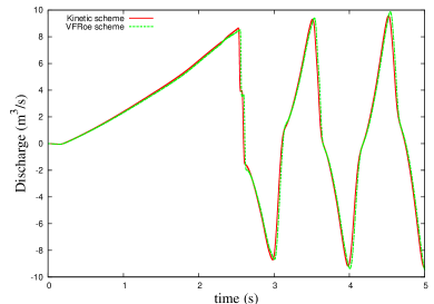
(a) Discharge

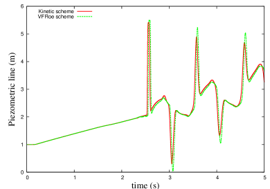
(b) Piezometric line

Figure 1: Comparison between the kinetic scheme and the upwinded VFRoe scheme at $x=0.5\,m$.

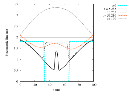
(a) Cell-centered friction

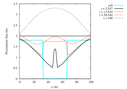
(b) Upwinded friction

Figure 2: Comparison of the cell-centered friction and upwinded friction for $K_{s}=100$.

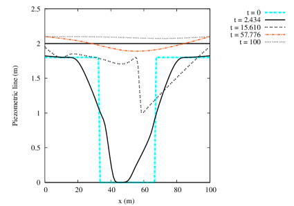
(a) Cell-centered friction

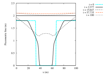
(b) Upwinded friction

Figure 3: Comparison of the cell-centered friction and upwinded friction for $K_{s}=10$.

References

• [1] C.Β Bourdarias, M.Β Ersoy, and S.Β Gerbi. A kinetic scheme for pressurized flows in non uniform closed water pipes. Monografias de la Real Academia de Ciencias de Zaragoza, 31:1–20, 2009.
• [2] C.Β Bourdarias, M.Β Ersoy, and S.Β Gerbi. A model for unsteady mixed flows in non uniform closed water pipes and a well-balanced finite volume scheme. International Journal On Finite Volumes, 6(2):1–47, 2009.
• [3] J.M. Greenberg and A.Y. LeRoux. A well balanced scheme for the numerical processing of source terms in hyperbolic equation. SIAM J. Numer. Anal., 33(1):1–16, 1996.
• [4] G.Β Dal Maso, P.Β G. Lefloch, and F.Β Murat. Definition and weak stability of nonconservative products. J. Math. Pures Appl., 74(6):483–548, 1995.
• [5] B.Β Perthame and C.Β Simeoni. A kinetic scheme for the Saint-Venant system with a source term. Calcolo, 38(4):201–231, 2001.
Refer to caption