Solar abundances and 3D model atmospheres

Abstract

We present solar photospheric abundances for 12 elements from optical and near-infrared spectroscopy. The abundance analysis was conducted employing 3D hydrodynamical (CO⁵BOLD) as well as standard 1D hydrostatic model atmospheres. We compare our results to others with emphasis on discrepancies and still lingering problems, in particular exemplified by the pivotal abundance of oxygen. We argue that the thermal structure of the lower solar photosphere is very well represented by our 3D model. We obtain an excellent match of the observed center-to-limb variation of the line-blanketed continuum intensity, also at wavelengths shortward of the Balmer jump..

1 Motivation

In recent years several solar abundances experienced a significant downward revision, among them major contributors to the overall solar metalicity ([Asplund et al. (2005), Asplund et al. 2005]). In part, the downward revision was attributed to the application of 3D model atmospheres. Due to the importance of the solar composition as a fundamental “yardstick” in astronomy, the CIFIST Team and its collaborators started an independent investigation of the solar abundances applying its self-developed analysis tools, in particular its own 3D model atmosphere code dubbed CO⁵BOLD ([Freytag et al. (2002), Freytag et al. 2002], [Wedemeyer et al. (2004), Wedemeyer et al 2004]). Table 1 summarizes the result for 12 elements in comparison to other works. Considering the latest compilation of Asplund and collaborators one can note a convergence towards a unique abundance set. However, there are still sizable differences present, in particular concerning the abundant element oxygen. Formally, the overlapping error bars could be taken to basically signal correspondence. However, one must keep in mind that certain systematics (observed spectra, oscillator strength, analysis methodology) are shared among all groups, and from that perspective differences are still on a rather high level. In this contribution we want to comment on a few of the lingering problems when it comes to the spectroscopic determination of solar abundances.

Table 1: Abundances derived by the CO⁵BOLD group in comparison to other compilations: AG89 [Anders & Grevesse (1989)]; GS98 [Grevesse & Sauval (1998)]; AGS05 [Asplund et al. (2005)]; AGSS09 [Asplund et al. (2009)]. El denotes the element, N the number of spectral lines used in our analysis. The last two rows give the total mass fraction of metals, and metals relative to hydrogen. Values set in italics refer to meteoritic abundances.

El	N	CO5BOLD	AG89	GS98	AGS05	AGSS09
Li	1	$1.03\pm 0.03$	$1.16\pm 0.10$	$1.10\pm 0.10$	$1.05\pm 0.10$	$1.05\pm 0.10$
C	43	$8.50\pm 0.06$	$8.56\pm 0.04$	$8.52\pm 0.06$	$8.39\pm 0.05$	$8.43\pm 0.05$
N	12	$7.86\pm 0.12$	$8.05\pm 0.04$	$7.92\pm 0.06$	$7.78\pm 0.06$	$7.83\pm 0.05$
O	10	$8.76\pm 0.07$	$8.93\pm 0.035$	$8.83\pm 0.06$	$8.66\pm 0.05$	$8.69\pm 0.05$
P	5	$5.46\pm 0.04$	$5.45\pm 0.04$	$5.45\pm 0.04$	$5.36\pm 0.04$	$5.41\pm 0.03$
S	9	$7.16\pm 0.05$	$7.21\pm 0.06$	$7.33\pm 0.11$	$7.14\pm 0.05$	$7.12\pm 0.03$
Eu	5	$0.52\pm 0.03$	$0.51\pm 0.08$	$0.51\pm 0.08$	$0.52\pm 0.06$	$0.52\pm 0.04$
Hf	4	$0.87\pm 0.04$	$0.88\pm 0.08$	$0.88\pm 0.08$	$0.88\pm 0.08$	$0.85\pm 0.04$
Th	1	$0.08\pm 0.03$	$0.12\pm 0.06$	${\it 0.09\pm 0.02}$	${\it 0.06\pm 0.05}$	$0.02\pm 0.10$
K	6	$5.11\pm 0.09$	$5.12\pm 0.13$	$5.12\pm 0.13$	$5.08\pm 0.07$	$5.03\pm 0.09$
Fe	15	$7.52\pm 0.06$	$7.67\pm 0.03$	$7.50\pm 0.05$	$7.45\pm 0.05$	$7.50\pm 0.04$
Os	3	$1.36\pm 0.19$	$1.45\pm 0.10$	$1.45\pm 0.10$	$1.45\pm 0.10$	$1.25\pm 0.07$
Z		0.0153	0.0189	0.0171	0.0122	0.0134
Z/X		0.0209	0.0267	0.0234	0.0165	0.0183

2 Sources of systematic uncertainties

While it may appear straight-forward to conduct a spectroscopic abundance determination there are a number of sources of systematic uncertainties which we list in the following. We comment on two selected aspects in more detail in subsequent sections. i) Are the selected lines appropriate? The issue of blending is an important and often difficult aspect to judge. The accuracy of atomic data is evidently also fundamental. ii) How accurate are our measurements of the lines’ equivalent width? The ever-lasting problem of the continuum placement constitutes a difficult to overcome limit to the achievable precision. Line shapes fitted to observations can mitigate but not eliminate this precision bottleneck. iii) How good are our model atmospheres, in particular 3D models? There have been long-lasting arguments about insufficient spatial resolution, and wavelength resolution when representing the energy exchange between gas and radiation field. iv) How great are the departures from local thermodynamic equilibrium? In particular, the poorly constraint efficiency of collisions with neutral hydrogen atoms in the calculation of the statistical equilibrium established a limit to which one can determine abundances from some lines. Prominent examples are the infrared triplet lines of neutral oxygen. v) Which solar spectrum is the solar spectrum? There are surprising differences among high quality solar atlases which need to be better understood – or even better overcome by a newer generation of atlases.

3 3D model properties

In this section we want to demonstrate that 3D models atmosphere have reached a high level of realism when it comes to the thermal structure of the lower photosphere – including temperature inhomogeneities due to granulation. Figure 1 illustrates the exceptional performance of our standard solar CO⁵BOLD model representing the center-to-limb variation of the solar radiation field on a spatial scale where granulation is not resolved. The calculation was done for a time series of 19 snapshots of the 3D flow field, whose intensity pattern was subsequently horizontally and temporally averaged. In the spectral synthesis calculations line blocking was accounted for by applying an ATLAS ([Kurucz (2005), Kurucz 2005]) Opacity Distribution Function with 1200 wavelength intervals, and 12 sub-intervals each. Fig. 1 shows the emergent intensity averaged over the 12 sub-bins. The same calculation was repeated for the 1D semi-empirical Holweger-Müller atmosphere ([Holweger & Müller(1974), Holweger & Müller 1974], HM). The overall match to the observations by the 3D model is remarkable, including the wavelength range in the Balmer continuum suffering from heavy line blocking. The precision is challenging the available observations and the performance of the HM model which was – at least in part – constructed to match the solar center-to-limb variation.

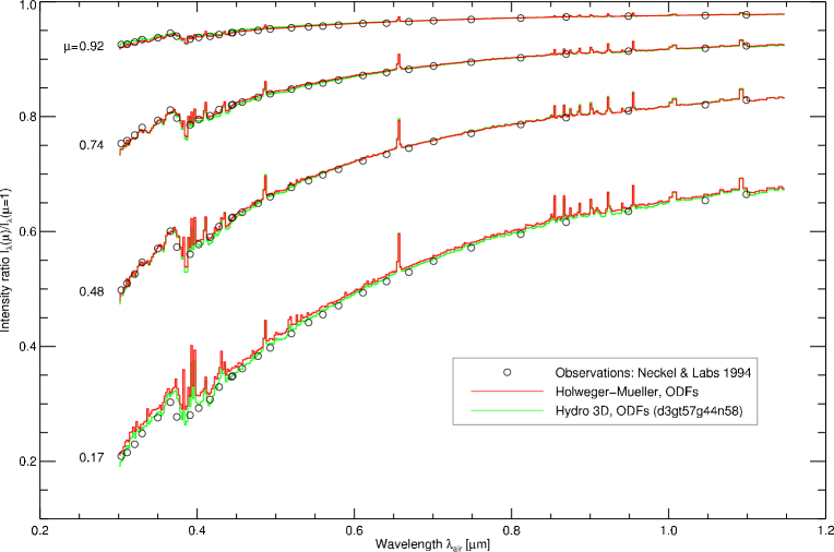
Figure 1: Center-to-limb variation with line blocking using ATLAS ODFs: for four heliocentric angles the intensity relative to disk-center is depicted as a function of wavelength.

4 Disentangling the [OI]+Ni I feature at 630 nm

The weak, forbidden oxygen line at 630 nm which is intimately blended with an even weaker line of neutral nickel, is considered as a prime abundance indicator of oxygen in the solar atmosphere since the line is immune to departures from LTE, and the blend lies in an otherwise rather clean part of the spectrum. The oscillator strength of the transitions of O and Ni are well determined so that one should expect that abundance determinations by various groups should largely coincide. The only remaining difficulty should be the separation of the total absorption in the feature into the contributions related to O and Ni. Figure 2 summarizes the results obtained during the last decade. All results have been normalized to the presently accepted values of the oscillator strength of the O and Ni transition. The depicted results were taken from: [Reetz (1999)], [Allende Prieto et al. (2001)], [Meléndez (2004)], [Ayres (2008)], [Caffau et al. (2008)], [Centeno & Socas-Navarro (2008)], and [Caffau et al. (2009)]. Stars indicate the application of theoretical model atmospheres in the analysis, squares the HM model. Different from the others the work of Centeno et al. is using spectro-polarimetric sunspot observations, and in this sense is particular. The lines of constant total equivalent width of the O+Ni feature were obtained with our spectral synthesis code and standard 3D solar model.

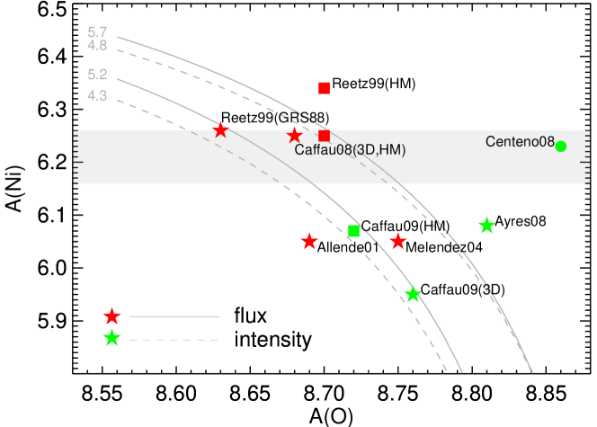
Figure 2: Oxygen and nickel abundances obtained by various groups from the 630 nm feature. “flux” refers to disk-integrated, “intensity” to disk-center spectra. The solid and dashed curves delineate the relation between O and Ni abundance at fixed total equivalent width of the feature (labels in mÅ). The grey bar indicates the currently accepted range of the Ni abundance from other Ni lines. Further details see text.

If all workers agreed in terms of model atmosphere and total equivalent width of the feature all results should line up on a curve of constant equivalent with in the O-Ni-abundance plane. However, even leaving aside the result of Centeno et al. a large scatter has to be noted. There is a noticeable influence of the applied model atmosphere, and also some effect of the assumed equivalent width. Most strikingly perhaps, the separation into the two components is far from unique. Here, the recent 3D based result of Caffau et al. (2009) indicates a particularly low Ni abundance. While it is difficult to reconcile with the presently accepted Ni abundance, it provides a striking illustration of the still lingering problems in the determination of solar photospheric abundances from spectroscopy.