Saving Entanglement via Nonuniform Sequence of $\pi$ Pulses

Abstract

We examine the question of survival of quantum entanglement between the bipartite states and multiparticle states like GHZ states under the action of a dephasing bath by the application of sequence of $\pi$ pulses. We show the great advantage of the pulse sequence of Uhrig [ 2007 Phys. Rev. Lett. 98 100504] applied at irregular intervals of time, in controlling quantum entanglement. In particular death of entanglement could be considerably delayed by pulses. We use quantum optical techniques to obtain exact results.

Contents

1. Introduction2

2. Dynamical decay of entanglement under dephasing3

3. Single qubit coherence $S(t)$5

4. Saving entanglement: numerical results6

5. Conclusions8

References9

1 Introduction

It is well known that the quantum entanglement deteriorates very fast due to environmental interactions and one would like to find methods that can save or at least slow down the loss of entanglement [1]. It is also now known that quantum entanglement can die much faster than the scale over which dephasing occurs [2]. For example the coherence of the qubit typically lasts over a time scale of the order of $T_{2}$ whereas the entanglement can exhibit sudden death and thus it is important to extend the techniques used for single qubits to bipartite and even multipartite systems. In this paper we examine how the pulse techniques which were developed to examine the issue of dephasing can help in saving the entanglement. The quantum dynamical decoupling [3, 4, 5] uses a sequence of control pulses to be used on the system at an interval much less than the time-scale of the bath coherence time. In this way, the coupling of the system to the bath can be time-reversed and thus canceled. Such non-Markovian approach has been successfully applied to two-level systems, harmonic oscillators [6]. A different approach was used in [7] where a control pulse was applied to a different transition rather than the relevant two-level transition. This technique shows that the control pulse causes destructive interference between transition amplitudes at different times which leads to inhibition of the spontaneous emission of an excited atom. Similar techniques could be useful to suppress the decoherence of a qubit coupled to a thermal bath. Other methods for protection against dephasing are known. These include application of fast modulations to the bath [8] as well as decoherence free subspaces [9]. The dynamical decoupling idea has been implemented in a few recent experiments [10] with excitons in semiconductors, with Rydberg atomic qubits, with solid state qubits and with nuclear spin qubits.

More recent developments primarily due to Uhrig [11, 12, 13, 14] go far beyond than what has been done earlier on dynamical decoupling. The dynamical decoupling schemes use a series of $\pi$ pulses applied at regular interval of times. The pulses reverse the evolution given by the Hamiltonian describing the interaction with a dephasing environment. This is because under a $\pi$ pulse the spin operator $S_{z}$ reverses sign. Uhrig discovered that $\pi$ pulses applied at irregular intervals of time are much more effective in controlling dephasing. The regular pulse sequence and the Uhrig sequence are given by

$$T_{j}=\frac{jT}{n+1},T_{j}=T\sin^{2}(\frac{\pi j}{2(n+1)}).$$ (1)

In this paper we focus on the utility of the sequence of pulses as discovered by Uhrig in saving quantum entanglement. Unlike other papers which focus on dephasing issues we concentrate on entanglement. This is important as the dynamical behavior of entanglement could be quite different than that of dephasing. We calculate the concurrence parameter [15] which characterizes the entanglement between the two qubits. We show the net time evolution of the concurrence parameter under the action of the Uhrig sequence of pulses and compare its evolution with the one given by when the uniform sequence of pulses is applied. We show the great advantage of the Uhrig sequence over the uniform sequence in saving entanglement. A very recent experiment [16] establishes the advantage of Uhrig’s sequence in lengthening the dephasing time of a single qubit. The organization of the paper is as follows: In Sec 2 we introduce the microscopic model of dephasing and calculate the relevant physical quantities under the influence of the control pulses. In Sec 3 we show how the coherent state techniques can be used to obtain the dynamical results. In Sec 4 we calculate the dynamics of entanglement and present numerical results. In Sec 5 we conclude with possible generalizations of our results on entanglement.

2 Dynamical decay of entanglement under dephasing

Let us consider two qubits in an entangled state [2] which in general could be a mixed state. In terms of the basis states for the two qubits, we choose the initial state as

$$\begin{array}[]{lcl}|1\rangle=|\uparrow\rangle_{A}\otimes|\uparrow\rangle_{B},|2\rangle=|\uparrow\rangle_{A}\otimes|\downarrow\rangle_{B},\vspace{.1in}\\ |3\rangle=|\downarrow\rangle_{A}\otimes|\uparrow\rangle_{B},|4\rangle=|\downarrow\rangle_{A}\otimes|\downarrow\rangle_{B}.\end{array}$$ (2)

$$\rho=\left(\begin{array}[]{cccc}a&0&0&0\vspace{.05in}\\ 0&b&z&0\vspace{.05in}\\ 0&z^{*}&c&0\vspace{.05in}\\ 0&0&0&d\vspace{.05in}\\ \end{array}\right).$$ (3)

The state (3) is positive and normalized if $a+b+c+d=1$ and $bc>|z|^{2}$. This state has the structure of a Werner state. For $a=d=0$; $b=c=|z|=1$, it represents a maximally entangled state. The amount of entanglement in the state is given by the concurrence given by

$$\begin{array}[]{lcl}C=\mbox{Max}\{0,\tilde{C}\},\vspace{0.1in}\\ \tilde{C}=2\{|\rho_{23}|-\sqrt{\rho_{11}\rho_{44}}\}=2|z|(1-r),\vspace{0.1in}\\ \displaystyle r=\frac{\sqrt{ad}}{|z|}.\end{array}$$ (4)

And therefore the state is entangled as long as $|z|$ is greater than $\sqrt{ad}$. Now under dephasing the diagonal elements $a$ and $d$ do not change. However the coherence in the qubit decays as $\exp[-t/T_{2}]$ and therefore the entanglement survives as long as $|z|\exp[-2t/T_{2}]-\sqrt{ad}>0$ and thus entanglement vanishes if $\displaystyle t>\frac{T_{2}}{2}\ln{\frac{|z|}{\sqrt{ad}}}$.

We would now examine how the action of pulses can protect the entanglement. We would calculate the time over which entanglement can be made to survive. For this purpose we need to examine the microscopic model of dephasing. We would make the reasonable assumption that each qubit interacts with its own bath. We could then examine the dynamics of the individual qubits and then obtain the evolution of the concurrence.

On a microscopic scale the dephasing can be considered to arise from the interaction of the qubit with a bath of oscillators i.e. from the Hamiltonian

$$H=\hbar\sum_{i}\omega_{i}a_{i}^{{\dagger}}a_{i}+\hbar S_{z}\sum_{i}g_{i}(a_{i}+a_{i}^{{\dagger}}),$$ (5)

where the $S_{z}$ is the $z$ component of the spin operator for the qubit and the annihilation and creation operators $a_{i}$, $a_{i}^{{\dagger}}$ represent the oscillators of the Bosonic bath. The bath is taken to have a broad spectrum. In particular for an Ohmic bath we take spectrum of bath as

$$J\rightarrow\sum_{i}|g_{i}|^{2}\delta(\omega-\omega_{i})=2\alpha\omega\Theta(\omega_{D}-\omega),$$ (6)

where $\omega_{D}$ is the cut off frequency. It essentially determines the correlation time of the bath. Such a bath leads to dephasing i.e. the spin polarization decays at the rate $T_{2}$. The dynamical decoupling schemes use a series of $\pi$ pulses applied at regular interval of times whereas Uhrig applies $\pi$ pulses at irregular intervals of time. Such nonuniformly spaced pulses are much more effective in controlling dephasing over a time interval determined by the cut off frequency and number of pulses. The regular sequence of pulses is more effective outside this domain. The pulses reverse the evolution given by the interaction part in the Hamiltonian (5) since under a $\pi$ pulse the spin operator $S_{z}$ reverses sign. The regular pulse sequence and the Uhrig sequence are given by equation (1). We need to calculate the dynamical evolution of the off diagonal element of the density matrix for the qubit. We work in the interaction picture hence the Hamiltonian (5) becomes

$$H=\hbar S_{z}\sum_{i}g_{i}(a_{i}e^{-i\omega_{i}t}+a_{i}^{{\dagger}}e^{i\omega_{i}t})=\hbar S_{z}B(t),$$ (7)

where $B(t)$ is the bath operator given by

$$B(t)=\sum_{i}g_{i}(a_{i}e^{-i\omega_{i}t}+a_{i}^{{\dagger}}e^{i\omega_{i}t}),$$ (8)

It is easy to see that the off diagonal element of the single qubit density matrix $\sigma$ is

$$\sigma_{\uparrow\downarrow}(t)=\Tr_{B}\langle\downarrow|U(t)\sigma_{B}\sigma(0)U^{{\dagger}}(t)|\uparrow\rangle,$$ (9)

where $\Tr_{B}$ is over the initial bath density matrix $\sigma_{B}$ and where

$$U(t)=T\exp\{-i\int_{0}^{t}S_{z}B(\tau)d\tau\}.$$ (10)

This can be simplified to

$$\begin{array}[]{lcl}\sigma_{\uparrow\downarrow}(t)=\sigma_{\uparrow\downarrow}(0)\Tr_{B}V_{-}(t)\sigma_{B}V_{+}^{{\dagger}}(t),\vspace{0.1in}\\ \hskip 32.52127pt=\sigma_{\uparrow\downarrow}(0)\langle V_{+}^{{\dagger}}(t)V_{-}(t)\rangle,\end{array}$$ (11)

where

$$V_{\pm}(t)=T\exp\{\mp\frac{i}{2}\int_{0}^{t}B(\tau)d\tau\}.$$ (12)

Thus we can write

$$\sigma_{\uparrow\downarrow}(t)=\sigma_{\uparrow\downarrow}(0)\zeta(t),$$ (13)

$$\begin{array}[]{lcl}\zeta(t)=\langle V_{+}^{{\dagger}}(t)V_{-}(t)\rangle,\vspace{0.1in}\\ \hskip 21.68121pt=\langle T\exp\{i\int_{0}^{t}B(\tau)d\tau\}\rangle.\end{array}$$ (14)

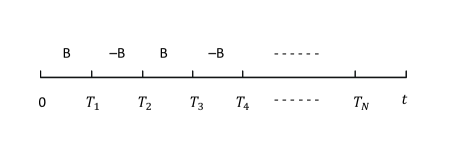
Figure 1: A sequence of $\pi$ pulses is applied at times $T_{j}$.

So far no approximation has been made. Now we incorporate the effect of pulses in the dynamical evolution of the single qubit coherence. Let us apply a sequence of $\pi$ pulses at times $T_{j}$ as shown in figure 1. At each $T_{j}$ the interaction Hamiltonian changes sign. This can be easily incorporated in the dynamics and the result is

$$\begin{array}[]{lcl}\zeta(t)=\langle W(t)\rangle,\vspace{0.1in}\\ W(t)=T\exp\{i\int_{0}^{t}B(\tau)f(\tau)d\tau\},\vspace{0.1in}\\ \displaystyle f(t)=\sum_{j=0}^{N-1}(-1)^{j}\theta(t-T_{j})\theta(T_{j+1}-t),\end{array}$$ (15)

where the step function $\theta(t)=1$ if $t>0,=0$, if $t<0$. It is especially instructive to use coherent state techniques to simplify the expression for $W$. We do this in the next section.

3 Single Qubit Coherence $S(t)$

We now examine the calculation of the function $W(t)$. We note that the bath operator $B(\tau)$ is such that the commutator $[B(\tau_{1}),B(\tau_{2})]$ is a c-number. In such a case it has been shown by Glauber [17] that the time ordering can be simplified. It can be shown that

$$W=\exp\{i\int_{0}^{t}B(\tau)d\tau f(\tau)\}\exp\{-\frac{1}{2}\int_{0}^{t}d\tau_{1}\int_{0}^{\tau_{1}}d\tau_{2}[B(\tau_{1}),B(\tau_{2})]f(\tau_{1})f(\tau_{2})\}.$$ (16)

Since $B$ is a Hermitian operator, the last exponential is just a c-number phase factor and hence

$$W=\exp(i\Phi(t))\exp\{i\int_{0}^{t}B(\tau)d\tau f(\tau)\},$$ (17)

$$\hskip 14.45377pt=\exp(i\Phi(t))\Pi_{j}\exp\{if_{j}a_{j}+if_{j}^{*}a_{j}^{{\dagger}}\},$$ (18)

where

$$f_{j}=g_{j}\int_{0}^{t}e^{-i\omega_{j}\tau}f(\tau)d\tau.$$ (19)

On using the Baker-Hausdorff identity (18) can be further simplified to

$$W=\exp(i\Phi(t))\Pi_{j}\exp\{if_{j}^{*}a_{j}^{{\dagger}}\}\exp\{if_{j}a_{j}\}\exp\{-\frac{1}{2}|f_{j}|^{2}\},$$ (20)

The thermal expectation value of $W$ can be easily obtained using for example the P-representation for the thermal density matrix [18]

$$\begin{array}[]{lcl}\displaystyle\rho_{thj}=\frac{1}{\pi n_{j}}\int\exp\{-\frac{|\alpha|^{2}}{n_{j}}\}|\alpha\rangle\langle\alpha|d^{2}\alpha,\vspace{0.1in}\\ \hskip 14.45377pt\displaystyle n_{j}=\frac{1}{e^{\beta\hbar\omega_{j}}-1}.\end{array}$$ (21)

Thus

$$W=\exp(i\Phi(t))\Pi_{j}\exp\{-\frac{1}{2}|f_{j}|^{2}\}\displaystyle\times\frac{1}{\pi n_{j}}\int\exp\{-\frac{|\alpha|^{2}}{n_{j}}\}\exp\{if_{j}^{*}\alpha^{*}+if_{j}\alpha\}d^{2}\alpha,\vspace{0.1in}\\$$ (22)

which on simplification reduces to

$$W=\exp(i\Phi(t))\Pi_{j}\exp\{-(n_{j}+\frac{1}{2})|f_{j}|^{2}\},$$ (23)

On using the form of $f_{j}$ and on introducing the spectral density of the bath oscillators, the expression (23) becomes

$$W=\exp(i\Phi(t))\exp\{-\int d(\omega)J(\omega)[n(\omega)+\frac{1}{2}]|f(\omega)|^{2}\},$$ (24)

where now

$$f(\omega)=\int_{0}^{t}e^{-i\omega\tau}F(\tau)d\tau.$$ (25)

The function $f$ can be simplified using the explicit form of $F(\tau)$:

$$f(\omega)=-i[1+(-1)^{N+1}e^{-i\omega t}+2\sum_{j=1}^{N}(-1)^{j}e^{-i\omega T_{j}}].$$ (26)

The result (23) is equivalent to equation (8) of Uhrig. We also note that results like (24) appear in the earlier literature [8] dealing especially with nonmarkovian master equations.

4 Saving Entanglement: Numerical Results

Since we work under the assumption that each qubit interacts with its own bath, the time dependent matrix elements of the density matrix in the basis (2) can be obtained by noting that the diagonal elements do not evolve under dephasing. The off diagonal element $\rho_{23}(t)$ is given by

$$\rho_{23}(t)=\rho_{23}(0)|\zeta(t)|^{2},$$ (27)

where $\zeta(t)$ is defined by equation (13) and its explicit form is given by equation (23). Thus

$$|\zeta(t)|^{2}=S(t)=\exp\{-2\int d\omega J(\omega)(n(\omega)+\frac{1}{2})|f(\omega)|^{2}\},$$ (28)

It can then be shown that the time dependence of the concurrence is given by

$$\begin{array}[]{lcl}C(t)=\mbox{Max}\{0,\tilde{C}(t)\},\vspace{0.1in}\\ \displaystyle\tilde{C}(t)=2|z|\{S(t)-r\},\vspace{0.1in}\\ \displaystyle r=\frac{\sqrt{ad}}{|z|}.\end{array}$$ (29)

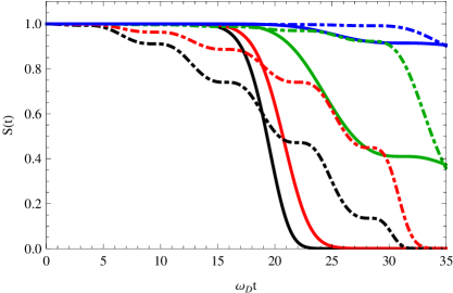
Figure 2: Signal vs time for $n=10$ at $T=0$. Solid lines for the optimized sequence, dotdashed lines for the equidistant sequence. From bottom to top the curves correspond to $\alpha=0.25,0.1,0.01,0.001$.

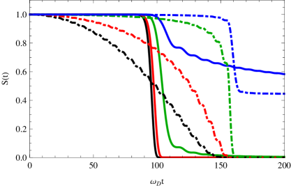
Figure 3: Signal vs time for $n=50$ at $T=0$. Solid lines for the optimized sequence, dotdashed lines for the equidistant sequence. From bottom to top the curves correspond to $\alpha=0.25,0.1,0.01,0.001$.

We next discuss the dynamical behavior of the entanglement. The function $f(\omega)$ has been evaluated by Uhrig. For the pulses applied at regular intervals and for $n$ even we have

$$|f(\omega)|^{2}=4\tan^{2}[\omega t/(2n+2)]\cos^{2}(\omega t/2)/\omega^{2}\hskip 7.22743pt\forall\hskip 7.22743ptn\hskip 7.22743pt\rm{even},$$ (30)

whereas for the Uhrig’s pulse sequence

$$|f(\omega)|^{2}\approx 16(n+1)^{2}J_{n+1}^{2}(\omega/2)/\omega^{2},$$ (31)

where $J_{n}$ is the Bessel function. The function $S(t)$ is shown in figures 2 and 3 for $n=10$ and $n=50$. The parameter $\omega_{D}^{-1}$ is a measure of the bath correlation time. These figures show that the entanglement lives much longer for Uhrig sequence of pulses applied at nonuniform intervals of time provided that $\omega_{D}t\leq 2n$. Thus entanglement can be made to live over times which could be several orders longer than the coherence time of the bath.

5 Conclusions

In conclusion we have considered how the effects of dephasing on the destruction of entanglement can be considerably slowed on by applying the sequence of $\pi$ pulses applied at time intervals given by Uhrig. We demonstrated this explicitly for the case of a mixed entangled state of two qubits. The sequence given by Uhrig is far better in controlling the death of entanglement compared to the sequence applied at regular intervals of time. These conclusions also apply to the multiparticle entangled state like the GHZ state

$$|\Psi\rangle=\frac{1}{\sqrt{2}}(|\uparrow\cdots\uparrow\rangle-|\downarrow\cdots\downarrow\rangle),$$ (32)

whose entanglement under dephasing would decay as the density matrix at time $t$ would be

$$\begin{array}[]{lcl}\displaystyle\rho(t)=\frac{1}{2}|\uparrow\cdots\uparrow\rangle\langle\uparrow\cdots\uparrow|+\frac{1}{2}|\downarrow\cdots\downarrow\rangle\langle\downarrow\cdots\downarrow|\vspace{0.1in}\\ \hskip 32.52127pt\displaystyle-\frac{1}{2}\exp\{-\frac{tN}{T_{2}}\}(|\uparrow\cdots\uparrow\rangle\langle\downarrow\cdots\downarrow|+c.c.).\end{array}$$ (33)

Under the application of $\pi$ pulses, the prefactor $\displaystyle\exp\{-\frac{tN}{T_{2}}\}$ would be replaced by $(S(t))^{N/2}$. Since $S(t)$ can be made close to unity for times even orders of the correlation time of the bath, the entanglement of the multiparticle GHZ state would survive over a long time. Note further that Uhrig’s work has been generalized to arbitrary relaxations [12]. Clearly these generalizations should be applicable to the considerations of entanglement. In particular we hope to examine the protection of Werner state against different models of environment.

Finally we note that our ongoing work also suggests how other methods like photonic crystal environment can be used to save entanglement.

References

References

- [1] Nielsen M A and Chuang I L 2004 Quantum Computation and Quantum Information (Cambridge University) Zurek W H 2003 Rev. Mod. Phys. 75 715
- [2] Yu T and Eberly J H 2004 Phys. Rev. Lett. 93 140404Yu T and Eberly J H 2006 Phys. Rev. Lett. 97 140403
- [3] Viola L and Lloyd S 1998 Phys. Rev. A 58 2733Viola L, Knill E, and Lloyd S 1999 Phys. Rev. Lett. 82 2417
- [4] Ban M 1998 J. Mod. Opt. 45 2315
- [5] Facchi P, Tasaki S, Pascazio S, Nakazato H, Tokuse A, and Lidar D A 2005 Phys. Rev. A 71 022302
- [6] Vitali D and Tombesi P 1999 Phys. Rev. A 59 4178
- [7] Agarwal G S, Scully M O, and Walther H 2001 Phys. Rev. Lett. 86 4271
- [8] Agarwal G S 1999 Phys. Rev. A 61 013809Kofman A G and Kurizki G 2001 Phys. Rev. Lett. 87 270405Kofman A G and Kurizki G 2004 Phys. Rev. Lett. 93 130406Linington I E and Garraway B M 2008 Phys. Rev. A 77 033831Gordon G 2008 Europhys. Lett. 83 30009
- [9] Palma G M, Suominen K, and Ekert A K 1996 Proc. R. Soc. London A 452 567Duan L-M and Guo G-C 1997 Phys. Rev. Lett. 79 1953Zanardi P and Rasetti M 1997 Phys. Rev. Lett. 79 3306Lidar D A, Chuang I L, and Whaley K B 1998 Phys. Rev. Lett. 81 2594Kwiat P G, Berglund A J, Altepeter J B, and White A G 2000 Science 290 498Ollerenshaw J E, Lidar D A, and Kay L E 2003 Phys. Rev. Lett. 91 217904
- [10] Kishimoto T, Hasegawa A, Mitsumori Y, Ishi-Hayase J, Sasaki M, and Minami F 2006 Phys. Rev. B 74 073202Minns R S, Kutteruf M R, Zaidi H, Ko L, and Jones R R 2006 Phys. Rev. Lett. 97 040504Fraval E, Sellars M J, and Longdell J J 2005 Phys. Rev. Lett. 95 030506Morton J J L, Tyryshkin A M, Ardavan A, Benjamin S C, Porfyrakis K, Lyon S A, Briggs G A D 2005 Nature Phys. 2 40
- [11] Uhrig G S 2007 Phys. Rev. Lett. 98 100504Khodjasteh K and Lidar D A 2005 Phys. Rev. Lett. 95 180501
- [12] Yang W and Liu R B 2008 Phys. Rev. Lett. 101 180403
- [13] Uhrig G S 2008 New J. Phys. 10 083024
- [14] Lee B, Witzel W M, and Sarma S D 2008 Phys. Rev. Lett. 100 160505
- [15] Wootters W K 1998 Phys. Rev. Lett. 80 2245
- [16] Du J, Rong X, Zhao N, Wang Y, Yang J, and Liu R B 2009 Nature 461 1265
- [17] Glauber R J 1965 in Quantum Optics and Electronics, eds C. DeWitt, A. Blandin and C. Cohen-Tannoudji (Gorden and Breach, Newyork) p 132
- [18] Glauber R J 1963 Phys. Rev. Lett. 10 84Sudarshan E C 1963 Phys. Rev. Lett. 10 277