Systematic approach to leptogenesis in nonequilibrium QFT:
self-energy contribution to the CP-violating parameter
Abstract
In the baryogenesis via leptogenesis scenario the self-energy contribution to the CP-violating parameter plays a very important role. Here, we calculate it in a simple toy model of leptogenesis using the Schwinger–Keldysh/Kadanoff–Baym formalism as starting point. We show that the formalism is free of the double-counting problem typical for the canonical Boltzmann approach. Within the toy model, medium effects increase the CP-violating parameter. In contrast to results obtained earlier in the framework of thermal field theory, the medium corrections are linear in the particle number densities. In the resonant regime quantum corrections lead to modified expressions for the CP-violating parameter and for the decay width. Most notably, in the maximal resonant regime the Boltzmann picture breaks down and an analysis in the full Kadanoff–Baym formalism is required.
pacs:
11.10.Wx, 98.80.CqI Introduction
From the theoretical point of view the baryogenesis via leptogenesis scenario Fukugita and Yanagida (1986) is a very attractive explanation of the observed baryon asymmetry of the Universe. One of its key ingredients is heavy Majorana neutrinos, whose CP–violating decays are responsible for the generation of a lepton asymmetry, i.e. for leptogenesis. The CP-violating parameter receives contributions from the vertex Fukugita and Yanagida (1986); Garny et al. (2009a) and self-energy Flanz et al. (1995); Covi et al. (1996); Pilaftsis (1997); Pilaftsis and Underwood (2004) diagrams. If the masses of the heavy neutrinos are strongly hierarchical, then the two contributions are comparable. However, if the mass spectrum is quasidegenerate then the self-energy contribution is resonantly enhanced and becomes considerably larger than the one from the vertex diagram. The resonant enhancement of the CP-violating parameter allows one to bring the scale of leptogenesis down to TeV Pilaftsis and Underwood (2004, 2005). This scenario is very interesting from the experimental point of view since it is potentially accessible in accelerator experiments Blanchet et al. (2009).
In state-of-the-art calculations the self-energy CP-violating parameter is evaluated in vacuum and then used to calculate the asymmetry generated by the decays of the heavy neutrinos in the hot and dense medium. In this approximation the possibly important medium effects are neglected from the very beginning. One can take them into account systematically by using the Schwinger–Keldysh/Kadanoff–Baym formalism Kadanoff and Baym (1962) or approximate self-consistent equations derived from the Kadanoff–Baym equations (see Covi et al. (1998); Buchmüller and Fredenhagen (2000); Giudice et al. (2004); Lindner and Müller (2006, 2008); De Simone and Riotto (2007a, b); De Simone (2008); Tranberg (2008); Hohenegger et al. (2008a); Anisimov et al. (2009); Gagnon (2009); Garny et al. (2009a); Kiessig and Plümacher (2009) for related work).
The Kadanoff–Baym formalism provides a powerful framework for studying nonequilibrium processes within quantum field theory. However, it is technically considerably more involved than the canonical Boltzmann approach. For this reason, we apply it here to a simple toy model which we have already used in Garny et al. (2009a) to investigate the vertex contribution. The Lagrangian contains one complex and two real scalar fields:
| (1) |
where denotes the complex conjugate of . Here and in the following we assume summation over repeating indices, unless otherwise specified. Despite its simplicity, the model incorporates all features relevant for leptogenesis. The real scalar fields imitate the (two lightest) heavy right-handed neutrinos, whereas the complex scalar field models the baryons. The symmetry, which we use to define “baryon” number, is explicitly broken by the presence of the last two terms, just as the symmetry is explicitly broken by Majorana mass terms in phenomenological models. Thus the first Sakharov condition Sakharov (1967) is fulfilled. The couplings model the complex Yukawa couplings of the right-handed neutrinos to leptons and the Higgs. By rephasing the complex scalar field at least one of the couplings can be made real. If the other one remains complex and there is CP-violation, as is required by the second Sakharov condition. In vacuum the self-energy contribution to the CP-violating parameter is given by:
| (2) |
where is the decay width of the heavy scalar . Note that the expression (2) has been obtained using the formalism developed in Pilaftsis and Underwood (2004). The formalism employed in Anisimov et al. (2006) leads to a slightly different expression for the CP-violating parameter (see Appendix A for more details). The required deviation from thermal equilibrium is caused by the rapid expansion of the Universe. Thus the third Sakharov condition is fulfilled as well. Finally, the quartic self-interaction term in (I) plays the role of the Yukawa and gauge interactions in established models – it brings the “baryons” to equilibrium. The renormalizability of the theory requires the presence of some additional terms, which are accounted for by .
Here, we study the self-energy contribution to the CP-violating parameter in the hierarchical and quasidegenerate cases using the Schwinger–Keldysh/Kadanoff–Baym formalism as starting point. To make the discussion less technical we give the details of the calculation in the appendixes, whereas in the main body of the paper we sketch the derivation and present the results.
-
(i)
As we argue in Sec. III, the formalism is free of the double-counting problem typical for the canonical Boltzmann approach. In other words the structure of the equations automatically ensures that the asymmetry vanishes in thermal equilibrium and no need for the real intermediate state (RIS) subtraction arises. This property has already been observed in case of the vertex contribution.
-
(ii)
The medium corrections to the CP-violating parameter are only linear in the particle number densities. That is, our result differs from that obtained previously in the framework of equilibrium thermal field theory by replacing the zero temperature propagators with finite temperature propagators in the matrix elements used in the Boltzmann equation.
-
(iii)
For scalars the medium effects always increase the CP-violating parameter, which in turn leads to an enhancement of the generated asymmetry.
-
(iv)
The canonical expression for the CP-violating parameter is only applicable in the hierarchical case even though it does not diverge in the limit of equal masses. For quasidegenerate masses one has to take into account quantum corrections to the effective masses and decay widths of the heavy particles in medium, which leads to a modified expression for the CP-violating parameter.
-
(v)
In the resonant regime quantum corrections also lead to an enhancement of the total in-medium decay widths. This results in a faster decay of the heavy particles and can increase the importance of the washout process.
-
(vi)
In the maximal resonant regime the Boltzmann picture breaks down and we argue that an analysis in the full Kadanoff–Baym formalism is required.
In Sec. IV we present numerical solutions of the quantum-corrected Boltzmann equations, and discuss the quantitative impact of medium effects on the final asymmetry within the toy model. Finally, in Sec. V, we summarize the results and present our conclusions.
II Kinetic equation
The canonical approach to the calculation of the asymmetry generated at the epoch of leptogenesis is based on the use of Boltzmann equations. In the expanding Universe the Boltzmann equation for the toy-baryon distribution function can be written in the form Kolb and Turner (1990)
| (3) |
where all functions are evaluated at the same point of the phase-space, is the covariant derivative and the quantities correspond to the gain and loss terms. For decays into a pair of toy-baryons they are given by
| (4a) | ||||
| (4b) | ||||
where is the invariant momentum-space volume element. The analogous equations for the toy-antibaryon distribution function and the corresponding quantities can be obtained from (3) and (4) by replacing the subscript with .
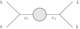
At tree level, see Fig. 1 (a), the decay is CP-conserving, that is . There are two distinct contributions to the CP-violating parameter, the vertex Fukugita and Yanagida (1986); Garny et al. (2009a) and the self-energy Flanz et al. (1995); Pilaftsis (1997) ones. The leading-order self-energy contribution is generated by the one-loop self-energy diagram depicted in Fig. 1 (b).
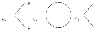
Only the diagram where the initial () and intermediate () toy-Majoranas are different () contribute to the CP-violating parameter. Summing the tree-level and the “off-diagonal” one-loop self-energy amplitudes one obtains and . In the corresponding expressions for the “antibaryons” the signs in front of are reversed. If these amplitudes are now substituted into and one finds that a nonzero asymmetry is generated even in thermal equilibrium, which is inconsistent with the CPT symmetry. This is a manifestation of the so-called double-counting problem typical for the canonical Boltzmann formalism. Let us briefly explain what that means. An inverse decay immediately followed by a decay is equivalent to the two-body scattering process where the intermediate toy-Majorana is on the mass shell. That is, the same contribution is taken into account twice: once when the decay and inverse decay processes are considered and once when the two-body scattering processes are considered. This problem is usually solved by subtracting the contribution of the on-shell intermediate state to the scattering amplitude Pilaftsis (1997); Pilaftsis and Underwood (2004). Roughly speaking, after the subtraction the amplitude of the inverse decay process also becomes proportional to , which ensures that in thermal equilibrium no asymmetry is produced due to detailed balance.
In the canonical bottom-up approach, which has been outlined above, one uses elements of the S-matrix (in-out formalism) to calculate the functions . In contrast to that, in the top-down approach based on the Schwinger–Keldysh/Kadanoff–Baym Schwinger (1961); Keldysh (1964); Bakshi and Mahanthappa (1963); Danielewicz (1984a); Chou et al. (1985); Calzetta and Hu (1988); Ivanov et al. (2000); Knoll et al. (2001); Blaizot and Iancu (2002); Berges and Müller (2002); Berges and Borsanyi (2006); Weinstock (2006); Carrington and Mrowczynski (2005); Fillion-Gourdeau et al. (2006) formalism, the functions can be identified with self-energies and are derived, using nonequilibrium field theory techniques (see e.g. Berges (2004a); Carrington and Mrowczynski (2005)), from the two-particle-irreducible (2PI) effective action111Note that there exists a straightforward generalization to a hierarchy of so-called nPI effective actions Berges (2004b). In general, for systems far from equilibrium and for strong couplings the 2-body decay is best described using 3PI. However, for leptogenesis, 2PI is sufficient since the CP-violation is dominated by the leading loop diagrams. Cornwall et al. (1974) formulated on the closed real-time path (in-in formalism).
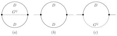
A two-loop contribution to the effective action and the corresponding contribution to the self-energy of the “baryons” are presented in Fig. 2 (a) and Fig. 2 (c) respectively. Wigner-transforming the self-energy we obtain Garny et al. (2009a)
| (5a) | ||||
| (5b) | ||||
where , is the covariant generalization of the Dirac -function and and are the Wightman propagators of the real and complex fields respectively. In the Boltzmann-limit the latter are related to the distribution function by
| (6) |
where in the quasiparticle approximation (see Garny et al. (2009a) for more details) the spectral function reads
| (7) |
In the same approximation the Wightman propagators of the toy-antibaryons, , can be obtained from (6) by replacing with .
If the real scalar fields would not mix, i.e. if the off-diagonal components of the Wightman propagator were equal to zero, we could also write analogous expressions for the diagonal components:
| (8) |
with the spectral function given by
| (9) |
Because of the presence of the Dirac -function in (7) and (9) the integrations over and could then be performed trivially and we would recover (4) in the CP-conserving limit.
A nonzero toy-baryon asymmetry can be generated only if . Comparing (5) and (5) we see that if initially the system is symmetric, i.e. , this amounts to the requirement that the Hermitian matrix has complex off-diagonal components. If the off-diagonal components peak on the mass shell of the quasiparticle species, i.e. if they can be represented in the form
| (10) |
then the generation of the asymmetry can be analyzed in terms of CP-violating parameters. Substituting (10) into (5) we find
| (11) |
To calculate the decomposition coefficients we use the nonequilibrium formulation of the Schwinger-Dyson equation, which is discussed in the following section.
III CP-violating parameter
Just like in the canonical analysis Pilaftsis (1997); Pilaftsis and Underwood (2004) the starting point of our analysis is the Schwinger–Dyson equation
| (12) |
where is the full dressed propagator of the “heavy neutrinos”, is the diagonal propagator of the free fields and is the self-energy. In the two-loop approximation, see Fig. 2, the self-energy is given by
| (13) |
where is the full propagator of the complex scalar field and . Note that the arguments of the two-point functions and self-energy are defined on the positive and negative branches of the Schwinger–Keldysh closed real-time contour Schwinger (1961); Keldysh (1964); Bakshi and Mahanthappa (1963); Danielewicz (1984a); Chou et al. (1985); Calzetta and Hu (1988) shown in Fig. 14.
If we multiply (12) by from the right, decompose the full propagator and the self-energy into statistical and spectral components and integrate over the contour, we obtain a system of so-called Kadanoff–Baym equations for the statistical propagator and spectral function (see Appendix B). Within leptogenesis, the light particle species are usually assumed to be very close to kinetic equilibrium. Translated to the toy model, this means that the toy-baryons described by the propagators and are close to equilibrium. In this case, one can approximate the full Kadanoff–Baym equations by quantum kinetic equations, and find approximate analytic solutions of these equations. Using these solutions, it is possible to explicitly obtain the decomposition coefficients , which then yield the corresponding CP-violating parameters as described above. This approach is pursued in Appendix B. In this section we will use an alternative approach, which essentially relies on the same assumptions, but is somewhat more elegant.
In the following, we use a compact matrix notation for Eq. (12), where we denote the matrices by a hat, e.g. . Let us split the self-energy matrix into the diagonal and off-diagonal components and introduce a diagonal propagator defined by the equation
| (14) |
Subtracting (14) from (12) we find
| (15) |
Multiplying (15) by from the left, by from the right and integrating over the contour we obtain a formal solution for the full nonequilibrium propagator:222Here, we implicitly assume that the correlators are diagonal at the initial time of the closed time path evolution. Since we consider the kinetic limit later on, for which the initial time is formally sent to negative infinity, the results are not affected.
| (16) |
The invariant volume element, , where , ensures that (III) can be applied to the analysis of out-of-equilibrium dynamics not only in Minkowski, but also in a general curved space-time Hohenegger et al. (2008a). Using the decomposition
| (17) |
and an analogous relation for the self-energy we can split (III) into spectral and statistical components. These are related to the Wightman propagators by
| (18) |
Because of the function in the decomposition of the two-point function and self-energy the integrals over the closed-time-path contour in (III) reduce to integrals over parts of the plane; see Appendix C. Introducing the retarded and advanced propagators,
| (19a) | ||||
| (19b) | ||||
and also the retarded and advanced self-energies we can represent the resulting expressions as integrals over the whole plane. Finally, building the linear combinations (18) we find for the Wightman propagators
| (20) |
Using (18) and (19) we can also derive formal solutions for the retarded and advanced propagators from (III). They read
| (21) |
In thermal equilibrium the two-point functions and self-energies in (III) and (III) depend only on the relative coordinate, , and are independent of the center coordinate, , i.e. are translationally invariant. As discussed above, we expect that the deviations from equilibrium are moderate. In this case, one can perform a gradient expansion of the two-point functions and the self-energies in the vicinity of keeping only the leading terms. Performing the Wigner transformation, i.e. the Fourier transformation with respect to the relative coordinate (see Appendix B) we trade the relative coordinate for a coordinate in momentum space. Effectively, the Wigner transformation replaces the coordinate-space arguments of each two-point function in (III) and (III) by the phase-space coordinates and “removes” the double integration; see Appendix C. Combining the Wigner transforms of (III) and (III) we find for the full Wightman propagators
| (22) |
where all the functions are evaluated at the same point of the phase-space. The term proportional to describes scattering Špička and Lipavský (1995); Köhler (1992); Köhler and Malfliet (1993); Köhler and Morawetz (2001); Morozov and Röpke (2006a, b); Weinstock (2006); Carrington and Mrowczynski (2005); Fillion-Gourdeau et al. (2006) and is irrelevant for us at the moment. Contracting the decay term with the product of the couplings in (5) and using that, by construction, the propagators are diagonal and off-diagonal, we find
| (23) |
where
| (24) |
In (24) and all the equations below we implicitly assume summation over all .
A very important feature of (23) is that the loop corrections are the same for both the gain and loss terms (i.e. for the and components), respectively. To obtain an equivalent result in the canonical approach one needs to apply the real intermediate state subtraction procedure Pilaftsis (1997); Pilaftsis and Underwood (2004). This means that, here, the structure of the equations automatically ensures that no asymmetry is generated in thermal equilibrium. Stated differently, the formalism is free of the double-counting problem and no need for RIS subtraction arises. This conclusion is in accordance with the corresponding result for the vertex contribution to the CP-violating parameter Garny et al. (2009a).
Contracting the decay term with the product of the couplings in (5) we obtain an expression similar to (23) but now with
| (25) |
From Eq. (5), we see that the rates for the decays and differ from each other only if . The corresponding CP-violating parameter is given by
| (26) |
The first terms in (24) and (25) are equal and cancel out in the difference of and . Therefore, in agreement with (11), the CP-violating parameter can be expressed as
| (27) |
Equation (23) also provides us with an expression for the total in-medium decay widths of the heavy particles:
| (28) |
where are the corresponding tree-level decay widths in vacuum.
The CP-violating parameter (27) is a function of the space-time coordinate and four-momentum . Note that in general does not need to be on-shell. The on-shell condition is determined by the diagonal components of the full propagator. The CP-violating parameter carries information about the off-diagonal components, compare Eq. (10). Therefore, the conventional, “on-shell”, interpretation of (27) is only applicable if the off-diagonal components of the full propagator peak at the same values of the momentum as the diagonal ones. Furthermore, if we want to use the Boltzmann equations for to calculate the asymmetry, then the mass spectra of the diagonal () and full () propagators must be sufficiently close.
The value of the CP-violating parameter depends on the masses of the heavy species and the coupling constants or, alternatively, the decay widths . It is useful to discriminate between three cases, namely
| (29) | ||||
where . As we will argue in the following, the generation of the asymmetry can be studied approximately in the Boltzmann picture using the above CP-violating parameter in the strongly hierarchical and resonant cases, but not in the maximal resonant case.
III.1 Strongly hierarchical case
In this subsection, we derive the CP-violating parameter in the strongly hierarchical limit, . As we shall see later, in the hierarchical case the denominator in Eq. (27) is close to unity. The same is true for the denominator of (28). Therefore the in-medium decay widths coincide with the tree-level ones. For the CP-violating parameter we obtain
| (30) |
It only remains to calculate the last term in (30). Let us first analyze the self-energy . In a “baryonically” symmetric configuration the particles and antiparticles are interchangeable, so that (see Appendix F for a proof). In the following, we will use that the baryon asymmetry is small, i.e. . In this case the two terms of (13) combine to a symmetric matrix which is proportional to . To obtain we decompose this matrix into a statistical and spectral part, multiply the spectral part with and perform the Wigner transformation. The result reads
| (31) |
where the superscript ‘s’ refers to the “baryonically” symmetric configuration and is the statistical propagator of the complex field. In the quasiparticle approximation . The retarded and advanced propagator of the complex scalar field can be represented in the form , where in the quasiparticle approximation is given by (7) and ; see Eq. (192). Consequently, in the symmetric configuration the retarded self-energy is given by a linear combination of two real-valued symmetric matrices:
| (32) |
where, to shorten the notation, we have introduced
| (33) |
For a homogeneous and isotropic system the one-particle distribution functions depend only on the Lorentz-invariant product , where is the particles’ momentum and is the (constant) four-velocity of the medium with respect to the chosen frame of reference. Using this property, in Appendix G we evaluate on the mass shell of the ’th quasiparticle:
| (34) |
where . Here, and are the components of the four-momentum of the heavy scalar in the rest-frame of the medium, and . For massless toy-baryons in vacuum . Taking a nonzero toy-baryon mass into account yields . In medium (symmetric case), we find using Eq. (34)
| (35) |
where and are the largest and smallest kinematically allowed energies of the light scalars produced in the decay .
As we show in Appendix B, analogously to (32) the Wigner transforms of the retarded and advanced propagators can be represented as linear combinations of two Hermitian matrices. Applied to the matrix this implies that it splits into two real-valued diagonal matrices:
| (36) |
In the hierarchical case we can neglect the finite decay widths of the quasiparticle species and approximate by (9). It diverges on the mass shell of the ’th quasiparticle and is zero everywhere else. Because of the presence of in (23), the CP-violating parameter (30) must be evaluated on the mass shell of the ’th quasiparticle. Since the product of and vanishes in the quasiparticle approximation, we conclude that only the term contributes. It is given by Hohenegger et al. (2008a)
| (37) |
In vacuum the tree-level decay width of the heavy species is given by . Therefore, we can rewrite the diagonal components of the spectral self-energy in the form .
In the hierarchical case . Substituting (32) and (36) into (30), and evaluating the momentum on-shell, , we then obtain for the CP-violating parameter333Note that, by setting , we neglect possible off-shell effects (see Appendix A). This is a good approximation if , which is the case in the strongly hierarchical case.
| (38) | ||||
For massless toy-baryons in vacuum and we recover the classical result (2). In the strongly hierarchical limit, one can neglect the decay width in the denominator of (38). In this case,
| (39) |
This result is identical to the one for the vertex contribution Garny et al. (2009a). The CP-violating parameter is given by a sum of vacuum and medium contributions. From Eq. (35), we find that the medium contributions are proportional to the one-particle distribution function, which is positive. Hence, for the scalar toy model and the strongly hierarchical limit considered here, the self-energy contribution to the CP-violating parameter is always enhanced by the medium effects.
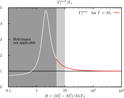
Note that the medium contribution depends only on the distribution function of the toy-baryons and is independent of that of the toy-Majoranas. Since we expect the light scalars to be close to kinetic equilibrium at all times, it is instructive to estimate the size of the corrections in thermal equilibrium. In the hierarchical limit the asymmetry is predominantly generated by the decay of the lighter toy-Majorana. Inserting a Bose–Einstein distribution (BE) or a Maxwell–Boltzmann (MB) distribution function we obtain for the ratio of the corresponding CP-violating parameter and its vacuum value:
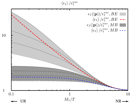
The temperature- and momentum dependence of the medium correction in the range of typical momenta is shown in the shaded areas in Fig. 3 for the BE and MB cases, respectively. We also show the CP-violating parameter obtained by averaging Eq. (38) over the momentum . As expected, .
As we have argued above, the conventional interpretation of the CP-violating parameter is only possible if the off-diagonal components of the full propagator peak at the same values of the momentum as the diagonal ones.
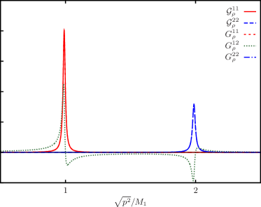
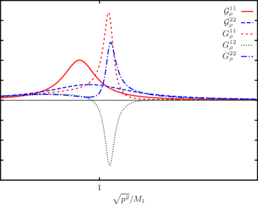
In Fig. 4 we show the qualitative behavior of the components of the diagonal and full spectral functions as obtained from Eq. (B.4). As one can infer from the plot, the off-diagonal components do peak at the same values of the momentum argument as the diagonal ones. Furthermore, the peaks of and are almost indistinguishable. Therefore we can use the Boltzmann equations for the diagonal propagators to calculate the asymmetry.
To conclude this section, let us estimate the range of applicability of (38). It was obtained by approximating the denominator of (27) by unity. Since and we obtain
| (40) | ||||
Evaluated on the mass-shell of the ’th quasiparticle, the retarded propagator,
| (41) |
is of the order of the inverse splitting of the squared masses, . Thus the contribution is of order of , whereas the contribution involving is of order of .
III.2 Resonant case
If the spectrum of heavy (toy-)neutrinos is quasidegenerate, , the CP-violation parameter (2) predicts a resonant enhancement of the generated asymmetry, known as resonant leptogenesis Pilaftsis and Underwood (2004). Because of the enhancement, this scenario allows to circumvent the lower bound on the lightest right-handed neutrino mass typical for thermal leptogenesis Davidson and Ibarra (2002). Therefore, resonant leptogenesis is discussed as a possibility to evade constraints from the production of gravitinos due to their impact on big bang nucleosynthesis, associated with the necessity of reheating temperatures well above in the hierarchical case Giudice et al. (2008). Furthermore, it has even been argued that the resonant enhancement could lower the scale of right-handed neutrinos to the TeV range, with possible implications for collider experiments Blanchet et al. (2008, 2009); Dar et al. (2006); Frere et al. (2009). Therefore, it is important to check whether the conventional Boltzmann treatment which uses the canonical CP-violation parameter (2) agrees with the nonequilibrium field theory description in the quasidegenerate limit.
Let us start by noting that the result (38) for the CP-violating parameter in the strongly hierarchical limit formally agrees with the canonical result (2) even in the quasidegenerate case. However, its derivation did involve approximations that break down in the resonant case. We will now revisit this derivation, starting from Eq. (27), without the above approximations. As explained, the denominator of (27) can significantly deviate from unity in the resonant case, which we take into account here. Using Eq. (40) we find
| (42) |
Note again that we implicitly assume summation over in the enumerator and the denominator, respectively.
From Eqs. (40) and (32) we see that the denominator of (42) involves the self-energy , which is logarithmically UV-divergent. It can be renormalized by including a mass counterterm. As shown in Appendix D, this amounts to the replacements , and
| (43) |
For our purposes, it is convenient to use an on-shell renormalization scheme, for which
| (44) |
where denotes the dispersive part of the renormalized self-energy in vacuum.
Note that, in vacuum, the self-energy is time-independent and depends only on due to Lorentz invariance (there is no medium which singles out a preferred frame). Note also that the six independent counterterms described by the symmetric two-by-two matrices and are fully determined by the above renormalization conditions. For the renormalized self-energy in medium, we find (see Appendixes A and G)
| (45) | |||||
where, in the medium rest-frame (for ),
It is also straightforward to generalize the decomposition (32) to the renormalized case. While the imaginary part is not affected, we define (for )
| (47) |
Since we will only use the renormalized quantities from now on, we omit the superscript ‘ren’ for brevity. Then, using also (36), we find
| (48) | ||||
where and . Note that , which is given by (41), as well as its real and imaginary components, and , also contain the renormalized self-energy.
The propagators and the components of the self-energy in (48) are functions of the center coordinate and the four-momentum . In general, the components of are not related by the on-shell condition, so that (48) describes CP-violating effects in the decays of on- and off-shell toy-Majoranas. However, if then the largest contribution to comes from on-shell momenta. The in-medium dispersion relation is determined by the equation444The contributions of off-shell momenta can be partially taken into account by evaluating the CP-violating parameter at a complex value of determined by Anisimov et al. (2006). However, note that this approach (just as the original result (48), which is valid also off-shell) requires the use of an off-shell generalization of the Boltzmann equations.
| (49) |
An effective, momentum-dependent mass can be defined by the relation , which implies
| (50) |
By means of Eq. (50) we take the mass-shift of the in-medium masses, , into account. In a thermal medium, they correspond to thermal masses. Even though the mass shifts are small compared to , they can be important for the mass difference in the quasidegenerate case.
Finally, we evaluate Eq. (48) for , using Eqs. (41) and (36). We obtain the following result for the CP-violating parameter:
| (51) | ||||
where encodes the medium correction discussed already in the hierarchical case, obtained by replacing in (35). The denominator consists of two contributions, weighted by the parameters
| (52) | |||||
related to the CP-violating phase . Furthermore, the degeneracy parameter,
| (53) |
is given by the difference of the in-medium (“thermal”) masses of the heavy toy-neutrinos, plus logarithmic corrections (here we display the superscript ‘’ again for clarity):
| (54) | |||||
As we have already mentioned, the resonance effects modify not only the CP-violating parameters, but also the total decay widths of the heavy particles; see Eq. (28). Using the functions and definitions introduced above we can write the in-medium decay widths in the form
| (55) | |||
In the limit , the CP-violating parameter (51) converges toward the result (38) for the hierarchical case. Our result for the resonant case, Eq. (51), describes the leading corrections when the above ratio becomes sizable. However, one should keep in mind that, in the “maximal resonant” case, where the decay width is comparable to the mass difference, the Boltzmann picture breaks down. The following simple argument supports this statement: To a good approximation the spectral functions of the heavy fields have a Breit-Wigner shape. To evaluate the gain and loss terms (5) we have to integrate over the frequency of the heavy particles’ propagator. If the distance between the peaks of the spectral function is considerably larger than the decay widths, the integration reduces to two independent integrations in the vicinities of the corresponding mass shells. Thus, we can identify two independent quasiparticle excitations with the corresponding distribution functions and and the CP-violating parameters and which contribute to the generation of the asymmetry. On the other hand, if the decay width is comparable to the difference of the masses, then the peaks of the spectral functions overlap and neither the distribution functions, nor the CP-violating parameters, are well-defined.
In Fig. 5 we present the qualitative behavior of the diagonal and off-diagonal components of the full and diagonal spectral functions and . As one can infer from the plot, the off-diagonal components of the full spectral function no longer have two pronounced peaks. Thus, it is not possible to define two CP-violating parameters. The shape of the diagonal components deviates from the Breit-Wigner one, and the positions of the peaks of are shifted as compared to those for the diagonal spectral function . In other words, using the Boltzmann equation for the diagonal propagators to calculate the generated asymmetry is no longer a good approximation because of the off-shell effects. Moreover, since the microscopic time scales and the macroscopic time scales can be of the same order of magnitude in the “maximal resonant” regime, the memory effects can play an important role. Thus we conclude that in this case, one should use the quantum kinetic equations discussed in Appendix B, which take off-shell effects into account, or even the full nonlocal quantum evolution equations discussed in Appendix E, which also capture memory and correlation effects.
With these considerations in mind, let us now analyze the Kadanoff–Baym/Schwinger–Keldysh result (51) for the CP-violating parameter in the resonant (but not maximal resonant) regime, for some particular cases of interest. For definiteness we concentrate here on , i.e. assuming that . In terms of the ratio
| (56) |
the condition of validity for the Boltzmann-treatment can be expressed as . The hierarchical limit corresponds to . In the following we study the leading corrections in .
In order to separate medium and resonance corrections, we first consider the vacuum limit . The renormalization prescription Eqs. (III.2) ensures that , i.e. and are the on-shell masses in vacuum. Furthermore, adopting the scheme (III.2) also implies that and
| (57) |
Therefore, in the vacuum limit the degeneracy parameter is given by
| (58) |
For , the loop correction can be safely neglected. Thus, in the vacuum limit the CP-violating parameter is approximately given by
| (59) |
Compared to the conventional result (2) the width in the denominator is effectively changed according to . Since , this means that for fixed values of and the result above is always larger compared to the conventional one. This property may be attributed to the fact that the Kadanoff–Baym formalism takes a resummation of resonant contributions into account. Note that, if taken at face value, the expression (III.2) for formally has a peak at , with maximum and width . The width reduces to zero in the limit of vanishing CP-violation, , although the peak value remains finite. On the contrary, for the conventional result (2) one has , and a width . However, we stress that the result should only be trusted in the regime where , and can be modified significantly by medium effects.
There are two sources of medium corrections in the resonant case. The first is the contribution from the spectral (imaginary) part of the self-energy loop, given by in Eq. (51). This contribution is known already from the hierarchical case; see Eq. (38) as well as Fig. 3. The second contribution stemming from the real part of the self-energy loop, given by , enters via the thermal masses and also via the “logarithmic” corrections.
For illustration, we insert a Bose-Einstein distribution for and (with ) in the expression for in Eq. (III.2). In the limit , we obtain
| (60) |
| (61) | |||||
The term in square brackets is of second order in the mass-squared difference and can be neglected. Assuming in addition , the degeneracy parameter is approximately given by
| (62) |
In the quasi degenerate limit it is plausible to assume that also the couplings are quasi degenerate, . In this case, the thermal corrections stemming from the dispersive part of the self-energy cancel approximately. In general, the thermal corrections could also be larger than the mass-splitting of the vacuum masses. If the vacuum masses are quasi degenerate, this would destroy the resonance condition. However, also the opposite case is possible, namely could become tiny due to a cancellation of the vacuum masses and the thermal corrections for a certain temperature. Then the resonant enhancement would occur only close to this particular temperature. We do not pursue these possibilities further here. Assuming, for simplicity, that the thermal contributions in Eqs. (III.2) and (62) are subdominant, we can summarize the results for the medium- and resonance corrections to the CP-violating parameter as follows:
| (66) |
The first two expressions follow directly from Eq. (2) and Eq. (38), respectively. The third one approximates the resonant result, Eq. (51), for .
In Fig. 6 we show the ratio of the expressions for the CP-violating parameter, Eq. (51), which includes medium and resonance corrections, and Eq. (38), which includes only medium corrections, for several values of the degeneracy parameter .
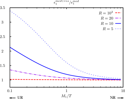
Large values of correspond to the hierarchical case and there is no difference between the two approximations. On the other hand, for small values of the corrections are substantial. For instance for the expression without resonance corrections underestimates the CP-violating parameter by a factor of two at high temperatures.
Since typically most of the asymmetry is generated at , it is instructive to look at the CP-violating parameter as a function of the degeneracy parameter at .
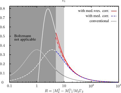
In Fig. 7 we present the -dependence of the conventional vacuum approximation for the CP-violating parameter, Eq. (2), the hierarchical approximation in medium, Eq. (38), and the resonant expression, Eq. (51), respectively. Very large values of correspond to . In this case the resonance effects are suppressed and all three expressions go to zero . For smaller values of we observe a significant deviation of the CP-violating parameter from its vacuum value, which is due to medium effects. Finally for even smaller values of the resonant effects become important and we observe a deviation of the CP-violating parameter from its value calculated in the hierarchical approximation.
The effective decay widths are also enhanced by the medium and resonance effects. The enhancement increases with the temperature; see Fig. 8.
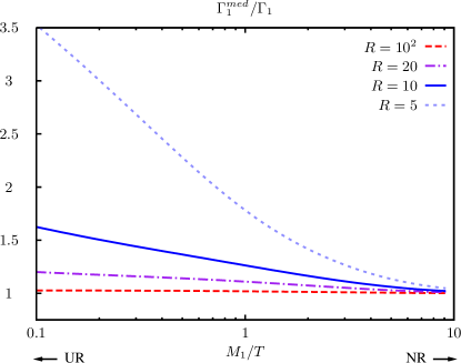
Furthermore, it strongly depends on the values of the degeneracy parameter , as can be seen in Fig. 9.
Even for reasonable values of the degeneracy parameter the effective decay width can be twice as large as in vacuum. This leads to a faster decay of the toy-Majoranas. Also the inverse decay processes are more efficient in washing out the asymmetry. In other words, the increase in the generated asymmetry due to the enhancement of the CP-violating parameter can be partially compensated by the increase of the in-medium decay widths. Let us also note that the observed enhancement of the total in-medium decay widths could be very important in the scenarios with very small values of the degeneracy parameter Boyarsky et al. (2009); Shaposhnikov (2008).
IV Numerical results
For the moment we consider numerical solutions only for the strongly hierarchical case, as the resonant case is more involved and one cannot obtain consistent Boltzmann equations for the maximal resonant case. To obtain the Boltzmann equations for and we integrate Eqs. (3) and the corresponding equation for , together with Eq. (5), over . The Boltzmann equations for are obtained from Eq. (B.5). As one can infer from Fig. 4, in the hierarchical case the off-diagonal components of the full propagators are subdominant and the diagonal components of are almost identical to those of . Therefore, we can neglect the off-diagonal components in the kinetic equations (B.5) for the full propagators and approximate them by the kinetic equations (144) for the corresponding diagonal propagators . The Boltzmann equations are then obtained after using the Kadanoff–Baym ansatz (8) and the quasiparticle approximation (9).
We solve the coupled system of Boltzmann equations in the spatially homogeneous and isotropic case in (spatially flat and radiation dominated) Friedman–Robertson–Walker space-time. They take the form
| (67) |
where is the Hubble parameter. As usual, the integrations over the time components of each of the invariant four-volume elements in the collision terms can be performed trivially after the quasiparticle approximations for the spectral functions have been inserted.
The resulting system of Boltzmann equations takes the same form as the one presented in Garny et al. (2009a) for the vertex contributions. As in the vertex case the structure differs from the usual one obtained in the conventional bottom-up approach. In particular, we do not need to include the RIS part of the collision terms for the processes because our collision terms for the processes and do not suffer from the generation of an asymmetry in equilibrium. The form of these equations is also necessary to guarantee cancellation of the gain- and loss-term contributions in equilibrium when the quantum statistical terms are present. This structure can be translated directly from the toy-model to established scenarios of leptogenesis and baryogenesis by analogy. Therefore, we consider it as important, also for phenomenological studies, and repeat it here:
| (68a) | ||||
| (68b) | ||||
| (68c) | ||||
Here, denotes the collision term for a process . The collision terms for the scattering processes in (68a) are given by
| (69a) | ||||
| (69b) | ||||
Replacing with in Eqs. (69) one obtains the analogous terms in the equation for . The collision terms in Eq. (68c) are obtained by inserting the diagonal components of the self-energy Eq. (184) into Eq. (144):
| (70) |
In the framework of the toy model the CP-violating parameter for the self-energy loop contributions given in Eq. (38), in the strongly hierarchical limit , differs by just a (symmetrization) factor from the vertex contributions. It appears explicitly in the collision terms for the (inverse) decay of into or :
| (71a) | ||||
| (71b) | ||||
The network of Boltzmann equations (68) should be understood in a generalized sense. The “amplitudes” which appear here differ from the usual perturbative matrix elements and do not share their symmetry properties.
In order to study the effect of the quantum corrections, we can again compare the results obtained by integrating the network of Boltzmann equations with quantum-corrected with the corresponding ones in the vacuum limit . The computation is started at sufficiently high temperatures so that all species, including with mass , have relativistic initial distributions. In addition, we assume that the interactions are in chemical equilibrium in the beginning, i.e. . We start with sufficiently negative chemical potentials as to avoid Bose–Einstein condensation of the different species555As was explained in Garny et al. (2009a) this necessity arises here, because we consider the system (68)-(71) as closed so that there are no interactions which can remove the produced over-densities of ’s and ’s from the system. Therefore and can in principle undergo Bose–Einstein condensation, which we avoid by choosing and appropriately. Such interactions will be present in a phenomenological scenario. Whether the possibility of Bose–Einstein condensation exists in such scenarios will have to be answered by solving appropriate kinetic equations..
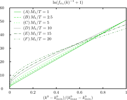
We choose the coupling (and via and ) such that the scattering rates are much larger than those of the decays and inverse decays. This assures that the light species are kept in kinetic equilibrium, as in the standard leptogenesis scenario. As shown in Garny et al. (2009a) there is no need to compute the collision integrals for scattering explicitly in this case. This means that they can be described in terms of four parameters , and , which obey the relation . Hence, we studied the evolution of and in terms of only three parameters. In contrast, the full equation for was discretized on a grid with momentum modes and solved simultaneously. For this purpose, homogeneity and isotropy was assumed, so that the angular integration can be performed as in Hohenegger (2009) in a rather general case or in the appendix of Garny et al. (2009a) for the present special case. As shown in Fig. 10, for small washout parameters,
| (72) |
the distribution function can deviate significantly from the equilibrium form (for which the curves would be straight lines). An equilibrium form would be a necessary assumption to obtain rate equations.
The generated “baryon” asymmetry is defined as
| (73) |
where and are the number densities of species and and is the standard cosmological entropy density Kolb and Turner (1990). We denote the analogous quantity, corresponding to the solution for , by .
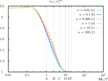
Fig. 11 shows the result for the ratio for various values of the washout parameter. Comparing it to the thermal equilibrium result in Fig. 3 one sees a flattening for small which is caused by the finite chemical potential of and in the initial conditions. One would obtain larger corrections if additional interactions for and would be introduced in order to start with smaller chemical potentials.
The generated “baryon” asymmetry does not depend monotonously on the washout parameter when the medium corrections are taken into account. This can be inferred from Fig. 12 where the dependence of the final asymmetries and are presented.
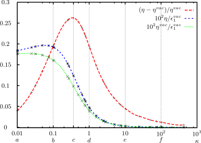
In the present case, where and are bosons, the quantum corrections always lead to an enhancement of the asymmetry compared to the results without the corrections and the asymmetry has a maximum for moderate washout factors . The maximum of the relative enhancement of about is reached at . The enhancement of due to the quantum corrections is suppressed at large washout factors, since the same processes which create and diminish the asymmetry, are effective at late times, where the CP-violating parameter takes smaller values (compare Fig. 11). In the opposite case of small , the particles decay late so that the washout is ineffective. However, the interval of integration in Eq. (35) is located at relatively large momenta since the mass increasingly dominates the relativistic energies as the momenta are red shifted to smaller values. This means that the integration is over an interval in which the distribution becomes smaller and smaller. Therefore, the relative quantum corrections go to zero for small .
This interpretation of the results was already given in Garny et al. (2009a) as they are the same for the vertex and self-energy contributions in the hierarchical limit. We can here draw the additional conclusion that the combined effect from both contributions is the same in this limit. This is important since they could in principle have opposite effects. This is not the case as the self-energy and vertex CP-violating parameters differ only by a positive prefactor, just as in the vacuum case. However, differences between the two can appear in the resonant regime. In this case the expressions for the vertex and self-energy contributions to have a different momentum dependence. Additionally, in general one has to take into account a further Boltzmann equation for the second heavy species , which is currently being studied. We would like to stress again that the size and sign of the corrections depend on the quantum statistics of the particles in the vertex- and self-energy loops and will be different in a phenomenological scenario.
V Conclusions and outlook
In this paper, we have studied leptogenesis in a simple toy model consisting of one complex and two real scalar fields in a top-down approach, using the Schwinger–Keldysh/Kadanoff–Baym formalism as starting point. This treatment, based on nonequilibrium quantum field theory techniques, is motivated by the fact that it allows a unified description of two key ingredients of leptogenesis, namely deviation from thermal equilibrium and loop-induced CP-violation.
We find that the structure of the kinetic equations automatically ensures that no asymmetry is produced in thermal equilibrium. In other words there is no need for the real intermediate state subtraction, i.e. the formalism is free of the double-counting problem typical for the canonical approach.
One of the key quantities in leptogenesis is the CP-violating parameter. Earlier studies have shown that there are two sources of CP-violation, the vertex and the self-energy contribution. In this work, we have concentrated on the latter. We have found that for scalar fields medium effects increase the self-energy contribution to the CP-violating parameter.
Contrary to the results obtained earlier in the framework of thermal field theory by replacing the zero temperature propagators with finite temperature propagators in the matrix elements of the Boltzmann equation, the medium corrections depend only linearly on the particle number densities.
Although the formal description of the self-energy and vertex contributions to the CP-violating parameter is technically quite different, the results for both are very similar qualitatively and, in the hierarchical case, even quantitatively. In this work, we additionally studied the quasidegenerate case, for which the self-energy contribution is essential.
We have shown that the canonical expression for the self-energy CP-violating parameter is only applicable in the hierarchical case, even though it does not diverge in the limit of equal masses. In the resonant regime the interactions modify the mass spectrum of the quasiparticle excitations. Furthermore, using the Kadanoff–Baym formalism, it is possible to take a resummation of resonant contributions into account. Both effects lead to changes in the expression for the CP-violating parameter. For moderate values of the degeneracy parameter the resonance corrections can enhance the CP-violating parameter by a factor of two. Therefore, it is important to take these corrections into account in numerical simulations.
Another important effect is the resonant and medium enhancement of the total decay widths. It leads to a faster decay of the heavy particles and more efficient washout of the generated asymmetry. Therefore, the increase in the generated asymmetry due to the enhancement of the CP-violating parameter can be partially compensated by the increase of the in-medium decay widths.
In the “maximal resonant” regime the Boltzmann picture is no longer applicable. This can be attributed to the fact, that in this regime the peaks of the spectral functions of the heavy (toy-)neutrino fields overlap and it is no longer possible to unambiguously define quasiparticles and one-particle distribution functions. Furthermore, the off-diagonal components of the correlation functions no longer have two pronounced peaks and therefore it is not possible to describe the mixing effects in terms of the corresponding on-shell CP-violating parameters. Consequently, in this regime the calculation of the generated asymmetry requires us to use at least two-by-two matrix equations for the diagonal and off-diagonal components of the propagators of the heavy fields with (in general) off-shell momenta. These can be obtained from the quantum kinetic equations by dropping the Poisson brackets on the right-hand side. Furthermore, since the microscopic time scales and the macroscopic time scales can be of the same order of magnitude in the maximal resonant regime, memory effects can play an important role. Taking both off-shell and memory effects into account consistently requires the use of the full system of Kadanoff–Baym equations.
The formalism developed in this paper also provides a powerful tool for analyzing quantum nonequilibrium effects induced by the expansion of the early Universe. In particular, there is a small additional “spontaneous” contribution to the CP-violation in the system similar to that encountered in electroweak baryogenesis Konstandin et al. (2005); Prokopec et al. (2004a, b); Konstandin et al. (2006) This effect will be investigated in a forthcoming paper Garny et al. (2009b).
Acknowledgements
This work was supported by the “Sonderforschungsbereich” TR27 and by the “cluster of excellence Origin and Structure of the Universe”. We would like to thank J. Berges, J-S. Gagnon, A. Ibarra and M. M. Müller for helpful comments and discussions.
Appendix A CP-violating parameter
In this appendix, we review the calculation of the self-energy contribution to the CP-violating parameter in vacuum, , in the conventional in-out formalism.
Since the toy-Majoranas are unstable, they cannot appear as in- or out-states of S-matrix elements. Instead, their properties are defined by S-matrix elements for scattering of stable particles mediated by the unstable neutrino Veltman (1963). Resumming the propagator of the intermediate heavy state, we can separate two-body scattering processes in resonance contributions and the rest. The CP-violating part of the resonance contribution can then be interpreted as a characteristic of the on-shell intermediate toy-Majorana Pilaftsis (1997); Plümacher (1998).
The amplitude of the -channel two-body scattering process (see Fig. 13) can conveniently be expressed as
| (74) |
where and represent the vertices and that include the wave functions of the initial and final states, and are the full propagators obtained by resumming an infinite series of toy-Majorana self-energy graphs Pilaftsis (1997).
The resummation can be performed using the Schwinger-Dyson equation in vacuum:
| (75) |
At one-loop level the self-energy reads
| (76) |
where
| (77) |
and contains the divergent contribution. To renormalize the mass and the self-energy we introduce the wave-function and mass counterterms to the Lagrangian:
| (78) |
where and are symmetric two-by-two matrices. This implies that the renormalized self-energy is given by
| (79) |
In the on-shell renormalization scheme the dispersive parts of the components of the renormalized self-energy must satisfy the conditions
| (80a) | ||||
| (80b) | ||||
Using (79) and (80) and the explicit form of the bare self-energy we calculate and . Substituting them into (79) we find
| (81a) | ||||
| (81b) | ||||
Inverting (75) we obtain for the components of the renormalized resummed propagator:
| (82a) | ||||
| (82b) | ||||
Because of the presence of absorptive terms in (81) the determinant of the inverse propagator in (82) has two poles in the complex plane at
| (83) |
where is the tree-level decay width of . Expanding (82) around the poles and substituting the leading expansion terms to (74) we find Pilaftsis and Underwood (2004)
| (84) |
where
| (85) |
The modulo squared of the scattering amplitude is then given by
| (86) |
The Breit-Wigner propagators in the diagonal terms of (A) strongly peak on the mass shell of the quasiparticles, i.e. at and rapidly decrease off the mass shell. In the limit of vanishing decay widths
| (87) |
Furthermore, if then the two Breit-Wigner propagators do not overlap and we can neglect the cross terms in (A). In other words, in this approximation the resonant (real intermediate state) part of the amplitude is given by
| (88) |
Equation (88) suggests, that should also be evaluated at . As follows from (A) to leading order in the couplings its modulo squared can be represented in the form
| (89) |
Using the explicit form of the renormalized self-energy (81) we obtain for the CP-violating parameters in vacuum:
| (90) |
Because of the presence of the term in the denominator of (90), it does not diverge if . However, the condition is not satisfied in this case and therefore the approximations we have made to derive (90) are not valid in this limit. Let us also note that due to approximation (87) the CP-violating parameter (90) characterizes on-shell heavy particles.
Integrals of the left- and right-hand sides of (87) over are equal only if we integrate in the range from to . But in the channel the momentum transfer squared is always positive. Moreover, the functions also depend on . Thus, in the transition from (A) to (88), i.e. in replacing the Breit-Wigner propagator by a Dirac -function and evaluating at we have made an approximation which, strictly speaking, is only valid in the limit . We could perform the integration more carefully and take the finite widths into account using Cauchy’s integral theorem and evaluating at the poles . This leads to a slightly different expression for the CP-violating parameter Anisimov et al. (2006):
| (91) |
Equation (91) can be considered as a better estimate of the CP-violating effects in the system. However, since the on-shell approximation (87) no longer applies, one can not interpret (91) as an expression for the CP-violating parameter of an on-shell state. In other words, strictly speaking, (91) would require us to use an off-shell generalization of the Boltzmann equation.
Let us also note that in the case , which we have considered here, the difference between the two expressions for the CP-violating parameter can be neglected.
Appendix B Mixing real scalar fields
In this appendix, we derive the Kadanoff–Baym, quantum kinetic and Boltzmann equations for a system of two (or, in general, ) mixing real scalar fields.
B.1 Schwinger–Dyson equation
The generating functional of such a system reads
| (92) |
The bilinear external source is a -by- matrix with the property , where in the toy-model. Note that the field and the external sources are defined on the positive and negative branches of a closed real-time contour; see Fig. 14. Throughout this work, we use the compact notation of Ref. Danielewicz (1984a), which avoids the doubling of the degrees of freedom. In particular, note that the indices refer to the two real scalar fields in the toy model.

The functional derivatives of the generating functional for connected Green’s functions, , with respect to the external sources read
| (93a) | ||||
| (93b) | ||||
where is the expectation value of the field operator. The propagator is a –by– matrix; its off-diagonal components describe the mixing of the two fields. We emphasize again that the indices refer to the field content, and have nothing to do with the branches of the time-contour.
Performing a Legendre transform of the generating functional for connected Green’s functions, we obtain the effective action
| (94) |
Its functional derivatives with respect to the expectation value and the propagator reproduce the external sources:
| (95a) | ||||
| (95b) | ||||
where and is the determinant of the space-time metric.
Shifting the fields by their expectation values , we can rewrite the effective action in the form
| (96) |
Next, we tentatively write the effective action in the form
| (97) |
which defines the functional .
Differentiation of the third term on the right-hand side with respect to the field propagators yields the inverse free propagators. Note that the latter one is diagonal – in the absence of interactions the two fields do not mix:
| (98) |
where is a generalized Dirac -function.
The second term on the right-hand side is defined by the path integral
To calculate the functional derivative of , we take into account that
| (99) |
After some algebra and use of (99), we obtain
| (100) |
The functional derivative of (97) with respect to then reads
| (101) |
The considered physical situation corresponds to vanishing sources. Introducing the self-energy,
| (102) |
we can then rewrite (B.1) in the form
| (103) |
As can be inferred from (103), off-diagonal components of are induced by off-diagonal components of . In the considered model they arise because both real scalars couple to the “baryons”.
B.2 Kadanoff–Baym equations
The statistical propagators and spectral functions are defined by
| (105a) | ||||
| (105b) | ||||
From the definitions (105) it follows that
| (106) |
The time-ordered Schwinger–Keldysh propagator (which is the analogue of the Feynman propagator on the closed time path) is a linear combination of these functions:
| (107) |
Upon use of the signum- and -function differentiation rules, the action of the operator on the second term in (107) yields a product of and . Using the definition (105) and the canonical commutation relations Isham (1978)
| (108) |
where , we find for the derivative of the spectral function
| (109) |
Multiplication of (109) by then gives the generalized Dirac -function , which cancels the -function on the right-hand side of (B.2). Furthermore, we decompose the self-energy according to
| (110) |
The resulting system of Kadanoff–Baym equations reads (see Berges (2004a); Hohenegger et al. (2008b) for more details):
| (111a) | ||||
| (111b) | ||||
In the limit of just one scalar field it reverts to the system derived in Hohenegger et al. (2008a). Numerical solutions of full Kadanoff–Baym equations, for systems involving effectively a single degree of freedom in the scalar sector, have been studied e.g. in Danielewicz (1984b); Berges and Cox (2001); Berges (2002); Aarts and Berges (2002); Berges et al. (2003); Juchem et al. (2004); Arrizabalaga et al. (2005); Lindner and Müller (2006, 2008).
B.3 Quantum kinetics
The system of Kadanoff–Baym equations can be rewritten in terms of the advanced and retarded propagators, and :
| (112) |
In order to close the system, Eqs. (B.3) must be supplemented with the analogous equations for the retarded and advanced propagators:
| (113) |
From the definitions of the retarded and advanced propagators and relations (106) one can infer that
| (114) |
Therefore, after interchanging and and then and in (B.3), we obtain
| (115) |
The same operation applied to (B.3) yields
| (116) |
Following the usual procedure, we introduce the center and relative coordinates and Winter (1985). The Wigner transform of the statistical propagator is defined by
| (117) |
The definition of the Wigner transform of differs from (117) by an overall factor of . From (106) it then follows that
| (118) |
where the hats denote the corresponding matrices and the superscript ‘T’ denotes transposition. As we see, the Wigner transforms are Hermitian matrices. The Wigner transforms of the retarded and advanced propagators are defined analogously to (117). Using (B.3) one can then show that
| (119) |
Just as in the case of a single real scalar field Hohenegger et al. (2008a), from the definitions of the Wigner transforms, relation (B.3) and the equality it follows that
| (120) |
We could have derived Eqs. (119) and (120) using the spectral representation of the retarded and advanced propagators
| (121) |
The spectral representation also implies that and can be represented as a linear combination of two Hermitian matrices:
| (122) |
Let us now subtract (B.3) from (B.3) and Wigner transform the left- and the right-hand sides of the resulting equation. On the right-hand side we neglect the memory effects, that is, we discard the function and replace by . Furthermore, we keep only terms at most linear in the Wigner transform of the covariant derivative ; see Hohenegger et al. (2008a) for more details. Introducing
the Poisson brackets,
| (123) |
the generalized Poisson brackets666If the matrices and are hermitian and commute, then .
| (124) | ||||
and
| (125) |
we can rewrite the result in a compact form:
| (126) |
In the case of a single scalar field the commutator in (124) vanishes and, using (122), we can then show that the quantum kinetic equation (B.3) for the spectral function and statistical propagator revert to those derived in Hohenegger et al. (2008a). After some algebra we rewrite the quantum kinetic equation for the spectral function in the form:
| (127) |
where
| (128) |
The quantum kinetic equations must be supplemented by the corresponding constraint equations. To derive these, we add up the Wigner-transforms of (B.3) and (B.3). To linear order in the gradients the resulting constraint equations read
| (129) |
where we have introduced and to shorten the notation. In the case of a single scalar field (B.3) revert to those derived in Hohenegger et al. (2008a). After some algebra we can again simplify the constraint equation for the spectral function:
| (130) |
To close the system of the constraint equations (B.3) we have to derive the constraint equation for the function or, alternatively, for the retarded propagator:
| (131) |
where the operation is defined as the operation but does not involve Hermitian conjugation. Unlike in the case of a single scalar field, the constraint equations (B.3) and (B.3) are not algebraic and cannot be solved easily. The solution of the algebraic part of (B.3) and (B.3) is not a solution of the complete differential equations. Therefore, we conclude that even to linear order in the gradients the spectrum of the mixing scalar fields depends on the derivative terms described by the Poisson brackets.
B.4 Solution in the equilibrium limit
Since in vacuum and in thermal equilibrium the system is homogeneous, isotropic and static the two-point functions are translationally invariant, i.e. do not depend on the center coordinate . Therefore, in thermal equilibrium and in vacuum, the Poisson brackets (B.3) vanish. In the following, we discuss the solutions of the constraint equations obtained by neglecting the Poisson brackets. However, we do not make use of any relations relying on periodic equilibrium boundary conditions. Therefore, the formal solutions should also be a reasonable approximation sufficiently close to equilibrium, when gradient contributions are small. In this case, (B.3) reduces to an algebraic matrix equation. Its solution reads
| (132) |
From the definition (125), relation (119) and the analogous relations for the retarded and advanced self-energies it then follows that
| (133) |
From relation (122) it follows that
| (134) |
Using (132) and (133) we then find that in equilibrium and in vacuum
| (135) |
Similarly to (B.4), the equilibrium (or vacuum) solution of the constraint equation for the statistical propagator is given by
| (136) |
Note that unlike in (B.4) the order of the retarded and advanced components is no longer arbitrary. Let us now split into off-diagonal and diagonal matrices, the latter being denoted by . Next we
define diagonal matrices
| (137) |
and
| (138) |
where denotes the diagonal components of the self-energy matrices . Explicitly
| (139) |
In the quasiparticle approximation, i.e. in the limit of vanishing self-energy, the diagonal spectral function (139) reverts to (9). From (137) we also obtain
| (140) |
In the quasiparticle approximation it reduces to (37). Combining (B.4) and (136) with (137) and (138) we can express the full propagators in terms of the diagonal ones:
| (141) |
where is the off-diagonal part of . From (18) and the definitions of the Wigner-transforms of the statistical propagator and spectral function it follows that the corresponding Wightman propagators are given by
| (142) |
Inverting the resulting (two-by-two) matrices and taking into account that the products of and are off-diagonal we arrive at (22).
B.5 Boltzmann equation
To obtain Boltzmann equations we neglect the (conventional) Poisson brackets on the right-hand side of (B.3). In the Boltzmann approximation the field’s mass disappears in the difference of the diagonal components. However, the difference of the masses squared, , appears in the equations for the off-diagonal terms. Moving these terms to the right-hand side we find
| (143) |
where all the functions are evaluated at the same point of the phase-space. Substituting the equilibrium solutions (B.4) and (136) into (B.5) we see that its right-hand side vanishes indeed.
If all the matrices in (B.5) were diagonal, it would revert to two independent systems of Boltzmann equations for the statistical propagator and spectral function:
| (144a) | ||||
| (144b) | ||||
Equation (144b) is consistent with the fact, that for a single scalar field the solution for the spectral function (139) is valid up to the first order in the gradients. This allows us to employ the Kadanoff–Baym ansatz for the statistical propagator, , and rewrite the original system of the Boltzmann equations (144) as a Boltzmann equation for the distribution function . In the case of two mixing scalar fields the situation is quite different. The solution (B.4) is valid only in equilibrium. As follows from (B.3), out of equilibrium the off-diagonal components of the spectral function receive corrections linear in the gradients. Strictly speaking, this means that we can not introduce a generalized Kadanoff–Baym ansatz and reduce (B.5) to a system of two equations for the one-particle distribution functions. In general, to analyze the generation of the asymmetry, one has to solve the system of the Boltzmann equations (B.5) for the full spectral function and statistical propagator. Only when the off-diagonal components are subdominant (which is the case in the hierarchical and resonant regime, but not in the maximal resonant limit) one can approximate (B.5) by (144). The Boltzmann equations for the diagonal propagators (144) do not contain the self-energy CP-violating parameter. Given that the contributions proportional to the vertex CP-violating parameter also cancel out in the Boltzmann equations for the real scalars Garny et al. (2009a), this is an expected property.
Appendix C Integration over the contour
In this appendix we calculate two integrals over the closed-time-path contour, shown in Fig. 14, which are required for the derivation of the self-energy contribution to the CP-violating parameter in the Kadanoff–Baym formalism. Let us first consider the integral
| (145) |
Assuming that the two-point functions possess a decomposition into statistical and spectral components similar to Eq. (107), we find
| (146) |
These formulas are required to obtain the right-hand side of (111). Replacing and by and we can rewrite the right-hand side of (C) as an integral over the whole axis. From (C) it also follows, that
| (147) |
Next we consider the integral
| (148) |
Since can be represented as an integral of a product of and over the contour, its spectral and statistical components are given by (C) with replaced by . Furthermore, using (147) we find
| (149) |
Building the linear combinations of the spectral and statistical components we can easily derive the components from (C).
We will now calculate the Wigner-transform of (C) in the Boltzmann approximation. That is, in each of the functions in (C) we neglect the deviation of the corresponding center coordinate from . For instance:
| (150) |
In this approximation the integration over and induces a simple relation between the momenta . Integration over the relative coordinate induces an additional constraint . Therefore we obtain:
| (151) |
This completes the calculation of the Winger transform.
Appendix D Renormalization
In this appendix, we derive the renormalization prescription (43) employed in Sec. III for the derivation of the CP-violating parameter in the resonant case. For the level of approximation considered there, it is sufficient to include perturbative one-loop mass and field counterterms (see Appendix A)777The renormalization of the full Kadanoff–Baym equations (111) has been discussed in refs. Borsanyi and Reinosa (2008); Garny and Müller (2009), see also van Hees and Knoll (2002a, b); Blaizot et al. (2004); Berges et al. (2005a, b). for the real scalar field ,
| (152) |
Including the counterterms in the Lagrangian (I) results in a modification of the Schwinger-Dyson equation (12),
| (153) |
(using matrix notation; see Appendix B.1), where
Proceeding analogously as in Sec. III, we decompose the renormalized self-energy into diagonal and off-diagonal parts,
and define a renormalized “diagonal” propagator by
| (154) |
In analogy to the steps leading to Eq. (III), we find for the full Wightman functions
where and denote the off-diagonal parts of and , respectively. Using this, we find that the renormalized version of Eq. (22) can be obtained by replacing , as well as . The latter prescription coincides with Eq. (43) for .
The diagonal part of the self-energy enters in the renormalized diagonal propagator ; see Eq. (154). Since this equation can be split into independent equations for each entry on the diagonal, it is analogous to the case of a single real scalar field; see e.g. Hohenegger et al. (2008a). The solution of the corresponding Wigner-transformed kinetic equations for the retarded and advanced propagator reads (up to second-order gradients; see also Eq. (137)),
| (156) |
where the renormalized self-energies are determined in accordance with Eq. (43) for . Since , the spectral function also contains renormalized self-energies. Furthermore, using the Kadanoff–Baym ansatz implies that also the statistical propagator, and therefore also the Wightman functions, are finite.
Thus, altogether, we find that the prescription (43) renormalizes the diagonal as well as off-diagonal components of the relevant propagators.
Appendix E Analysis in the full KB formalism
In this appendix, we derive a time-evolution equation for the “baryon” asymmetry within nonequilibrium field theory. It is based on the approximate -symmetry of the toy-model Lagrangian (I), and does not require any further approximations beyond the 2PI truncation. As we will see, in the Boltzmann limit, the resulting equation for the asymmetry coincides with those obtained from the quantum-corrected Boltzmann equations discussed above.
The Lagrangian (I) can be split into -conserving and -violating parts,
where
| (157) | ||||
| (158) |
The corresponding Noether current is given by
Its expectation value can be written as (note that we are working in the Heisenberg picture)
where is the statistical propagator of the complex -field.
Because of the presence of , the Noether current is in general not conserved. Its divergence reads
| (159) |
The expression in the last line can be evaluated by using the Kadanoff–Baym equations for the complex scalar field. These can be derived analogously to the system (111) of Kadanoff–Baym equations for the real scalar fields. They read
| (160a) | ||||
| (160b) | ||||
We use the notations of Ref. Garny et al. (2009a) here. In particular, the statistical propagator and the spectral function of the complex field are defined analogously to Eq. (105). The upper equations possess an equivalent representation in terms of the antiparticle propagators
| (161) |
and antiparticle self-energies (defined analogously). The Kadanoff–Baym equations for the antiparticles then take the same form as Eqs. (160), except for the replacement and .
The Kadanoff–Baym equations for and can now be used to evaluate the right-hand side of Eq. (E),
| (162) | |||||
By using the retarded and advanced propagators
| (163) |
as well as analogous definitions for the antiparticle propagators, we finally find the following equation of motion for the toy-baryon current:
So far, the derivation is quite general and the upper equations are formally fulfilled even in the exact theory. To obtain a closed system we have to express the self-energies in terms of the two-point functions. In the Kadanoff–Baym formalism the self-energies are obtained by functional differentiation of the 2PI effective action. Approximations can be obtained by truncating the 2PI functional, for example at a certain loop order. This leads to so-called -derivable approximations, which are conserving, i.e. they automatically respect the conservation laws of the full theory Ivanov et al. (1999); Knoll et al. (2001). This means that, in the limit of vanishing -violation, the baryon current obtained in the Kadanoff–Baym formalism is indeed conserved at any loop order of the 2PI functional.
The structure of the 2PI effective action in two-loop approximation can be read off the diagram in Fig. 2 (a):
| (165) |
Differentiating the effective action with respect to the two-point function of the complex scalar field we obtain
| (166) |
The statistical and spectral components of the self-energy are given by
| (167a) | ||||
| (167b) | ||||
The upper expressions, together with the Kadanoff–Baym equations (160), as well as the corresponding equations for the toy-Majorana fields (111) and (13), form a closed system of equations. Inserting their solutions into Eq. (E) yields the time-evolution of the toy-baryon asymmetry
| (168) |
Equation (E) takes memory and quantum off-shell effects into account in a very general way, and is valid even very far from thermal equilibrium. Furthermore, due to the self-consistency it implicitly resums a large number of multiparticle scattering processes. However, this feature also makes the (numerical) solution of the full equations difficult. In a typical leptogenesis scenario one is interested in a situation where the deviations from equilibrium are comparably mild. In this case, it is possible to obtain simplified evolution equations for the asymmetry from Eq. (E). In the following, we will show that the resulting equations are equivalent to those obtained from the kinetic evolution equations of the particle distribution function, provided both are based on the identical truncation of the 2PI effective action.
E.1 Consistency with the kinetic approach
Usually, within the kinetic approach, the baryon asymmetry is calculated by evaluating the difference of particle and antiparticle distribution functions,
| (169) |
where and are obtained from Boltzmann-like kinetic equations. Equations (168,E) for the toy-baryon asymmetry discussed above provide a complementary possibility to calculate the asymmetry. In this context, the question arises, under which conditions both approaches are equivalent. In the following, we will show that equivalence holds provided (i) one uses the top-down or quantum-corrected kinetic equations, which are obtained from the gradient expansion of the full Kadanoff–Baym equations, (ii) the evolution equation (E) of the baryon current is expanded to the same order in the gradient expansion, and (iii) both sets of equations are based on the same truncation of the 2PI effective action. This can be seen as follows: By performing a Wigner transformation and a first-order gradient expansion of Eq. (E), and using relations (E), we obtain on the one hand
| (170) | |||||
where the curly brackets denote the usual Poisson brackets, and we have used the decomposition .
On the other hand, the quantum kinetic equation for obtained from a first-order gradient expansion of the Kadanoff–Baym equation (160) reads (see e.g. Ref. Garny et al. (2009a))
| (171) | |||||
where . Inserting this equation into Eq. (170) yields
| (172) |
Using , we can write this as
| (173) |
Inserting the Kadanoff–Baym ansatz yields
| (174) |
where we have assumed a symmetric spectrum, . For a spatially homogeneous system, the frequency integration yields the particle distribution function of the momentum mode at time ,
Thus, using Eq. (168), we find
| (175) | |||||
Thus, we find that the baryon asymmetry inferred from the equation of motion of the baryon current coincides with the asymmetry obtained from the corresponding kinetic approach, under the conditions discussed above (this is in accordance with the general analysis of Ref. Knoll et al. (2001)).
E.2 Self-energy contribution
Here, we briefly want to discuss the time-evolution of the baryon asymmetry within the 2PI two-loop truncation based on the full evolution equation (E). As discussed in Sec. II, the 2PI two-loop approximation captures the self-energy contribution to the CP-violating decays and inverse decays, whereas the vertex contribution requires to take also three-loop diagrams in the 2PI functional into account Garny et al. (2009a). Thus, the 2PI two-loop case provides a possibility to investigate whether an asymmetry can be induced by the self-energy-type contributions. The latter question has, after some controversial discussions, been answered e.g. in Ref. Roulet et al. (1998) within the Boltzmann framework. In the following, we address the same question, from a slightly different point of view, within nonequilibrium quantum field theory.
Assuming spatial homogeneity, we can write the total baryon asymmetry as
| (176) |
From Eq. (E), we obtain the following evolution equation for the baryon asymmetry in momentum mode :
where .
By inserting the 2PI two-loop expressions (167) into the upper equation, and using Eq. (106), we obtain
| (178) | |||||
where all propagators are evaluated at . In the limit of vanishing CP-violation, i.e. for , the Eq. (178) possesses a baryon-symmetric solution for which , (see Appendix F), and at all times. For an initial state which is asymmetric, the terms proportional to tend to wash out the asymmetry and would, in flat space-time, asymptotically drive .
Here, we are interested in the opposite situation. This means, we want to answer the question whether can deviate from zero at some instant of time although it vanishes initially, . Any change of with time requires, of course, nonzero B-violation (i.e. ), since would correspond to a conserved charge otherwise. Additionally, from Eq. (178), we see that the generation of an asymmetry also requires , i.e. nonvanishing CP-violation. Finally, a deviation from thermal equilibrium is required, since otherwise time-translation invariance would require to be equal to its initial value at all times. Thus, the quantum evolution equation (178) obtained from the 2PI two-loop approximation is in accordance with the Sakharov conditions. In general, we therefore expect that can deviate from for some , if and if the system deviates from equilibrium888There are two potential sources for deviations from thermal equilibrium, namely the space-time expansion as well as the initial conditions. In order to check whether Eq. (178) can indeed describe the generation of an asymmetry, we concentrate on the latter source for simplicity. We note that, in order to describe equilibrium initial conditions of the full quantum evolution equations, it would be necessary to include non-Gaussian correlations of the initial state (see e.g. Garny and Müller (2009)). However, since the latter play no role in the kinetic approach (the initial time is formally sent to the infinite past when performing a Wigner transformation), we do not consider them here. . In order to make this statement more quantitative, we consider a Taylor expansion of Eq. (178) around the initial time . The first nonvanishing contribution turns out to be of order four,
Thus, for a symmetric initial state with , an asymmetry can arise if , as expected, and if . The latter condition is, however, not necessary. If and , the leading term reads
Consequently, the full quantum evolution equations support the observation that an asymmetry can be generated from self-energy-type contributions to the CP-violating decays.
Appendix F Baryonically symmetric configuration
The Wightman propagators of the complex scalar field are defined by Garny et al. (2009a)
| (180a) | ||||
| (180b) | ||||
Applying the operator of charge conjugation to (180) we obtain
| (181a) | ||||
| (181b) | ||||
where the superscript ‘c’ denotes the charge-conjugated quantities. In a baryonically symmetric configuration . Therefore in this case . In turn, for the statistical propagator and spectral function this implies
| (182) |
Since the full propagator is related to and by
| (183) |
we conclude that in a baryonically symmetric configuration .
Differentiating the effective action with respect to the two-point function of the real scalar fields we obtain the two-loop contribution to the self-energy:
| (184) |
In the symmetric configuration it takes the form
| (185) |
i.e. this matrix is symmetric. This is also true for the spectral, statistical, retarded and advanced self-energies that can be derived from (185).
Appendix G One-loop integral
Here we calculate the one-loop self-energy integrals given in Eq. (III.1),
| (186) |
evaluated for an on-shell momentum where . We have omitted the superscript ‘s’ here since the calculation applies also to baryonically asymmetric states. We first consider . Inserting the quasiparticle approximation for the complex field, see Eq. (7), and the Kadanoff–Baym ansatz , one finds
| (187) |
where we have used a manifestly Lorentz-covariant notation. In the rest-frame of the medium . Note that only the poles with and contribute since . The integration over is trivial due to the Dirac- in the first line. In order to perform the remaining integrations, we express the integrand in the rest-frame of the decaying “heavy neutrino”, for which and ,
| (188) |
where and . The Dirac -function requires . Using furthermore , we find
| (189) |
where . After integrating over , one obtains
| (190) |
If the medium is approximately symmetric, , we can write the result in the form presented in Eq. (34).
Let us now turn to . As above, we insert the Kadanoff–Baym ansatz for and use the quasiparticle approximation for , yielding
| (191) | ||||
In the quasiparticle limit, one can express in the form
| (192) |
where denotes the principal value. As above, we evaluate the integral in the rest-frame of the decaying particle. The result of the calculation reads
| (193) |
The vacuum contribution, which corresponds to the limit , depends only on due to Lorentz invariance of the vacuum state. It is logarithmically divergent. However, after renormalization, only the difference appears, which is finite. For the on-shell momentum considered here, we obtain
| (194) |
where . For an approximately symmetric state, the medium contribution can be written as
| (195) |
where in the limit . By introducing spherical coordinates and substituting for , we obtain
| (196) |
After performing the angular integration (and replacing ), we obtain the result stated in Eq. (III.2).
References
- Fukugita and Yanagida (1986) M. Fukugita and T. Yanagida, Phys. Lett. B 174, 45 (1986).
- Garny et al. (2009a) M. Garny, A. Hohenegger, A. Kartavtsev, and M. Lindner, Phys. Rev. D80, 125027 (2009a), eprint 0909.1559.
- Flanz et al. (1995) M. Flanz, E. A. Paschos, and U. Sarkar, Phys. Lett. B 345, 248 (1995), erratum-ibid.B382:447,1996, eprint hep-ph/9411366.
- Covi et al. (1996) L. Covi, E. Roulet, and F. Vissani, Phys. Lett. B 384, 169 (1996), eprint hep-ph/9605319.
- Pilaftsis (1997) A. Pilaftsis, Phys. Rev. D 56, 5431 (1997).
- Pilaftsis and Underwood (2004) A. Pilaftsis and T. E. J. Underwood, Nucl. Phys. B 692, 303 (2004), eprint hep-ph/0309342.
- Pilaftsis and Underwood (2005) A. Pilaftsis and T. E. J. Underwood, Phys. Rev. D 72, 113001 (2005), eprint hep-ph/0506107.
- Blanchet et al. (2009) S. Blanchet, Z. Chacko, S. S. Granor, and R. N. Mohapatra (2009), eprint 0904.2174.
- Kadanoff and Baym (1962) L. P. Kadanoff and G. Baym, Quantum Statistical Mechanics (Benjamin, New York, 1962).
- Covi et al. (1998) L. Covi, N. Rius, E. Roulet, and F. Vissani, Phys. Rev. D 57, 93 (1998), eprint hep-ph/9704366.
- Buchmüller and Fredenhagen (2000) W. Buchmüller and S. Fredenhagen, Phys. Lett. B 483, 217 (2000), eprint hep-ph/0004145.
- Giudice et al. (2004) G. F. Giudice, A. Notari, M. Raidal, A. Riotto, and A. Strumia, Nucl. Phys. B 685, 89 (2004), eprint hep-ph/0310123.
- Lindner and Müller (2006) M. Lindner and M. M. Müller, Phys. Rev. D 73, 125002 (2006), eprint hep-ph/0512147.
- Lindner and Müller (2008) M. Lindner and M. M. Müller, Phys. Rev. D 77, 025027 (2008), eprint 0710.2917.
- De Simone and Riotto (2007a) A. De Simone and A. Riotto, JCAP 0708, 002 (2007a), eprint hep-ph/0703175.
- De Simone and Riotto (2007b) A. De Simone and A. Riotto, JCAP 0708, 013 (2007b), eprint 0705.2183.
- De Simone (2008) A. De Simone (2008), eprint 0805.2354.
- Tranberg (2008) A. Tranberg, JHEP 11, 037 (2008), eprint 0806.3158.
- Hohenegger et al. (2008a) A. Hohenegger, A. Kartavtsev, and M. Lindner, Phys. Rev. D 78, 085027 (2008a), eprint 0807.4551.
- Anisimov et al. (2009) A. Anisimov, W. Buchmüller, M. Drewes, and S. Mendizabal, Annals Phys. 324, 1234 (2009), eprint 0812.1934.
- Gagnon (2009) J.-S. Gagnon, Nucl. Phys. A 820, 199c (2009).
- Kiessig and Plümacher (2009) C. P. Kiessig and M. Plümacher (2009), eprint 0910.4872.
- Sakharov (1967) A. D. Sakharov, JETP Letters 5, 24 (1967).
- Anisimov et al. (2006) A. Anisimov, A. Broncano, and M. Plümacher, Nucl. Phys. B737, 176 (2006), eprint hep-ph/0511248.
- Kolb and Turner (1990) E. W. Kolb and M. S. Turner, The Early universe (1990), Redwood City, CA: Addison-Wesley 547 p. (Frontiers in physics, 69).
- Schwinger (1961) J. S. Schwinger, J. Math. Phys. 2, 407 (1961).
- Keldysh (1964) L. V. Keldysh, Zh. Eksp. Teor. Fiz. 47, 1515 (1964).
- Bakshi and Mahanthappa (1963) P. M. Bakshi and K. T. Mahanthappa, Journal of Mathematical Physics 4, 1 (1963).
- Danielewicz (1984a) P. Danielewicz, Annals Phys. 152, 239 (1984a).
- Chou et al. (1985) K. Chou, Z. Su, B. Hao, and L. Yu, Phys. Rept. 118, 1 (1985).
- Calzetta and Hu (1988) E. Calzetta and B. L. Hu, Phys. Rev. D 37, 2878 (1988).
- Ivanov et al. (2000) Y. B. Ivanov, J. Knoll, and D. N. Voskresensky, Nucl. Phys. A 672, 313 (2000), eprint nucl-th/9905028.
- Knoll et al. (2001) J. Knoll, Y. B. Ivanov, and D. N. Voskresensky, Annals Phys. 293, 126 (2001), eprint nucl-th/0102044.
- Blaizot and Iancu (2002) J.-P. Blaizot and E. Iancu, Phys. Rept. 359, 355 (2002), eprint hep-ph/0101103.
- Berges and Müller (2002) J. Berges and M. M. Müller (2002), eprint hep-ph/0209026.
- Berges and Borsanyi (2006) J. Berges and S. Borsanyi, Phys. Rev. D 74, 045022 (2006), eprint hep-ph/0512155.
- Weinstock (2006) S. Weinstock, Phys. Rev. D 73, 025005 (2006), eprint hep-ph/0510417.
- Carrington and Mrowczynski (2005) M. E. Carrington and S. Mrowczynski, Phys. Rev. D 71, 065007 (2005), eprint hep-ph/0406097.
- Fillion-Gourdeau et al. (2006) F. Fillion-Gourdeau, J.-S. Gagnon, and S. Jeon, Phys. Rev. D 74, 025010 (2006), eprint hep-ph/0603212.
- Berges (2004a) J. Berges, AIP Conf. Proc. 739, 3 (2004a), eprint hep-ph/0409233.
- Berges (2004b) J. Berges, Phys. Rev. D 70, 105010 (2004b), eprint hep-ph/0401172.
- Cornwall et al. (1974) J. M. Cornwall, R. Jackiw, and E. Tomboulis, Phys. Rev. D 10, 2428 (1974).
- Špička and Lipavský (1995) V. Špička and P. Lipavský, Phys. Rev. B 52, 14615 (1995).
- Köhler (1992) H. S. Köhler, Phys. Rev. C 46, 1687 (1992).
- Köhler and Malfliet (1993) H. S. Köhler and R. Malfliet, Phys. Rev. C 48, 1034 (1993).
- Köhler and Morawetz (2001) H. S. Köhler and K. Morawetz, Phys. Rev. C 64, 024613 (2001).
- Morozov and Röpke (2006a) V. G. Morozov and G. Röpke, Cond. mat. Phys. 9, 473 (2006a).
- Morozov and Röpke (2006b) V. G. Morozov and G. Röpke, Journal of Physics: Conference Series 35, 110 (2006b).
- Davidson and Ibarra (2002) S. Davidson and A. Ibarra, Phys. Lett. B 535, 25 (2002), eprint hep-ph/0202239.
- Giudice et al. (2008) G. F. Giudice, L. Mether, A. Riotto, and F. Riva, Phys. Lett. B 664, 21 (2008), eprint 0804.0166.
- Blanchet et al. (2008) S. Blanchet, Z. Chacko, and R. N. Mohapatra (2008), eprint 0812.3837.
- Dar et al. (2006) S. Dar, Q. Shafi, and A. Sil, Phys. Lett. B 632, 517 (2006), eprint hep-ph/0508037.
- Frere et al. (2009) J.-M. Frere, T. Hambye, and G. Vertongen, JHEP 01, 051 (2009), eprint 0806.0841.
- Boyarsky et al. (2009) A. Boyarsky, O. Ruchayskiy, and M. Shaposhnikov, Ann. Rev. Nucl. Part. Sci. 59, 191 (2009), eprint 0901.0011.
- Shaposhnikov (2008) M. Shaposhnikov, JHEP 08, 008 (2008), eprint 0804.4542.
- Hohenegger (2009) A. Hohenegger, Phys. Rev. D 79, 063502 (2009), eprint 0806.3098.
- Konstandin et al. (2005) T. Konstandin, T. Prokopec, and M. G. Schmidt, Nucl. Phys. B 716, 373 (2005), eprint hep-ph/0410135.
- Prokopec et al. (2004a) T. Prokopec, M. G. Schmidt, and S. Weinstock, Ann. Phys. 314, 267 (2004a), eprint hep-ph/0406140.
- Prokopec et al. (2004b) T. Prokopec, M. G. Schmidt, and S. Weinstock, Ann. Phys. 314, 208 (2004b), eprint hep-ph/0312110.
- Konstandin et al. (2006) T. Konstandin, T. Prokopec, M. G. Schmidt, and M. Seco, Nucl. Phys. B 738, 1 (2006), eprint hep-ph/0505103.
- Garny et al. (2009b) M. Garny, A. Hohenegger, A. Kartavtsev, and M. Lindner (2009b), eprint to appear.
- Veltman (1963) M. J. G. Veltman, Physica 29, 186 (1963).
- Plümacher (1998) M. Plümacher, Nucl. Phys. B530, 207 (1998), eprint hep-ph/9704231.
- Isham (1978) C. J. Isham, Proceedings of the Royal Society of London. Series A, Mathematical and Physical Sciences 362, 383 (1978).
- Hohenegger et al. (2008b) A. Hohenegger, A. Kartavtsev, and M. Lindner, Phys. Rev. D78, 085027 (2008b), eprint 0807.4551.
- Danielewicz (1984b) P. Danielewicz, Annals Phys. 152, 305 (1984b).
- Berges and Cox (2001) J. Berges and J. Cox, Phys. Lett. B 517, 369 (2001), eprint hep-ph/0006160.
- Berges (2002) J. Berges, Nucl. Phys. A 699, 847 (2002), eprint hep-ph/0105311.
- Aarts and Berges (2002) G. Aarts and J. Berges, Phys. Rev. Lett. 88, 041603 (2002), eprint hep-ph/0107129.
- Berges et al. (2003) J. Berges, S. Borsanyi, and J. Serreau, Nucl. Phys. B 660, 51 (2003), eprint hep-ph/0212404.
- Juchem et al. (2004) S. Juchem, W. Cassing, and C. Greiner, Phys. Rev. D 69, 025006 (2004), eprint hep-ph/0307353.
- Arrizabalaga et al. (2005) A. Arrizabalaga, J. Smit, and A. Tranberg, Phys. Rev. D 72, 025014 (2005), eprint hep-ph/0503287.
- Winter (1985) J. Winter, Phys. Rev. D 32, 1871 (1985).
- Borsanyi and Reinosa (2008) S. Borsanyi and U. Reinosa (2008), eprint 0809.0496.
- Garny and Müller (2009) M. Garny and M. M. Müller, Phys. Rev. D 80, 085011 (2009), eprint 0904.3600.
- van Hees and Knoll (2002a) H. van Hees and J. Knoll, Phys. Rev. D 65, 025010 (2002a), eprint hep-ph/0107200.
- van Hees and Knoll (2002b) H. van Hees and J. Knoll, Phys. Rev. D 66, 025028 (2002b), eprint hep-ph/0203008.
- Blaizot et al. (2004) J.-P. Blaizot, E. Iancu, and U. Reinosa, Nucl. Phys. A 736, 149 (2004), eprint hep-ph/0312085.
- Berges et al. (2005a) J. Berges, S. Borsanyi, U. Reinosa, and J. Serreau, Phys. Rev. D 71, 105004 (2005a), eprint hep-ph/0409123.
- Berges et al. (2005b) J. Berges, S. Borsanyi, U. Reinosa, and J. Serreau, Annals Phys. 320, 344 (2005b), eprint hep-ph/0503240.
- Ivanov et al. (1999) Y. B. Ivanov, J. Knoll, and D. N. Voskresensky, Nucl. Phys. A 657, 413 (1999), eprint hep-ph/9807351.
- Roulet et al. (1998) E. Roulet, L. Covi, and F. Vissani, Phys. Lett. B 424, 101 (1998), eprint hep-ph/9712468.