Surface roughness effect on ultracold neutron interaction with a wall, and implications for computer simulations
Abstract
We review the diffuse scattering and the loss coefficient
in ultracold neutron reflection from slightly rough surfaces, report
a surprising reduction in loss coefficient due to roughness, and
discuss the possibility of transition from quantum treatment to ray
optics. The results are used in a computer simulation of neutron storage in a
recent
neutron lifetime experiment that reported a large discrepancy of neutron
lifetime
with the current particle data value. Our partial re-analysis suggests the
possibility of systematic effects that were not included in this publication.
Keywords: ultracold neutrons, Monte Carlo simulations, neutron lifetime
pacs:
28.20.-v 14.20.-v 21.10.TgI Introduction
The scattering and absorption of cold and ultracold neutrons (UCN) at slightly rough surfaces resembles the roughness problem in light and X-ray optics [1]. Surface roughness induces losses in neutron guide tubes and affects the behavior of a UCN gas in a trap. We investigate especially the relation between a realistic account of roughness in computer simulations of UCN storage and a reliable data interpretation with respect to the neutron lifetime. The issue has gained added importance since a new UCN storage based lifetime value six standard deviation away from the world average value [2] was published in 2005 [3].
Most theoretical analyses of diffuse cold and ultracold neutron scattering at surfaces with small roughness (e.g., [4-7]) are based on first-order perturbation theory. A possible extension to macroscopic ray optics was presented in [4]. Carrying the analysis to second order perturbation theory, Ignatovich [7] derived the roughness effect on the loss coefficient for reflection at a slightly absorbing wall material. The analysis was complex, and the result has, apparently, not been numerically evaluated and applied so far. We used a more direct approach, verified and quantified the result of [7], and in the process obtained a derivation of the ”Debye-Waller factor” (describing the attenuation of the specular beam due to roughness), that is consistent with standard expressions but requires fewer assumptions about the roughness characteristics. This appears important since in practical cases very little is known about the roughness parameters of a given surface. Finally, we address the question to what extent a transition to a macroscopic picture is possible.
II Correlation functions describing a rough surface
Small irregular deviations of a slightly rough surface from the plane geometry are usually described by a height-height correlation
| (1) |
where is the random elevation at point of the plane surface above its average . A is the illuminated surface area and is the displacement vector between two points. Among common models [4-6] we will concentrate on a Gaussian correlation for solid surfaces with mean-square roughness :
| (2) |
and a ‘-model’ [5] for liquids and possibly glasses retaining characteristics of a liquid below the glass transition:
| (3) |
The latter form contains the modified Bessel function and has been proposed in [6] as a modification of a liquid model with logarithmic short-range divergence [5] (which would imply a divergence of , see below) to account for smoothing due to surface tension. Smoothing is achieved by applying a short-range cutoff, , in addition to the long-range cutoff w that is used for both models. In [4, 6] we have emphasized the importance of the slope-slope correlation for the surface gradient
| (4) |
which is determined by through the Laplace operator . This can be verified using Gauss’s divergence theorem. For the Gaussian model:
| (5) |
with mean-square slope . For the ‘-model’ [6]
| (6) |
with
and
To facilitate comparison with the Gaussian model we choose such that for given b and w the mean-square slopes become identical: . This requires which is the solution of .
Fairly smooth surfaces with small are best characterized by . For surfaces with tips and sharp edges the curvature-curvature correlation function
| (7) |
may not be negligible, either. For the mean surface curvature is given by and represents the mean curvature in any two orthogonal in-plane directions x and y. The operations in (7) can be performed using the properties of Bessel functions. The results are given in Appendix A. The mean values are
and
for , as before.
We add a note related to calculations of ‘Debye-Waller factors’ describing the decrease of specular intensity, for larger momentum transfer, due to destructive interference within the rough layer. These are based on probability distributions for height, , or slope, , etc., that require additional assumptions about surface properties. For instance, the commonly used Gaussian form , which is normalized and has second moment , is not implied by the Gaussian form of ; only the second moment is common. While the correlations (4), (7) and higher are unambiguously determined by alone, all the higher moments for constitute additional assumptions. For real surfaces even b and w are usually not well known. We show below that from alone a Debye-Waller factor can be determined, but only up to order , if the perturbation approach for the rough wall is carried to second order. Other assumptions usually made to derive ’Debye-Waller factors’ will also be discussed.
We will also point out that asymptotic aspects of roughness-induced scattering and absorption can be obtained from mean values only, independently of the details of the models used (Gaussian or ‘’ or similar). Going to second order perturbation is both necessary and sufficient for a full account of reflection and absorption up to quadratic terms ). Higher perturbations are at least of order for symmetrical roughness where .
III Perturbation approach to UCN interaction with a rough wall
As usual [4-6] a wall with micro-roughness may be divided into a volume with an ideally smooth wall at , and a thin roughness volume with partly positive and partly negative thickness , where . For an incident plane wave approaching the surface from the vacuum side () the neutron wave function may be split into the unperturbed part for the plane surface and a small perturbation :
| (8) |
The first-order perturbation is obtained [4] as
| (9) |
where the scattering potential is determined by Na, a mean value for the number N of atoms times their bound-atom scattering length a. The imaginary part given by takes into account loss processes (nuclear capture, inelastic and, except for UCN, incoherent-elastic scattering). is small for wall materials of interest for UCN storage. denotes the critical wave number for total reflection at normal incidence on a flat wall of uniform scattering potential.
The Green’s function in (9) satisfies the equation
| (10) |
where K(r) is the wave number: in vacuum, and within the medium. For negligible refraction, . For the general expressions see Appendix B. Asymptotic expressions for in the limit of large r have been used in [4].
This method can readily be extended to obtain the second and higher order perturbations. To obtain the order correction to we insert in the integral of (9), and below we will apply this method to extend roughness scattering to second order. Going to third or higher order would require correlations of higher than the second order.
Instead of the ’distorted Green’s function method’ of [4] used here, an alternative Distorted Wave Born Approximation (DWBA) was used in [5]. In [6] it was shown that the two methods are equivalent, with one important caveat: A conventional ’Born approximation’ uses the far-field Green’s function expansion to obtain the factor inside the integral. This gives an adequate description only in first order. Second order calculations require also the near field of the Green’s function, at , in the integral of (9) to obtain at the rough surface. A variation of this method was used earlier in [7].
IV Geometry, basics and main results
For a wave incident with a wave number k in the (zx) plane perpendicular to the wall at polar angle (measured from the wall normal), Fig. 1 shows projections of incident (i), reflected (r) and (elastically) scattered (s) wave vectors onto the (xy) plane. The scattered beam at solid angle is characterized by the in-plane momentum transfer parallel to the wall, , where
| (11) |

Since we consider only elastic scattering, the end point of q is restricted to the area inside the circle with radius k. For the part of containing the outgoing wave and the evanescent wave inside the medium we use the expansion
| (12) |
where
is the unperturbed wave field for the flat wall, with
and
and denote the first and second-order perturbation terms.
Keeping terms in R, S, etc. we obtain the absorption corrections to the specular and scattered beams and, by comparison of net outgoing to incoming intensities, the loss coefficient for the rough wall. For details of the analysis see Appendix C. Here we summarize the main results for the intensities normalized to the incident flux. Taking the squared magnitude of (12) (outgoing waves only) results in cross terms labeled by (mn) where m,n = 0,1,2 stands for the order of perturbation:
- (a)
-
(0,0): Specular reflectivity for the flat wall, derived from : where is the absorption coefficient for incidence at angle on a flat wall [7-9], with .
- (b)
-
(0,1): Interference term with first-order perturbation for specular reflection, arising from :
(13) For , there is no first-order interference. This shows that a ’Debye-Waller factor’ for specular beam attenuation cannot be obtained from first-order perturbation.
- (c)
-
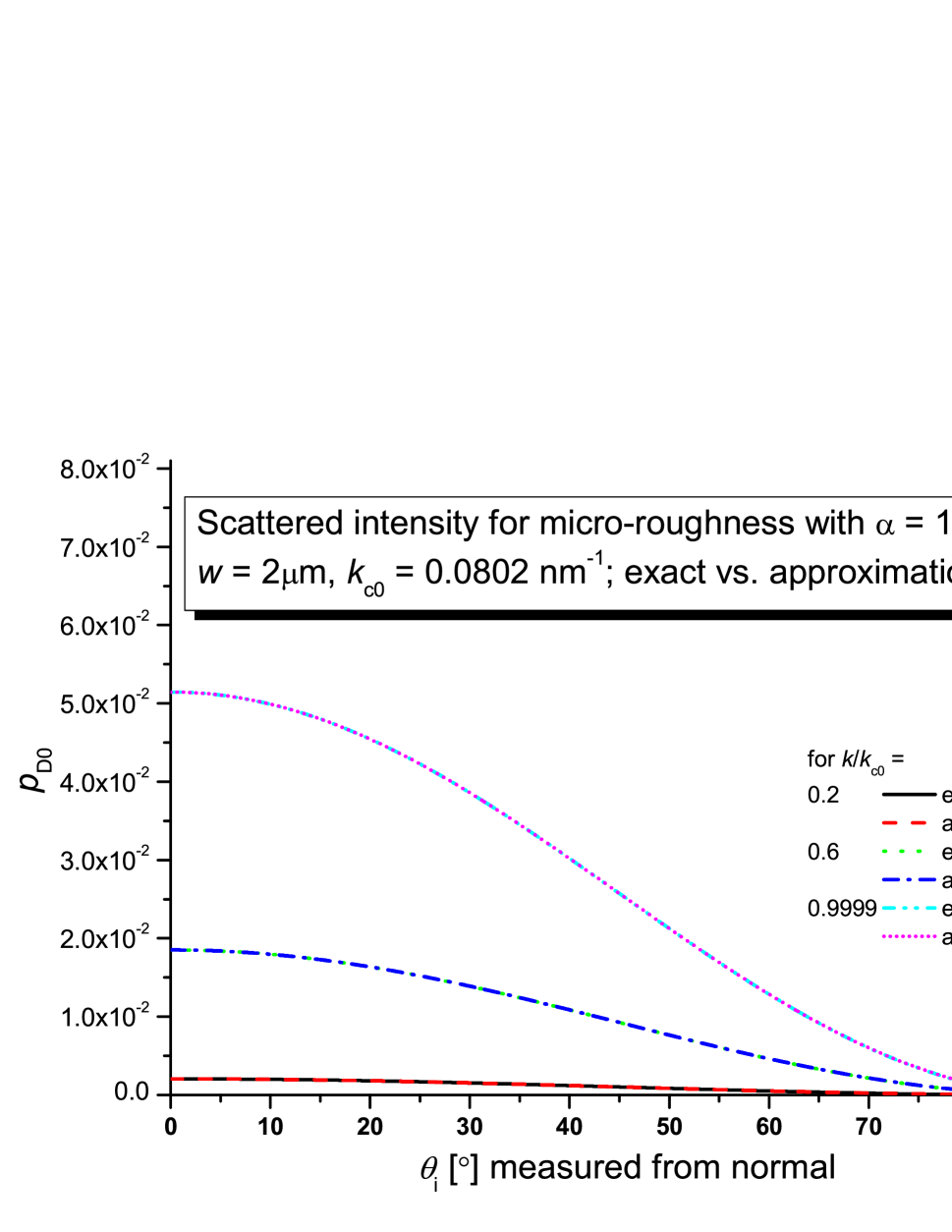
(1,1): The first order intensity scattered into unit solid angle at is given by the outgoing flux with density , normalized to the incident flux, with the result (for UCN)
(14) where
(15) is the Fourier transform of the height-height correlation function (1) and represents the roughness spectrum [4]. For , and for UCN (rather than cold neutrons in general) Eq. (14) agrees with Eq. (20) of [4]. Removing common constants, we write , where
(16a) (16b) From (14) we obtain the total diffusely scattered intensity, up to terms and :
(17) where
(18) is the total scattered intensity for , and is the flat-wall loss coefficient for angle . For the scattered intensity forms a halo around the specular beam with small width of order , as expected from ray optics.
- (d)
-
(0,2): Interference of specular reflection with second-order perturbation, arising from :
(19) For , this term is required to satisfy unitarity. Up to order , the total outgoing intensity (specular plus diffuse) equals the incoming intensity. In other words, the ’Debye-Waller’ attenuation factor DWF for the specular beam equals , as it should. Carrying out the integration for we find that the DWF is close to but not identical to the factor given in [5]. At this point it should also be mentioned (as is in [5]) that to arrive at the common Gaussian form for a DWF one has to make the drastic assumption that the wave inside the medium is given by the same function as the wave outside the medium, throughout the rough layer. This is not plausible for larger roughness, especially not for UCN, since only and its first derivative are continuous at the surface. Using (13) and (19) we obtain the Debye-Waller factor for an absorbing, rough wall: (up to terms and ).
- (e)
-
Combining the terms (0,0), (0,1), (1,1) and (0,2) we obtain the absorption coefficient for a rough wall:
= (incoming flux - outgoing flux)/(incoming flux) = 1 -(20) This agrees with the result derived in [7] using a somewhat different approach. Numerical results were not given in [7]. Higher-order perturbation would yield only terms with .
V Approximations and Numerical Results
Numerical evaluation of the double integrals over and in (17)-(20) is greatly facilitated if one of the integrations can be performed analytically. For the Gaussian model, the -integration leads to the Bessel function , but no analytical solution is known for the ‘-model’. Using the transformation , with , the -integration can be performed analytically for any roughness model since only depends on , not on . It is evident from Fig. 1 that for (with , the -integration runs from to . For , the limits are with . Expressing in terms of and as , the -integrations in (17)-(20) can be performed analytically in terms of elliptic integrals, as shown in Appendix D.
Before proceeding with numerical results, we point out the special case of fairly smooth surfaces with small mean-square slope and a UCN wavelength small on the scale of the lateral correlation length w, viz. . Smooth surfaces are expected to form when a special low-temperature oil ’LTF’ [10] is sputtered onto a cold surface, then thermally cycled by slow liquefaction and re-freezing, as in [3]. Under these circumstances, is very small for and the -integration can be extended to . In this case, model-independent results are obtained as follows: The analytical expressions for the -integrals are expanded for small as and we use the identities
| (21) |
| (22) |
| (23) |
which follow from the properties of Fourier transform (15) and relations (4) and (7) between and .
In this way asymptotic expressions are obtained for and :
| (24) |
and
| (25) |
where and . For perturbation theory to be valid, must be over the entire range of .
Taking only the first term in the curly bracket , Eq. (24) is consistent with the usual DWF with expansion , which is the standard Born approximation result of [5] (see also [12]). Note that for the loss of specular intensity, 1-DWF, equals [6], thus particle number is conserved. Figure 2 compares approximation (24) (first term only) with the exact numerical result for nm-1, and m ( nm). The critical value is for the LTF oil in its glass state at K used in [3]. The agreement is excellent, indicating that for these parameters the Born approximation for the DWF is adequate. The numerical values of for the Gaussian model are very similar to those of the -model used for Fig. 2.
On a general basis, for the approximations (24-25) are valid over a wide range of , but not near grazing incidence since in this range is . Therefore the -range for integration over the full -range from to (see Fig. 1) cannot be extended to .
From (25) we deduce a, perhaps, unexpected result: over a significant range of , namely where the curly bracket is positive (for : ), the loss coefficient for the rough surface, , is somewhat smaller than that for the flat wall, , with a relative difference of order . This contradicts a general statement in [7], p. 185, while a decrease was predicted for a certain model in [11]. The decrease found here for is independent of the model and is plausible for a geometric-optics picture, where geometric reflections for the local surface orientation are incoherently superposed: For near-normal incidence the mean angle for incidence on inclined patches of a rough surface is always larger than for the flat surface, for which it is zero for , and therefore the factor in is reduced, on average. No reduction of is seen for ’jagged’ roughness with of order 1.
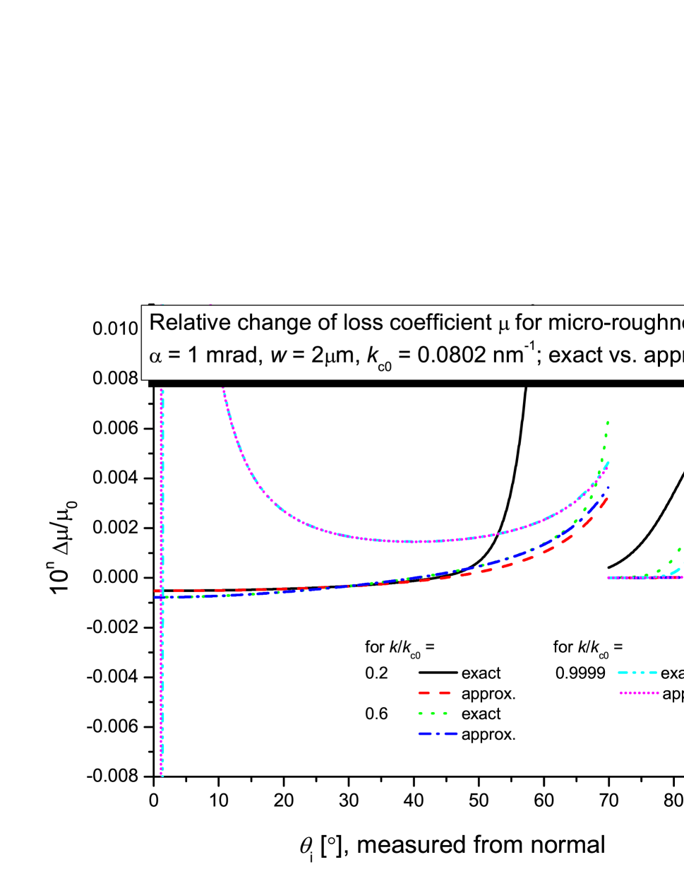
For the same values of , etc. as for Fig. 2, Fig. 3 shows a comparison of numerical results for with approximation (25) for the model. Again, the approximation clearly fails for grazing incidence (both (24) and (25) diverge as but is an excellent representation at steeper incidence. The Gauss and model give very similar results.
For UCN confined in a trap the angular distribution is, in most cases, assumed to be close to isotropic (although deviations are critical, see below). To obtain directional averages of and the region of grazing incidence that is not described by (24-25) has to be included, and it makes a significant contribution. The angular dependence of for the Gauss-model (not shown in Figs. 2 and 3) with the same parameters is close to that for the -model and the isotropic mean values
| (26) |
agree within 15 percent. Fig. 4 shows the -dependence of for both models. The reference average for the flat wall is given as [7-9]
| (27) |
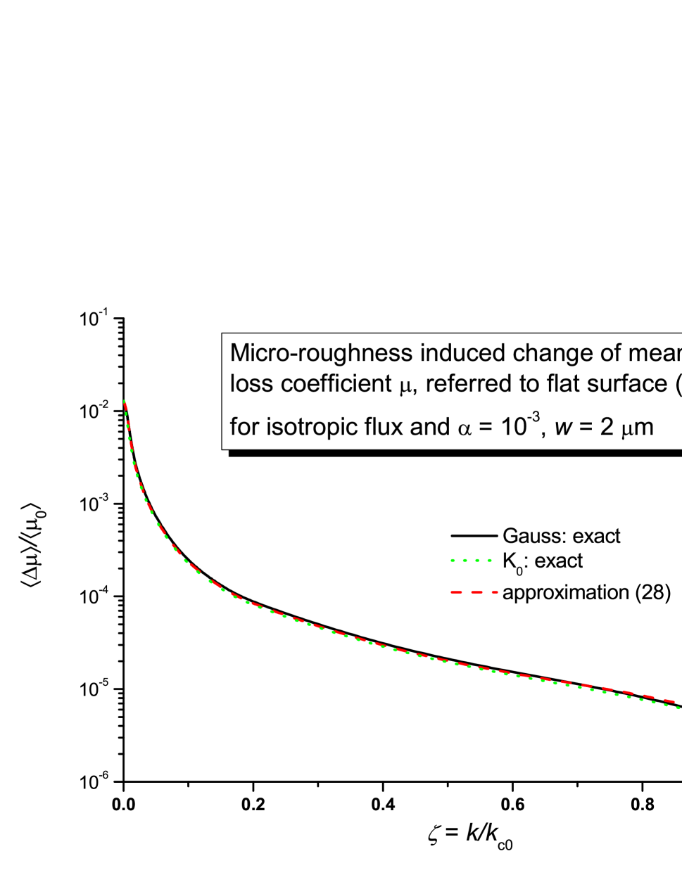
The main features of are a sharp peak of height at with half-width and a drop-off approximately . A reasonable fit, with maximum deviations of over a wide range of and of (small) and b and (large) w, both to the Gauss- and micro-roughness models, is
| (28) |
which is shown as the dashed curve in Fig. 4. The isotropic-flux average of diffuse fraction is
| (29) |
where we used the one-term approximation of (24).
In applications to actual UCN storage, approximations (28,29) can be used to determine further averages analytically. For a monochromatic UCN spectrum under gravity the averaging is over wall-interaction height h from the trap bottom to the ’roof’ or to the maximum height reachable for a given energy (, in units of maximum jump height). Further averaging over the spectrum (over ) is usually also required. For instance, the sharp peak of at implies a large loss rate for UCN in contact with the wall near their maximum jump height where . Taking into account that the flux [] incident on surface element dS vanishes as , a detailed analysis is required. It shows that the loss enhancement strongly depends on the trap geometry and UCN energy and is significant for very low energy UCN ’hopping’ in small jumps on an essentially flat horizontal surface, for instance the rim of a cylinder with horizontal axis, as in [3].
VI Detailed balance requirement and simplifications
A trapped UCN gas will acquire or maintain an equilibrium isotropic distribution only if its interaction with a rough wall (or magnetic field irregularities) satisfies the detailed balance requirement discussed in [7], p. 96. The flux undergoing scattering from solid angle to must equal the flux for the reverse process , in accordance with the fundamental principles of time-reversal invariance and micro-reversibility. Since the flux incident at (or ) is proportional to (respectively ) any diffuse scattering distribution ) must satisfy the symmetry requirement
| (30) |
where is a function symmetric in and and is the Lambert factor. The scattering distribution of Eq. (14) satisfies this requirement.
Various simplifications of the micro-roughness scattering distribution (14) (for ) have been used in [13-15]. The limit of maximal diffusivity is reached for a ”dense roughness” model where , hence . This leads to [14,15]
| (31) |
with and a diffuse fraction that depends on incident angle and UCN energy (). It has been pointed out in [15] that for at most of order 1, as required for perturbation theory to be valid [4], the limit , hence , is strictly justifiable only for very small diffuse fraction .
As a further simplification, averaging over incident energy may be performed but could be a coarse approximation for broad spectra, as for confined UCN. To arrive at the simplest form of (30), with , requires further averaging of in (31). Assuming isotropic distributions in and we obtain . Thus, (31) becomes
| (32) |
with and a total diffuse fraction . Like (31), Eq. (32) is justified only for small .
In the ”dense roughness” limit the loss coefficient of (20) can be averaged analytically [7] with the result , where is given in (27). However, except for very small the correction term would become large as , conflicting with the perturbation theory requirement.
It should also be noted that in averaging over we lose the proportionality of to which implies a small scattering probability for glancing incidence (). For UCN stored in traps with high geometrical symmetry this dependence can give rise to almost stationary orbits for UCN ”sliding” along a concave surface (see Sec. 8). For other geometries, only a few reflections, or where these details are not important, as in the computer code tests of [13], (32) is a useful, simple approximation satisfying detailed balance.
As an example of a roughness model that does not satisfy detailed balance we mention the scattering distribution (E6) derived in Appendix E for the macroscopic, ray optics limit. In this case, is symmetrical in and , lacking the extra factor . This violation of detailed balance can be tolerated if only a few reflections have to be considered, as in a neutron guide [4], but attempting to use this model for thousands of consecutive reflections in a Monte Carlo simulation, as required for long UCN storage (see below), results in the loss of isotropic equilibrium. We observed that UCN accumulated in grazing-angle orbits, depleting other regions of phase space.
VII Monte Carlo simulation techniques
In Monte Carlo simulations of UCN propagation and storage, as in [7,14,15], two complementary ways of implementing a given scattering probability distribution , e.g. Eq. (14), have been discussed and used.
One ([7], p. 98) is based on mapping the joint probability distribution onto the ranges 0 to 1 of uniformly distributed random numbers (r.n.) x, y, z, etc. For instance, for the ’dense roughness’ limit of Eq. (14) used in [14] in the form , we can determine and from x, y, setting and . In general, the mapping procedure involves indefinite integrals of and becomes very tedious if numerical integrations are required as for (14). In the simple case the indefinite integral is , hence the prescription . Rendering this method efficient requires 3D tabulation where the tables need only be interpolated at each UCN reflection during a simulation run. As a further simplification, once has been determined, is found faster from the conditional probability of , given : , where is the integral probability for . For the Gaussian model the numerical work involves only the incomplete Bessel function, which is readily available in computer code.
For our simulation (below) we chose the second, often faster method used in [15], to determine and in a way consistent with the probability distribution. First read from a table the total diffuse-scattering probability for given incidence parameters k and . A r.n. then determines whether the reflection is specular (if ) or diffuse (). If diffuse, a trial set is obtained as and . Next, find the probability for the trial set and compare it to a fourth r.n., z. The angles are accepted if , where is the maximum of for incidence at k and . If , the process is repeated with new r.n.’s x,y,z. This scheme can be greatly abbreviated if . In this case rolling three dice only once is sufficient. x and y determine and , as before. If , the reflection is specular, otherwise diffuse at angles . It can be verified that this faster scheme also respects the probability distributions correctly (as long as ).
In all these schemes, wall losses and beta-decay are irrelevant for the choice of reflection angles. However, we keep track of the accumulation of net loss at each reflection and use the overall loss factor as a weighting factor for UCN that have survived losses and can be counted in a detector. The loss factor contained the second-order correction of Eq. (20) and was implemented in tabulated form.
VIII Monte Carlo simulation for neutron lifetime experiment [3]
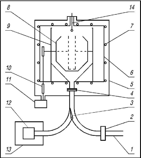
The neutron lifetime experiment [3] reports a value s which is 7.2 s (or , or standard deviations) away from the current particle data world average s [2]. The quoted precision is better than for any previous single lifetime measurement. Since data interpretation for this experiment relied heavily on computer simulations we have performed independent simulations using the roughness model outlined above. In this system [16,3], shown in Fig. 5, a cylindrical or a ’quasi-spherical’ vessel with an opening rotates about a horizontal axis during the various steps of a cycle: Filling with UCN with the hole pointing straight down; rotation to a ’monitoring position’ for spectral cleaning; storage for a ’short’ time (300 s) or a ’long time’ (2000 s) with the hole in the upright position; then emptying in 5 steps at intermediary angles. This scheme provides for a spectral analysis, with a batch of higher-energy UCN counted first and the slowest UCN pouring out at the last stage while the opening moves to the vertical down position. The detailed measuring scheme [3] is complex, involving not only energy dependent data for the 5 energy bins but also traps with different mean free path for the UCN. This combination allows, both ’energy extrapolation’ and ’size extrapolation’ to the neutron lifetime.
Data analysis is also complex, relying heavily on computer simulation to determine the parameter against which measured inverse storage lifetimes are plotted for the extrapolation. The average , with wall collision frequency f, is the wall loss rate (mean loss per second).
For a narrow cylindrical trap the authors of [3] compared simulations with the measured time spectra for the first counting interval following short storage (300s) (see Fig. 14, lower part, of [3]). They concluded that a certain minimum roughness (diffuse fraction ) of the trap wall was required to obtain agreement. This is a crucial step with respect to the neutron lifetime, and therefore we have performed independent simulations of short and long storage cycles for a narrow cylindrical vessel with radius 38cm, width 14cm, and aperture for the opening, to investigate this issue using the near-mirror reflection model with long-range roughness () described above.
In our simulation UCN are generated at the beginning of the monitoring phase (at trap angle ) over a horizontal area inside the trap volume and near its bottom. The distribution is isotropic with polar angle , referred to the up and down directions, derived from a r.n. x as . The energy distribution is the same as used in [3], namely the Maxwell distribution modified by a heuristic attenuation factor with m (not specified in [3]). We used a maximum (minimum) energy of 0.95 m (0.05 m).
The time sequence of monitoring, storage and emptying in five steps was the same as described in [3]. The wall reflections were assumed elastic except for the (very small) Doppler shift for wall reflections during times when the trap rotates at s (respectively s on the way from to for a rotation time of 2.3s [3]) and the reflection is diffuse. For perfectly cylindrical geometry the overall shift is very small. Reflection points were calculated analytically from the previous reflection position, energy and take-off angle, assuming perfectly cylindrical geometry. At each reflection, the wall loss was incremented according to the loss coefficient for this reflection. A run was terminated at the time when the UCN passed through the opening without immediately falling back into the trap. For the purpose of this work the exit channel could be neglected and those UCN that had escaped loss, as determined by the integrated loss including beta-decay, were counted into time bins of 10s or 1s resolution. For consistency with [3] we used the quoted values and s in the simulation. The bins were combined to the five counting intervals, and short runs with storage time 300 s were compared to long runs (2000 s) as in the actual experiment to obtain the storage lifetime as a function of mean values that were also calculated for each counting interval.
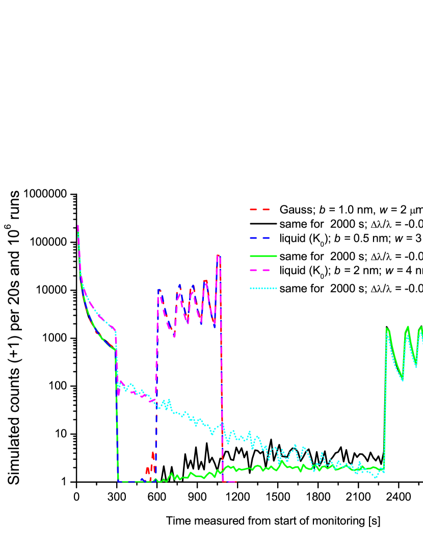
Figure 6 shows simulated count rates, in 20 s bins, versus cycle time t, starting from ’monitoring’ for 300 s where the trap is at position tilted away from vertical. The data are normalized to runs (one run for each UCN started at t = 0). Data are shown for both short and long storage and for both the Gauss and models, for a fairly smooth surface with similar parameters, as shown in the inset. They correspond to for the Gauss-model, and for . An example of steeper roughness with (for nm and nm) is shown for comparison.
We will focus on two features of Fig. 6, and their implications: first the time spectra for the first counting interval following short storage; then the count-rates during long storage.
First counting peak
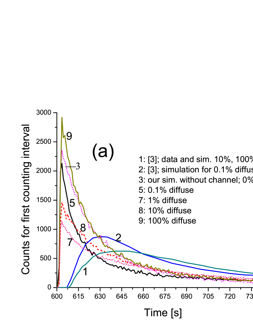
To allow a comparison with the time spectra for the first peak measured in [3], we show in Fig. 7, at a higher resolution of 1 to 2s, an expanded view of the interval from 600 to 750s (on the time scale of Fig. 14 of [3] this corresponds to the interval 740 to 890s). The data of [3] are included in Fig. 7 as curves 1 and 2. Prior to discussion we point out differences between the two simulation approaches.
|
|
The authors of Ref. [3] used a roughness model characterized by a single number, the diffuse fraction for the trap walls, but did not state which roughness model was used. The simulation included the exit channel (designated secondary volume and UCN guide in [3]) but the authors did not describe the geometrical model used for this complex structure. It included (see Fig. 5) the trap exterior and interior (which some UCN temporarily re-enter on their way to the detector), the wide conical channel section, the valve selector with its gaps, the curved guide and the detector with its window that accumulated an oil film as a result of repeated surface coating using the evaporator 14 shown in Fig. 5. The surface properties, including roughness, of the oil-coated channel walls with their temperature gradient, varying from the trap temperature to near-room temperature for the detector, are not discussed.
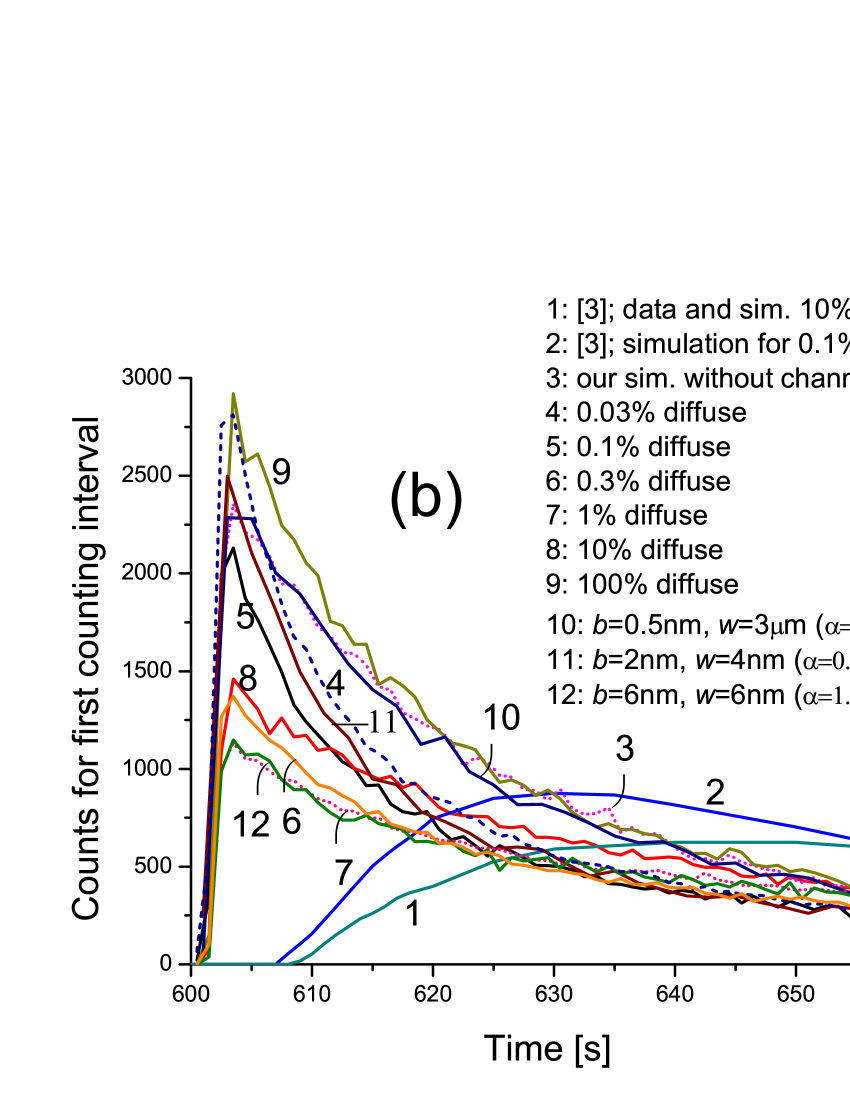
Our simulation did not include the exit channel. We used the roughness models and parameters listed for curves 3-12 of Fig. 7. In Fig. 7b the initial part is expanded for clarity. For these counting spectra following short storage the details of wall loss are insignificant and the results using (20) are indistinguishable from those for the elementary, flat-wall expression that was used in [3]. (During the long holding period of 2000s the details of loss coefficient may become important, depending on the roughness parameters.)
Curve 1 represents the measured data (Fig. 14 of [3]), using a scale approximately adjusted to counts per 2s for initial UCN. Curve 1 practically coincides with the Ref. [3] simulations for 10% and 100% diffusivity. Curve 2 is the simulation, in [3], for 0.1% diffusivity. Curve 3 is our simulation (for the trap only) for an ideally smooth surface. For curves 4-9 we used the simplest scattering distribution consistent with detailed balance, Eq. (32), with diffuse fractions 0.03, 0.1, 0.3, 1, 10 and 100%. For consistency with [3], we included large values of , disregarding the restriction outlined following Eq. (31). Curves 10-12 are based on the micro-roughness result (14) (for ) and the -model. The parameters for curves 10-12 represent increasingly steeper roughness (, 0.71, and 1.4) and increasing (0.16, 0.55, and 11.3%, where the last value is at the limit of perturbation theory validity).
Fig. 7 shows the large spectral distortion and time delay due to the exit channel. The peak widths at half maximum for curves 1 and 2 are 3 to 6 times larger than for the simulations excluding the exit channel. Thus the channel response function to the relatively short pulse of UCN pouring out of the trap essentially determined the measured time spectra.
For consistency with [3] we focus first on the simulations based on (32). The minimum half-width =10s is observed for =0.1%. Both for 1% and (including zero), the curves are 2 times wider, while the curves for 0.03% and 0.3% are intermediary. The difference between 0.1% and 1% diffusivity makes plausible the (much smaller) difference of broadened peaks between the Ref. [3] simulations (including the channel) for =0.1% (curve 2) and 10 or 100% (curve 1). Comparing to the measurement the authors rejected the possibility of diffusivity for the trap. However, curve 3, for =0, has about the same larger width, namely =23s, as for 1% (curves 7-9).
The same type of broad line is seen for curve 10 that is based on Eq. (18) for small . The intermediate (steep) roughness model used for curve 11 (12) results in intermediary (broad-type) linewidths.
The difficulty of distinguishing between roughness models for the trap on the basis of measured curves broadened 3 to 6 times by the response, or resolution, function is exacerbated by two aspects: First, by the uncertainty introduced by any simplification of the complex channel geometry, as needed to make the simulations feasible. Secondly, in this experiment (and perhaps any UCN experiment conducted so far) neither the primary source intensity and spectrum nor the transmission characteristics of connecting guide tubes, shutters and other components, here including the channel that is passed by the UCN also during trap loading, is known well in absolute terms. Thus, the area under the counting peak can practically not be used as a criterion for adoption or rejection of a roughness model for the trap. In the present case, the observed variation of peak area in Fig. 7 is a reflection of spectral mixing between the five spectral intervals, as discussed below.
We conclude from this peak analysis that a ”soft-roughness” model with , as is expected for the temperature-cycled [3] oil-glass coating used, can, probably, not be excluded. This has the consequences outlined below.
’Spill-over’ during long storage
Returning to Fig. 6, we draw special attention to the finite count rate that appears during the storage intervals, t = 300 to 600 s for short storage and t = 300 to 2300 s for long storage. At the end of monitoring at trap angle most UCN with energies exceeding the height barrier ( cm above trap bottom) have spilled out. However, some higher energy UCN move, preferentially, along the cylinder axis and little in other directions. In this highly symmetric trap geometry they have survived in nearly stationary orbits since, for , the reflections are nearly mirror-like with small reorientations of order if the reflection is diffuse. Thus the random walk toward isotropy is very slow. As the trap rotates to angle at s the barrier rises by 14 cm to 70.5 cm from the bottom, and the count-rate in Fig. 6 drops to zero. However, since UCN with energies exceeding this new barrier still remain, the same slow relaxation toward isotropy gradually results in steeper orbits. At s some UCN have reached the new barrier and we see a fairly constant ’background’ count rate throughout the remainder of the long storage interval up to s. The range of parameters , b and w showing this general tendency is fairly broad, and there is no qualitative difference between Gauss and models. We will show that this ’background’ could be overlooked in actual measurements. The same slow diffusion in phase space is also expected to mix the spectral regions for the five counting intervals, and the net result of slow relaxation could give rise to a significant systematic error.
For comparison with experiment [3] we note that the counts in Fig. 6, for runs, correspond to double cycles (one cycle each for short and long storage). The instrument background of 0.02 s-1 (Fig. 10 of [3]) is equivalent to 5 counts/20 s in the region 600 s 2300 s of extra holding time for long storage in Fig. 6. This interval has no counts without the relaxation process since the instrument background was not included in our simulations. Thus, the UCN ’spilling over the threshold’ during this time ( 0.8/20 s, or 67 in total for the model) are missing from the UCN count, , following long storage, but are not missing from the short-storage counts . In the actual experiment the relative change of measured ’background’ (0.8/5 ) is below the significant background variations shown in Fig. 10 of [3] and would hardly be noticed. However, calculating from an inverse storage lifetime, , with = 2300 s -600 s = 1700 s, disregards the ’spill-over’ and would result in a significant uncertainty of , as shown in the following estimation.
We assume that the spill-over rate originates exclusively from the highest-energy interval (of the 5 intervals) and that entry into (exit from) spectral interval by angular diffusion from (into) , or any other interval, is negligible. Thus the number of UCN in decreases during long storage as
| (33) |
In [3] is close to the lifetime , so we can approximate by in the last term of (33). Integrating (33) from to and equating with the counts for interval , , and with we obtain
| (34) |
The first term on the right is the -value disregarding spill-over. The second term is the correction with
| (35) |
where the sum is over the count rates from to , with a weight factor . Finally, the correction becomes
| (36) |
This value is given in the inset of Fig. 6 and amounts to significant corrections to the inverse storage lifetime for interval . If inter-interval diffusion is included the values for other spectral intervals, and presumably the energy extrapolation as well, are affected to a significant extent. On the other hand, the measuring scheme of [3] is more complex, involving also the larger traps including a ’quasi-spherical’ vessel, which in the simulations was replaced by a cylinder in a way not discussed in [3]. We will point out below that our simulation for a fairly smooth surface of a narrow cylindrical trap leads to questions also regarding the x-values of the extrapolation, namely the mean values for the spectral intervals 1-5.
For the example with steeper roughness in Fig. 6, relaxation is faster and the large ’back-ground’ in the region 300 s t 600 s might be visible in the experimental data, in spite of blurring by the exit channel.
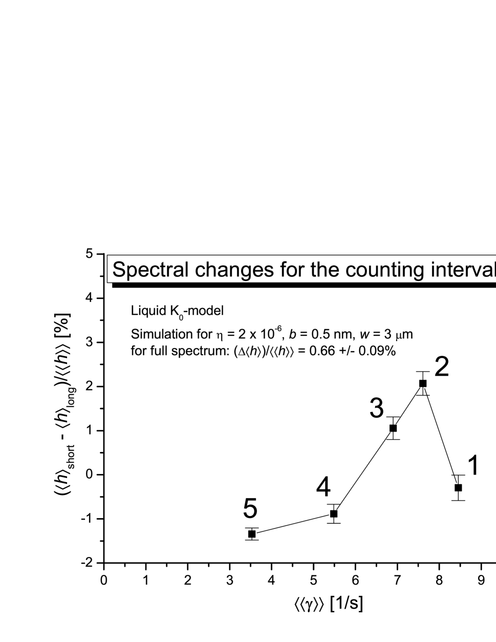
Mean -values
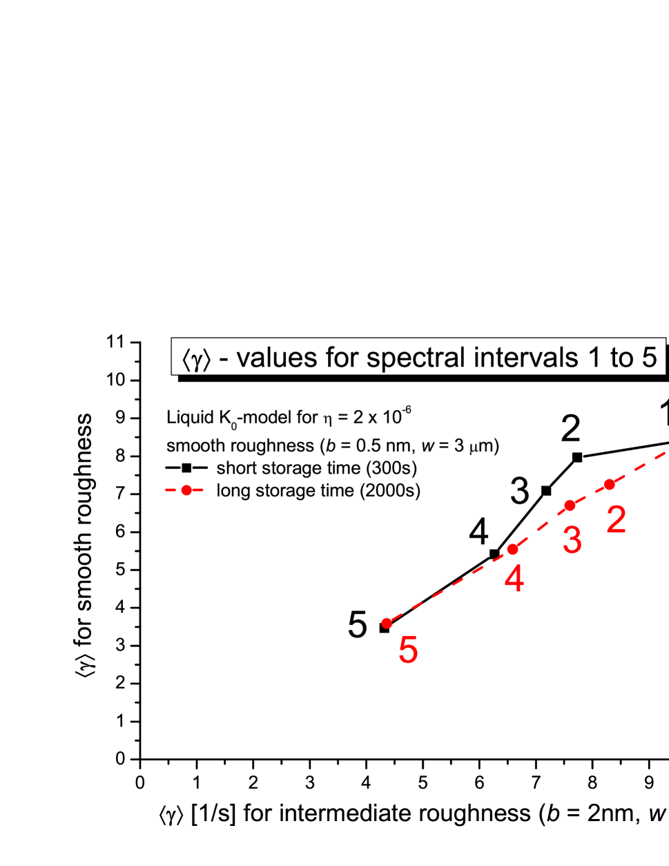
For the narrow cylindrical vessel, Fig. 8 combines values for the five spectral intervals: on the x-axis for an ’intermediate’ roughness with nm and nm, and on the y-axis for a ’smooth’ roughness with nm and m. The data for short and long storage are plotted separately and the differences are seen to be substantial. They are not explained by the small spectral cooling during storage due to larger wall losses for higher UCN energies. Spectral mixing and spill-over are more important. The large differences are also seen in the mean collision frequencies (not shown) for the five intervals.
Mean spectral energies
Spectral mixing is also seen in the ’erratic behavior’ of mean spectral energies (height and difference, , between short and long storage). In Fig. 9, is plotted versus (averaged over long- and short storage) for the ’smooth’ roughness parameters. A spectral change between short and long storage implies a change of detection efficiency that is not discussed in [3]. While the difference in mean UCN velocity is reduced by the energy boost through the fall height of m between storage vessel and detector, the transparency of the oil coated detector window for an isotropic UCN beam is a steep function of velocity in the region of interest, with roughly a change of 4% for 1% of UCN energy change. As a result the UCN spend more time in the entrance/exit channel and have a greater chance of being lost, for instance through gaps.
IX Conclusions
Using models of microscopic roughness characterized by height-height correlation functions of the Gauss and ’’ type (for solid vs. liquid surfaces) we have carried perturbation calculations to second order, recovering a previous result [7] for roughness-induced wall loss for UCN that has, apparently, found no attention so far. It may be surprising that under certain conditions roughness reduces the wall loss probability. Furthermore, the second-order approach provides absorption corrections to the diffuse scattering distribution as well as the leading terms of a ’Debye-Waller factor for roughness’ that is consistent with previous derivations but does not require the additional assumption of a height probability distribution function made, e.g., in [1] and [5]. It is shown that for a fairly smooth wall with small mean-square slope the results are model independent and are determined only by the mean values, mainly for height () and slope ().
As the central application of roughness scattering we describe independent simulations relating to neutron lifetime experiment [3] which reported a significant deviation from the world average and very high precision. The possibility of a fairly smooth surface for the temperature cycled oil used as the wall coating in this experiment, in connection with the possibility of nearly stationary orbits in any highly symmetric trap geometry, raises questions about the reliability of the extrapolation method used to extract the lifetime value from the storage data.
Acknowledgements.
We acknowledge very useful discussions with B. G. Yerozolimsky, G. Müller, R. Golub, E. Korobkina, A. V. Strelkov and V. K. Ignatovich. We thank N. Achiwa for measuring the temperature dependence of the scattering potential for the LTF oil.Appendix A Correlation functions
Application of the Laplace operator twice in Eq. (7) yields for the Gauss model:
| (37) |
with mean square curvature
Using properties of the modified Bessel functions (with ) we obtain for the model.
| (38) |
with
| (39) |
and
| (40) |
The expressions for the mean squared curvature hold for the choice , for which the two models have identical mean-square slope . This value of is the solution of .
Appendix B Green’s function for a flat surface
Eq. (10) describes the wave, with wave number k, generated at point by a point source at near the surface of a semi-infinite slab of material with scattering potential . The solution may be represented by a Fourier expansion in terms of in-plane waves as [17]
| (41) |
The one-dimensional Green’s function for satisfies the equation
| (42) |
where the wave number component perpendicular to the wall is , and in vacuum and inside the medium. For UCN with , is imaginary apart from a very small real part due to the loss contribution in . The solution of (B2) for outgoing plane waves can be written, for , :
| (43) | |||||
and for , :
| (44) | |||||
with .
(B3) and (B4) were derived assuming . The two-term approximations in (B3) and (B4) are valid for ’micro-roughness’, where , and they hold for positive or negative values of within the rough layer. This is a direct consequence of the continuity of and at the interface. We note that the first two expansion terms are sufficient for a full description of UCN interaction with a rough wall up to terms quadratic in the roughness amplitude b.
The same kind of approximation can be made for the plane-surface wave in the integral of Eq. (9). Thus, using (B3) the -integral in (9) from up to the roughness amplitude across the rough layer is proportional to where .
The full Fourier expansion (B1) is needed in (9) in second-order perturbation where the first-order perturbation obtained for in (9) is subsequently inserted in the integral with replaced by to obtain .
For flux calculations, we need the far field expressions for for . Using the two-term approximation for its z’-dependence (the last bracket in (B3)), Eq. (15) of ref. [4] reads
| (45) |
Appendix C perturbation calculation up to second order
Derivation of the results listed in section 4 is lengthy and we will only summarize a few crucial steps, using the same symbols as in the text.
- (a)
-
Integrations over :
By definition of :(46) By definition (1):
(47) By definition (15):
(48) - (b)
-
UCN flux:
Incoming flux for velocity (with m = neutron mass):
(49) Outgoing flux into solid angle :
(50) For the specular beam at angle
we can use the plane wave expansion in spherical harmonics [18] for large distance r:
(51) This allows simple integration of the interference integrals.
- (c)
-
Loss terms:
On each step the terms containing the loss coefficient are developed to first order in . For instance, for not too close to :(52) with and
Appendix D Integrations in q-space
Using the transformation and the relationship
the integrations over in (17)-(20) can be performed analytically. The integrations run from 0 to where
| (53) |
Since the -integrals needed in (18) to (20) do not appear to be readily available from tables or websites we list two results
| (54) |
and
| (55) |
where [19]
| (56) |
is the incomplete elliptic integral of the first kind,
| (57) |
is the incomplete integral of the second kind, and
and
are the corresponding complete
elliptic integrals of the first and second
kind, respectively. The arguments in (D2) and (D3) are
; ;
; ; ;
;
Compared to numerical double integration, the use of these readily available functions in one of the integrals as well as tabulation of the numerical results for use in simulations is of enormous benefit.
Appendix E Macroscopic limit
In the geometrical optics model, reflection is considered as an incoherent superposition of rays reflected at each speck of a fairly smooth surface () as if it were a plane inclined at the local slope. The analysis is based on a slope distribution function that has to be postulated independently of the correlation function . For instance, does not have to be Gaussian if has been chosen Gaussian. If the simplest Gaussian is chosen, as in [4], it is of form
| (58) |
which is normalized and has the correct second moment The ambiguity is more obvious for the model. Requiring that should be a monotonic, bounded function, exhibit an asymptotic K-Bessel function behavior and, for convenience, be amenable to analytic analysis we can choose
| (59) |
where . For any , values of and can be determined analytically [20] such as to satisfy the normalization and second moment criteria. For : and where is the solution to . For small values of , the K model, as compared with the Gauss model, describes a surface with higher probability of large slope () at the expense of areas with a very small slope.
In the macroscopic-roughness model the probability of scattering (local reflection) from to , i.e. from angles to , at suitably oriented surface elements is :
| (60) |
The mapping involves the local polar angle of incidence, , where
| (61) |
with . We obtain
| (62) |
Inserting (E5) and (E1) into (E3) gives the scattering distribution. For the Gaussian model,
| (63) |
where the in-plane momentum transfer q is given in (11).
Eq. (E6) is consistent with the limiting case analyzed in ref. [4] (Eq. (26) of [4]) and it closely resembles the micro-roughness result (14) for (for ). It exhibits a similar width of scattering distribution around the regular reflection angle but no exactly specular intensity. Local angle dependent loss could be incorporated in the form as for a plane surface, but the result is not identical to the micro-roughness result in the limit .
Expression (E6) and similar expressions for non-Gaussian models are symmetric in and , thus do not satisfy the detailed balance requirement discussed in Section 6, and indeed give rise to loss of isotropy in computer simulations. Moreover, (E6) is catastrophically inadequate for glancing-angle incidence () due to shadowing and multiple reflection within a rough surface as discussed in Section 6. Although this angular range is small, it makes a large contribution to the mean value for isotropic incident UCN flux and cannot be neglected.
References
- (1) P. Croce, L. Névot, B. Pardo, C.R. Acad. Sci. Paris 274, 803 and 855 (1972).
- (2) C. Amsler et al., (Particle Data Group), The Review of Particle Physics, Phys. Lett. B667 (2008).
- (3) A. Serebrov et al., Phys. Lett. B 605, 72 (2005); and extended version of PNPI preprint 2564 (2004) [our references relate to the latter version]; also in A.P. Serebrov et al., Phys. Rev. C 78, 035505 (2008) .
- (4) A. Steyerl Z. Physik 254, 169 (1972).
- (5) S. K. Sinha, E. B. Sirota, S. Garoff and H. B. Stanley, Phys. Rev. B 38, 2297 (1988).
- (6) A. Steyerl, S. S. Malik and L. R. Iyengar, Physica B 173, 47 (1991).
- (7) V. K. Ignatovich, The Physics of Ultracold neutrons, Clarendon, 1990, esp. Appendix 6.10, and personal communication.
- (8) A. Steyerl, Very low energy neutrons, in Neutron Physics, Springer Tracts in Modern Physics, 80, 57-127 (1977).
- (9) R. Golub, D. Richardson, S. K. Lamoreaux, Ultra-Cold neutrons, Hilger (1991).
- (10) A. Steyerl, B. G. Yerozolimsky et al., Eur, Phys. J. B 28, 299 (2002).
- (11) A. V. Stepanov, Teor. Mat. Fiz. 22, 425 (1975).
- (12) Using a Distorted Wave Born Approximation, the expression was obtained in [1] and [5], where the primed quantities refer to the quantities inside the refractive medium. This modification is clearly inapplicable within the total reflection range, where is imaginary (approaching zero at the edge).
- (13) F. Achison et al., Nucl. Instr. Meth Phys. Res. A 552, 513 (2005);
- (14) I. Berceanu and V. K. Ignatovich, Vacuum 23, 441 (1973).
- (15) M. Brown, R. Golub and J. M. Pendlebury, Vacuum 25, 61 (1975).
- (16) P. Geltenbort et al., http://surface.phys.uri.edu/Publications-Steyerl/list/n-lifetime.2003.pdf
- (17) P. M. Morse and H. Feshbach, Methods of theoretical physics, McGraw Hill, 1953, ch.7.
- (18) A. Messiah Quantum Mechanics, Vol. 1, Wiley 1961, Appendix B. 10.
- (19) M. Abramowitz and I. A. Stegun, Handbook of mathematical functions, Dover, 1970.
- (20) I. S. Gradshteyn amd I. M. Ryzhik, Table of integrals, series, and products, Academic (1980), Eq. 6.596.7.