Instantons revisited: dynamical tunnelling and resonant tunnelling

Abstract

Starting from trace formulae for the tunnelling splittings (or decay rates) analytically continued in the complex time domain, we obtain explicit semiclassical expansions in terms of complex trajectories that are selected with appropriate complex-time paths. We show how this instanton-like approach, which takes advantage of an incomplete Wick rotation, accurately reproduces tunnelling effects not only in the usual double-well potential but also in situations where a pure Wick rotation is insufficient, for instance dynamical tunnelling or resonant tunnelling. Even though only one-dimensional autonomous Hamiltonian systems are quantitatively studied, we discuss the relevance of our method for multidimensional and/or chaotic tunnelling.

I Introduction: events occur in complex time

Instantons generally refer to solutions of classical equations in the Euclidean space-time, i.e. once a Wick rotation $t\mapsto-{\mathrm{i}}t$ has been performed on time $t$ in the Minkowskian space-time. Since the mid-seventies, they have been extensively used in gauge field theories to describe tunnelling between degenerate vacua Shifman94a . In introductory texts (Coleman85a, ; ZinnJustin02a, , for instance), they are first presented within the framework of quantum mechanics: when the classical Hamiltonian of a system with one degree of freedom has the usual form

$$H(p,q)=\frac{1}{2}\,p^{2}+V(q)$$ (1)

($p$ and $q$ denote the canonically conjugate variables), the Wick rotation induces an inversion of the potential and, then, some classical real solutions driven by the transformed Hamiltonian $p^{2}/2-V(q)$ can be exploited to quantitatively describe a tunnelling transition. As far as we know, in this context, only the simplest situations have been considered, namely the tunnelling decay from an isolated minimum of $V$ to a continuum and the tunnelling oscillations between $N$ degenerated minima of $V$ that are related by an $N$-fold symmetry. In those cases, what can be captured is tunnelling at the lowest energy only. However, not to speak of the highly non-trivial cases of tunnelling in non-autonomous and/or non-separable multidimensional systems, there are many situations that cannot be straightforwardly treated with a simple inversion of the 1d, time-independent, potential.

First, tunnelling — i.e. any quantum phenomenon that cannot be described by real classical solutions of the original (non Wick-rotated) Hamilton’s equations — may manifest itself through a transition that is not necessarily a classically forbidden jump in position Davis/Heller81b . For instance, the reflection above an energy barrier, as a forbidden jump in momentum, is indeed a tunnelling process Maitra/Heller96a ; Maitra/Heller97b . In the following, we will consider the case of a simple pendulum whose dynamics is governed by the potential $V(q)=\gamma\cos q$; for energies larger than the strength $\gamma>0$ of the potential, one can observe a quantum transition between states rotating in opposite direction while two distinct rotational classical solutions, obtained one from each other by the reflection symmetry, are always disconnected in real phase-space.

A second example is provided by a typical situation of resonant tunnelling: when, for instance, $V$ has a third, deeper, well which lies in between two symmetric wells (see Fig. 6a), the oscillation frequency between the latter can be affected by several orders of magnitude, when two eigenenergies get nearly degenerate with a third one, corresponding to a state localised in the central well. Then, we lose the customary exponential weakness of tunnelling and it is worth stressing, coming back for a second to quantum field theory, that having a nearly full tunnelling transmission through a double barrier may have drastic consequences in some cosmological models. In this example, one can immediately see (Fig. 6b) that $-V$ also has an energy barrier and working with a complete Wick rotation only remains insufficient in that case.

In order to describe the tunnelling transmission at an energy $E$ below the top of an energy barrier, which may be crucial in some chemical reactions, the pioneer works by Freed Freed72a , George and Miller George/Miller72a ; Miller74a , have shown that the computation of a Green’s function $\tilde{G}(q_{f},q_{i};E)$ (or a scattering matrix element) requires taking into consideration classical trajectories with a complex time. These complex times come out when looking for the saddle-point main contributions to the Fourier transform of the time propagator,

$$\tilde{G}(q_{f},q_{i};E)=\frac{1}{\sqrt{2\pi\hbar}}\int_{0}^{\infty}G(q_{f},q_{i};t)\,\mathrm{e}^{{\mathrm{i}}Et/\hbar}\;\mathrm{d}t\;,$$ (2)

which is, up to now, the common step shared by all the approaches involving complex time (Weiss/Haeffner83a, ; Carlitz/Nicole85a, ; Ilgenfritz/Perlt92a, ; Maitra/Heller97a, ; Creagh/Whelan99a, , for instance). Though well-suited for the study of scattering, indirect computations are required to extract from the poles of the energy Green’s function (2) some spectral signatures of tunnelling in bounded systems. Generically, these signatures appear as small splittings between two quasi-degenerate energy levels and can be seen as a narrow avoided crossing of the two levels when a classical parameter is varied Ozorio84a ; Farrelly/Uzer86a ; Heller95a ; Tomsovic98b . In the present article, we propose a unified treatment that provides a direct computation of these splittings (formulae 9 or 10); as shown in section II, it takes full advantage of the possibility of working not necessarily with purely imaginary time, but with a general parametrisation of complex time as first suggested in Mclaughlin72a . The semiclassical approach naturally follows (sec. III) and some general asymptotic expansions can be written (equations (101) and (40)) and simplified (equation (73)); they constitute the main results of this paper. To understand where these formulae come from and how they work, we will start with the paradigmatic case of the double-well potential (sec. IV) and the simple pendulum (sec.V); we defer some general and technical justifications in the appendices. Then we will treat the resonant case in detail in sec. VI, where an appropriate incomplete Wick rotation $t\mapsto\mathrm{e}^{-{\mathrm{i}}\theta}t$ provides the key to showing how interference effects à la Fabry-Pérot between several complex trajectories reproduce the non-exponential behaviour of resonant tunnelling, already at work in open systems with a double barrier Bohm51a ; Zohta90a . After having shown how to adapt our method to the computations of escape rates from a stable island in phase-space (sec. VII), we will conclude with more long–term considerations by explaining how our approach provides a natural and new starting point for studying tunnelling in multidimensional systems.

II Tunnelling splittings

A particularly simple signature of tunnelling can be identified when the Hamiltonian has a two fold symmetry and, therefore, we will consider quantum systems whose time-independent Hamiltonian $\hat{H}=H(\hat{p},\hat{q})$ commute with an operator $\hat{\mathsf{S}}$ such that $\hat{\mathsf{S}}^{2}=1$ (the $\ \hat{}\$ allows to distinguish the quantum operators from the classical phase-space functions or maps). In most cases, $\hat{\mathsf{S}}$ stands for the parity operator:

$$H(-p,-q)=H(p,q)\;.$$ (3)

The spectrum of $\hat{H}$ can be classified according to $\hat{\mathsf{S}}$ and, for simplicity, we will always consider a bounded system whose discrete energy spectrum and the associated orthonormal eigenbasis are defined by

$$\hat{H}\mathinner{|{\phi_{n}^{\pm}}\rangle}=E_{n}^{\pm}\mathinner{|{\phi_{n}^{\pm}}\rangle}\;;\quad\hat{\mathsf{S}}\mathinner{|{\phi_{n}^{\pm}}\rangle}=\pm\mathinner{|{\phi_{n}^{\pm}}\rangle}$$ (4)

where $n$ is a natural integer. When the Planck constant $\hbar$ is small compared to the typical classical actions, standard semi-classical analysis Takahashi/Saito85a ; Heller89a ; TorresVega/Frederick90a shows that one can associate some classical regions in phase-space to each eigenstate $\mathinner{|{\phi_{n}^{\pm}}\rangle}$. This can be done by constructing a phase-space representation of $\mathinner{|{\phi_{n}^{\pm}}\rangle}$, typically the Wigner or the Husimi representation, and look where the corresponding phase-space function $\phi_{n}^{\pm}(p,q)$ is mainly localised (all the more sharply than $\hbar$ is small). For a Hamiltonian of the form (1) where $V$ has local minima, some of the eigenstates remain localised in the neighbourhood of the stable equilibrium points. For instance, for a double-well potential whose shape is shown in Fig. 1a), the symmetric state $\mathinner{|{\phi_{n}^{+}}\rangle}$ and the antisymmetric state $\mathinner{|{\phi_{n}^{-}}\rangle}$ at energies below the local maximum of the barrier have their Husimi representation localised around both stable equilibrium points $(p,q)=(0,\pm a)$, more precisely along the lines $H(p,q)=E$ (1d tori) at energy $E\simeq E^{+}_{n}\simeq E^{-}_{n}$. Because of the non-exact degeneracy of $E_{n}^{+}$ and $E_{n}^{-}$, any linear combination of $\mathinner{|{\phi_{n}^{+}}\rangle}$ and $\mathinner{|{\phi_{n}^{-}}\rangle}$ constructed in order to be localised in one well only will not be stationary anymore and will oscillate back and forth between $-a$ and $a$ at a tunnelling frequency $|E_{n}^{-}-E_{n}^{+}|/(2\pi\hbar)$. At low energy this process is classically forbidden by the energy barrier. This is very general, even for multidimensional non-integrable systems: the splitting $\Delta E_{n}=|E_{n}^{-}-E_{n}^{+}|$ between some nearly degenerated doublets provides a quantitative manifestation of the tunnelling between the phase-space regions where the corresponding eigenstates are localised.

Rather than computing the poles of $E\mapsto\tilde{G}(a,-a,E)$, another systematic strategy to obtain one individual splitting is to start with Herring’s formula Wilkinson86a ; Creagh97a ; Garg00a that relies on the knowledge of the eigenfunctions outside the classically allowed regions in phase-space. Here, we will propose alternative formulae Mouchet07a that involve traces of a product of operators, among them the evolution operator,

$$\hat{U}(T)\overset{\mathrm{def}}{=}\mathrm{e}^{-{\mathrm{i}}\hat{H}T/\hbar}\\ =\sum_{n=0}^{\infty}\left(\mathinner{|{\phi_{n}^{+}}\rangle}\mathinner{\langle{\phi_{n}^{+}}|}\mathrm{e}^{-{\mathrm{i}}E_{n}^{+}T/\hbar}+\mathinner{|{\phi_{n}^{-}}\rangle}\mathinner{\langle{\phi_{n}^{-}}|}\mathrm{e}^{-{\mathrm{i}}E_{n}^{-}T/\hbar}\right),$$ (5)

analytically continued in some sector of the complex time domain. This approach, which privileges the time-domain, provides, of course, a natural starting point for a semiclassical analysis in terms of classical complex orbits.

The simplest situation occurs when the tunnelling doublet is made of the two lowest energies $E_{0}^{+}\lesssim E_{0}^{-}=E_{0}^{+}+\Delta E_{0}$ of the spectrum. If $\hbar\omega$ denotes the energy difference between the nearest excited states and $E_{0}^{\pm}$ (for the double well potential $E^{\pm}_{1}\simeq E^{\pm}_{0}+\hbar\omega$ where $\omega$ is the classical frequency around the stable equilibrium points), by giving a sufficiently large imaginary part to $-T$,

$$-\omega\operatorname{Im}(T)\gg 1\;,$$ (6)

we can safely retain the $n=0$ terms only, which exponentially dominate the trace of (5). To be valid, this approximation requires that we remain away from a quantum resonance where the definition of the tunnelling doublet is made ambiguous by the presence of a third energy level in the neighborhood of $E_{0}^{+}$ and $E_{0}^{-}$. Then we have immediately

$$\tan\left(\frac{T\Delta E_{0}}{2\hbar}\right)\simeq-{\mathrm{i}}\;\frac{\operatorname*{tr}\!\big{(}\hat{\mathsf{S}}\,\hat{U}(T)\big{)}}{\operatorname*{tr}\!\big{(}\hat{U}(T)\big{)}}\;.$$ (7)

When the tunnelling splitting is smaller than $\hbar\omega$ by several orders of magnitude, we can work with a complex time such that

$$\frac{|T|\Delta E_{0}}{2\hbar}\ll 1$$ (8)

remains compatible with condition (6) and, therefore,

$$\Delta E_{0}\simeq\Delta_{0}(T)\overset{\mathrm{def}}{=}\frac{2\hbar}{{\mathrm{i}}T}\frac{\operatorname*{tr}\!\big{(}\hat{\mathsf{S}}\,\hat{U}(T)\big{)}}{\operatorname*{tr}\!\big{(}\hat{U}(T)\big{)}}$$ (9)

will provide a good approximation of the tunnelling splitting for a wide range of $T$. Though condition (8) is widely fulfilled in many situations this is not an essential condition since one can keep working with $\tan^{-1}$. Numerically, the estimation (9) has also the advantage of obviating a diagonalization.

When we want to compute a splitting, due to tunnelling, between an arbitrary doublet, the selection of the corresponding terms in the right hand side of (5) can be made with an operator $\hat{\varPi}_{n}$ that will mimic the (a priori unknown) projector $\mathinner{|{\phi_{n}^{+}}\rangle}\mathinner{\langle{\phi_{n}^{+}}|}+\mathinner{|{\phi_{n}^{-}}\rangle}\mathinner{\langle{\phi_{n}^{-}}|}$. It will be chosen such that its matrix elements are localised in the regions of phase-space where $\phi_{n}^{\pm}(p,q)$ are dominant. Under the soft condition $|T|\Delta E_{n}/(2\hbar)\ll 1$, we will therefore take

$$\Delta E_{n}\simeq\Delta_{n}(T)\overset{\mathrm{def}}{=}\frac{2\hbar}{{\mathrm{i}}T}\frac{\operatorname*{tr}\!\big{(}\hat{\mathsf{S}}\,\hat{\varPi}_{n}\,\hat{U}(T)\big{)}}{\operatorname*{tr}\!\big{(}\hat{\varPi}_{n}\hat{U}(T)\big{)}}\;.$$ (10)

The localization condition on the matrix elements of $\hat{\varPi}_{n}$ is a selection tool that replaces (6). In that case, there is a battle of exponentials between the exponentially small matrix elements $\mathinner{\langle{\phi_{m}^{\pm}}|}\hat{\varPi}_{n}\mathinner{|{\phi_{m}^{\pm}}\rangle}$ and the time dependent terms $\mathrm{e}^{-{\mathrm{i}}(E_{m}-E_{n})T/\hbar}$. The last term would eventually dominate for the lower energy states ($E_{m}<E_{n}$) if $-\operatorname{Im}T$ could be increased arbitrarily. But once a $\operatorname{Im}T<0$ is given, one expects to recover a good approximation of the excited splitting by increasing $\operatorname{Re}T$ since, when $\operatorname{Re}T\gg|\operatorname{Im}T|$, we actually recover the real time case.

The next step consists in computing $\Delta_{n}(T)$ by semiclassical techniques and, then, we will add some more specific prescriptions on the choice of $T$, in order to improve the accuracy of $\Delta E_{n}$. We will illustrate how this works in the examples of secs. IV, V and VI.

Let us mention another way to select excited states, that we did not exploit further. With the help of a positive smooth function $F(u)$ that has a deep, isolated minimum at $u=0$, say $F(u)=u^{2N}$ with $N$ strictly positive, we can freeze the dynamics around any energy $E$ by considering a new Hamiltonian $H^{\prime}(p,q)\;\smash{\overset{\text{\tiny def}}{=}}F\big{(}H(p,q)-E)\big{)}$. Classically, the phase-space portrait is the same as the original one obtained with Hamiltonian $H$ except that the set of points $H(p,q)=E$ now consists of equilibrium points. The quantum Hamiltonian $\smash{\hat{H}^{\prime}\;\smash{\overset{\text{\tiny def}}{=}}F(\hat{H}-E)}$ has the same eigenfunctions as $\hat{H}$ but the corresponding spectrum is now $F(E_{n}^{\pm}-E)$. By choosing $E=E_{n}^{+}$, the doublet $E^{\pm}_{n}$ yields to the ground-state doublet $\Delta E_{n}^{\prime}=F(\Delta E_{n})$ and we can use the approximation (9) with $\hat{U}^{\prime}=\exp(-{\mathrm{i}}\hat{H}^{\prime}T)$. With the $F$ given above, we have

$$\Delta E_{n}\simeq[\Delta^{\prime}_{n}(T)]^{1/(2N)}\overset{\mathrm{def}}{=}\left[\frac{2\hbar}{{\mathrm{i}}T}\frac{\operatorname*{tr}\!\big{(}\hat{\mathsf{S}}\,\hat{U}^{\prime}(T)\big{)}}{\operatorname*{tr}\!\big{(}\hat{U}^{\prime}(T)\big{)}}\right]^{1/(2N)}\;.$$ (11)

III Semiclassical expressions

III.1 Hamiltonian dynamics with complex time

Formally, the numerator and the denominator of the right hand side of  (9) can be written as a phase-space path integral of the form

$$\int_{\mathcal{P}}\mathrm{e}^{{\mathrm{i}}S[p,q;t]/\hbar}\;\mathrm{D}[p]\mathrm{D}[q]$$ (12)

where the continuous action is the functional

$$S[p,q;t]\overset{\mathrm{def}}{=}\int_{s_{i}}^{s_{\!f}}\left(p(s)\frac{\mathrm{d}q}{\mathrm{d}s}(s)-H\big{(}p(s),q(s)\big{)}\frac{\mathrm{d}t}{\mathrm{d}s}(s)\right)\mathrm{d}s.$$ (13)

The subset $\mathcal{P}$ of phase-space paths, the measure $\mathrm{D}[p]\mathrm{D}[q]$ and the action (13) appear as a continuous limit ($\tau\to 0$) of a discretized expression whose precise definition depends on the choice of the basis for computing the traces but, in any cases, involves a typical, finite, complex time step $\tau$ (see also appendix A). The complex continuous time path $s\mapsto t(s)$ is given with fixed ends $t(s_{i})=t_{i}=0$, $t(s_{f})=t_{f}=T$. Because the slicing of $T$ in small complex time steps of modulus of order $\tau$ is arbitrary, the integrals of the form (12) remain independent of the choice of $t(s)$ for $s_{i}<s<s_{f}$ as long as $\operatorname{Im}t(s)$ is non-increasing in order to keep the evolution operators well-defined for any slice of time Mclaughlin72a . In the following we will denote by $[t]$ such an admissible time-path. In a semiclassical limit (keeping the order $\lim_{\hbar\to 0}\lim_{\tau\to 0}$ ), the dominant contributions to integrals (12) come from some paths in $\mathcal{P}$ that extremise $S$, i.e. from some solutions of Hamilton’s equations

$$\frac{\mathrm{d}p}{\mathrm{d}s} =-\frac{\partial H}{\partial q}\frac{\mathrm{d}t}{\mathrm{d}s}\;;$$ (14a)

$$\frac{\mathrm{d}q}{\mathrm{d}s} =\phantom{-}\frac{\partial H}{\partial p}\frac{\mathrm{d}t}{\mathrm{d}s}\;,$$ (14b)

with appropriate boundary conditions imposed on some canonical variables at $s_{i}$ and/or $s_{f}$. When $H$ is an analytic function of the phase-space coordinates $(p,q)$, we can take the real and imaginary parts of equations (14), use the Cauchy-Riemann equations that render explicit the entanglement between the real part and the imaginary part of any analytic function $f(z)$ : $\operatorname{Re}(\mathrm{d}f/\mathrm{d}z)=\partial(\operatorname{Re}f)/\partial(\operatorname{Re}z)=\partial(\operatorname{Im}f)/\partial(\operatorname{Im}z)$ and $\operatorname{Im}(\mathrm{d}f/\mathrm{d}z)=\partial(\operatorname{Im}f)/\partial(\operatorname{Re}z)=-\partial(\operatorname{Re}f)/\partial(\operatorname{Im}z)$, and then obtain

$$\frac{\mathrm{d}\operatorname{Re}p}{\mathrm{d}s} =-\frac{\partial}{\partial\operatorname{Re}q}\left[\operatorname{Re}\left(H\frac{\mathrm{d}t}{\mathrm{d}s}\right)\right]\;;$$ (15a)

$$\frac{\mathrm{d}(-\operatorname{Im}p)}{\mathrm{d}s} =-\frac{\partial}{\partial\operatorname{Im}q}\left[\operatorname{Re}\left(H\frac{\mathrm{d}t}{\mathrm{d}s}\right)\right]\;;$$ (15b)

$$\frac{\mathrm{d}\operatorname{Re}q}{\mathrm{d}s} =\phantom{-}\frac{\partial}{\partial\operatorname{Re}p}\left[\operatorname{Re}\left(H\frac{\mathrm{d}t}{\mathrm{d}s}\right)\right]\;;$$ (15c)

$$\frac{\mathrm{d}\operatorname{Im}q}{\mathrm{d}s} =\phantom{-}\frac{\partial}{\partial(-\operatorname{Im}p)}\left[\operatorname{Re}\left(H\frac{\mathrm{d}t}{\mathrm{d}s}\right)\right]\;.$$ (15d)

Therefore, the dynamics described in terms of complex canonical variables is equivalent to a dynamics that remains Hamiltonian — though not autonomous with respect to the parametrisation $s$ whenever $\mathrm{d}t/\mathrm{d}s$ varies with $s$ —, involving twice as many degrees of freedom as the original system, namely $(\operatorname{Re}q,\operatorname{Im}q)$ and their respectively conjugated momenta $(\operatorname{Re}p,-\operatorname{Im}p)$. The new Hamiltonian function is then $\operatorname{Re}(H\mathrm{d}t/\mathrm{d}s)$ but it would have been equivalent (though not canonically equivalent) to choose the other constant of motion $\operatorname{Im}(H\mathrm{d}t/\mathrm{d}s)$ as a Hamiltonian.

What will be important in what follows is that $[t]$ will not be given a priori. Unlike in the standard instanton approach where $t$ is forced to remain on the imaginary axis, we will see that for describing tunnelling it is a more efficient strategy to look for some complex paths $\big{(}p(s),q(s)\big{)}$ that naturally connect two phase-space regions and then deduce $[t]$ from one of the equations (14). It happens that in the two usual textbook examples that we mentioned in the first paragraph of our Introduction, the complex time $[t]$ has a vanishing real part, but in more general cases where tunnelling between excited states is studied, this is no longer true.

III.2 Trace formulae

Let us privilege the $q$-representation and consider the analytic continuation for complex time $T$ of the well-known Van Vleck approximation for the propagator:

$$G(q_{f},q_{i};T)\underset{\hbar\to 0}{\sim}\sum_{\mathfrak{o}}(-1)^{\kappa_{\mathfrak{o}}}\sqrt{\det\left(\frac{{\mathrm{i}}}{2\pi\hbar}\frac{\partial^{2}S_{\mathfrak{o}}}{\partial q_{i}\partial q_{f}}\right)}\;\mathrm{e}^{{\mathrm{i}}S_{\mathfrak{o}}/\hbar}\;.$$ (16)

The sum involves (complex) classical trajectories $\mathfrak{o}$ in phase-space i.e. solutions of equations (15) with $q(s_{i})=q_{i}$, $q(s_{f})=q_{f}$ for a given $[t]$ such that $t(s_{i})=0$, $t(s_{f})=T$. The action $S_{\mathfrak{o}}$ is computed along $\mathfrak{o}$ with definition (13) and is considered as a function of $(q_{f},q_{i};T)$. The integer $\kappa_{\mathfrak{o}}$ encapsulates the choice of the Riemann sheet where the square root is computed; it keeps a record of the number of points on $\mathfrak{o}$ where the semiclassical approximation (16) fails. As far as we do not cross a bifurcation of classical trajectories when smoothly deforming $[t]$, the number of $\mathfrak{o}$’s, the value of $S_{\mathfrak{o}}$ and $\kappa_{\mathfrak{o}}$ do not depend of the choice of $[t]$. The numerator (resp. denominator) of $\Delta_{0}(T)$ are given by the integral $\int G(\eta q,q;T)\mathrm{d}q$ where $\eta=-1$ (resp. $\eta=+1$). Within the semiclassical approximation, when $\mathfrak{o}$ contributes to the propagator $G(\eta q,q;T)$, we have to evaluate

$$\ (-1)^{\kappa_{\mathfrak{o}}}\!\!\!\int\mathrm{d}q\sqrt{\det\left(\frac{{\mathrm{i}}}{2\pi\hbar}\frac{\partial^{2}S_{\mathfrak{o}}}{\partial q_{i}\partial q_{f}}\bigg{|}_{(\eta q,q;T)}\right)}\;\mathrm{e}^{{\mathrm{i}}S_{\mathfrak{o}}(\eta q,q,T)/\hbar}\;.$$ (17)

The steepest descent method requires the determination of the critical points of $S_{\mathfrak{o}}(\eta q,q,T)$. Since the momenta at the end points of $\mathfrak{o}$ are given by

$$p_{i}= p(s_{i}) =-\partial_{q_{i}}S_{\mathfrak{o}}(q_{f},q_{i};T)\;;$$ (18a)

$$p_{f}= p(s_{f}) =\phantom{+}\partial_{q_{f}}S_{\mathfrak{o}}(q_{f},q_{i};T)\;,$$ (18b)

the dominant contributions to $\operatorname*{tr}\!\big{(}\hat{U}(T)\big{)}$ come from periodic orbits, i.e. when $(p_{f},q_{f})=(p_{i},q_{i})$, whereas the dominant contributions to $\operatorname*{tr}\!\big{(}\hat{\mathsf{S}}\hat{U}(T)\big{)}$ come from half symmetric periodic orbits, i.e. when $(p_{f},q_{f})=(-p_{i},-q_{i})$. As explained in detail in the appendix A, one must distinguish the contributions of the zero length orbits $\mathfrak{e}$ (the equilibrium points) from the non-zero length periodic orbits $\mathfrak{o}$. For one degree of freedom, their respective contributions are given, up to sign, by

$$\frac{\mathrm{e}^{-{\mathrm{i}}H(p_{e},q_{e})T/\hbar}}{\mathrm{e}^{\lambda_{\mathfrak{e}}T/2}-\eta\mathrm{e}^{-\lambda_{\mathfrak{e}}T/2}}\;,$$ (19a)

with $$\pm\lambda_{\mathfrak{e}} \mathfrak{e}=(p_{e},q_{e})$$ the two Lyapunov exponents of the equilibrium point , and

$$(-1)^{\mu_{\mathfrak{o}}}\frac{\sum_{\beta}T_{\beta}}{\sqrt{-2\eta{\mathrm{i}}\pi\hbar}}\sqrt{\frac{\mathrm{d}E_{\mathfrak{o}}}{\mathrm{d}T}}\;\mathrm{e}^{{\mathrm{i}}S_{\mathfrak{o}}/\hbar}\;,$$ (19b)

where $\mathfrak{o}$ is a periodic orbit of period $T_{\mathfrak{o}}=T$ if $\eta=+1$ and half a symmetric periodic orbit of half period $T_{\mathfrak{o}}=T$ if $\eta=-1$. The sum runs over all the branches $\beta$ that compose the geometrical set of points belonging to $\mathfrak{o}$. $T_{\beta}$ is the characteristic time (85) on the branch $\beta$. The energy $E_{\mathfrak{o}}$ is implicitly defined by (83) and $\mu_{\mathfrak{o}}$ essentially counts the number of turning points on $\mathfrak{o}$.

Expressions (19) are purely geometric; their classical ingredients do not rely on a specific choice of canonical coordinates and they are independent of the choice of the basis to evaluate the traces.

In the general case, the most difficult part consists in determining which periodic orbits contribute to the semiclassical approximation of the traces. Condition $T_{\mathfrak{o}}=T$ is necessary but far from being sufficient; the structure of the complex paths (keeping a real time) may appear to be very subtle Shudo/Ikeda96a and have been the subject of many recent delicate works Shudo+09a . Even for a simple oscillating integral, the determination of the complex critical points of the phase that do contribute is a highly non-trivial problem because it requires a global analysis: one must know how to deform the whole initial contour of integration to reach a steepest descent paths.

Our strategy consists in retaining the terms (19b) for which we can choose the complex time $[t]$ to constrain the (half) periodic orbit $\mathfrak{o}$ to keep one of the canonical coordinate (say $q$) real. This $\mathfrak{o}$ surely contributes because we do not have to deform the $q$ part of the integration domain of (12) in the complex plane. But we will see in the next section that two different periodic orbits with real $q$ correspond to two different choices of $[t]$: For a chosen $[t]$, only some isolated points, if any, in phase space, will provide a starting point $(p_{i},q_{i})$ of a trajectory with $q(s)$ real all along $\mathfrak{o}$. When sliding slightly the initial real coordinate $q_{i}$ in the integral (17), it requires to change $[t]$ as well to maintain $q(s)$ real on the whole $\mathfrak{o}$. This is not a problem since all the quantities involved in expression (17) are $[t]$-independent if the deformation of $[t]$ is small enough not to provoke a bifurcation of $\mathfrak{o}$, that is, whenever the initial point does dot cross one of the turning points, which are the boundaries of the branches $\beta$. The integral (17) may be computed with a fixed time-path or an adaptive one for each separated branch. This computation, presented in the appendix A, generates the sum over all branches that appears in formula (19b). To sum up, to keep a contribution to the traces, we must know if we can choose a shape of $[t]$ in order to pick a real-$q$ periodic orbit with a specific $q_{i}$.

This construction is certainly not unique (one may choose other constraints) so we will use the intuitive principle that the periodic orbits we choose will connect the two regions of phase-space that are concerned by tunnelling i.e. where $\phi_{n}^{\pm}$ are dominant; this is justified by the presence of the operator $\hat{\varPi}_{n}$ in the right hand side of (10). The prefactor $\varPi_{n}(q,q^{\prime})\overset{\mathrm{def}}{=}\mathinner{\langle{q}|}\hat{\varPi}_{n}\mathinner{|{q^{\prime}}\rangle}$ will select in the integral

$$\int\mathrm{d}q\,\mathrm{d}q^{\prime}\varPi_{n}(q,q^{\prime})\,G(\eta q^{\prime},q;T)\;,$$ (20)

a domain around the projection onto the $q$-space of the appropriate tori. In the specific case of the ground-state splitting, condition (6) does the job of $\hat{\varPi}_{0}$: the large value of $\operatorname{Im}T$ requires that the orbit approach at least one equilibrium point and then follow a separatrix line. In general we will not be able to prove that other complex periodic orbits give sub-dominant contributions but the examples given in the following sections are rather convincing. Moreover, our criterion of selection allows us to justify the four rules presented in (Robbins+89a, , sec. IIA) for computing the contributions of complex orbits to the semiclassical expansions of the energy Green’s function.

IV Application to the double-well potential

Let us show first that our strategy leads to the usual instanton results for a Hamiltonian of the form (1) with an even $V$ having two stable symmetric equilibrium points at $q=\pm a$ (Fig. 1a); in their neighbourhood, the frequency of the small vibrations is $\omega$. We are interested in the ground-state splitting $\Delta E_{0}$ for $\hbar$ small enough in order to have $\Delta E_{0}\ll\hbar\omega$.

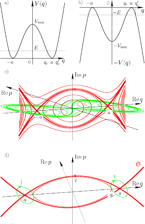
Figure 1: (colour online) In the case of a double well potential shown in a), tunnelling can be described by a solution of (14) with a purely real $q$ evolving from one well to the other. In phase-space, this trajectory appears to be a concatenation of two types of curves that join on the $(\operatorname{Re}q)$-axis: 1) a trajectory that lies in the phase-space plane $(\operatorname{Re}q,\operatorname{Re}p)$ with real variations of $t$ at energy $E$ with the potential $V$ and 2) a trajectory that lies in the phase-space plane $(\operatorname{Re}q,\operatorname{Im}p)$ with imaginary variations of $t$ at energy $-E$ with the potential $-V$ shown in b). In c) a family of constant energy curves is shown (horizontal green (light gray) for the first type, vertical red (dark gray) for the second type). In d) for a given energy, we show how the three curves $\mathfrak{l},\mathfrak{c},\mathfrak{r}$ glue together at the turning points $(0,\pm q_{r})$. $\mathfrak{S}$ denotes the separatrix $\operatorname{Im}p=\pm\sqrt{2V(q)}$.

Before we make any semiclassical approximations, we check in Fig. 2 the validity of the estimation (9) on the quartic potential by a) verifying that $\Delta_{0}(T)$ is almost real and independent of the choice of the complex $T$ provided that conditions (6) and (8) are fulfilled, and b) by checking that this constant gives a good approximation of the “exact” $\Delta E_{0}$ computed by direct numerical diagonalization of the Hamiltonian Korsch/Gluck02a .

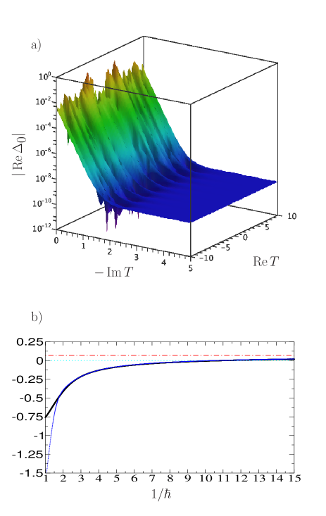
Figure 2: (colour online) For $V(q)=(q^{2}-a^{2})^{2}$ with $a=1$ and $\hbar\simeq 1/12$, we have plotted in the upper graph a) the real part of $\Delta_{0}$ defined by (9) as a function of the complex $T$. It becomes constant for $\operatorname{Im}T$ large enough for having (6) ($1/\omega=1/(2\sqrt{2}a)\simeq.35$) regardless of $\operatorname{Re}T$. In the same range, $\operatorname{Im}\big{(}\Delta_{0}(T))$ is negligible compared to $\Delta E_{0}\sim 4.4\;10^{-10}$ and condition (8) is largely fulfilled. In the lower graph b), we have computed the “exact” value $\Delta E_{0}$ by direct diagonalization. The black thick solid line corresponds to $\ln(\Delta E_{0})$ from which we have substracted $\Lambda(\hbar)\;\smash{\overset{\text{\tiny def}}{=}}-\tilde{S}_{\mathfrak{c}}(\hbar\omega/2)/(2\hbar)+\ln(\hbar\omega/\pi)$ in order to emphasize the contribution of the prefactor. The blue solid line corresponds to $\ln|\Delta_{0}|-\Lambda(\hbar)$ for $T\simeq-4{\mathrm{i}}$ and become indistinguishable from the previous one for $1/\hbar\gtrsim 3$. With the same substraction, our first proposal (39) gives the constant $(\ln\sqrt{\pi})\simeq 0.6$ and our second one (44), which is the same as the formula in Landau and Lifshitz (Landau/Lifshitz77a, , sec. 50, problem 3), corresponds to $0$ (dotted line). Garg’s formula (Garg00a, , eq.1.1) gives the constant $(\ln\sqrt{\pi/\mathrm{e}}\simeq 0.07)$ (dash-dotted line).

As explained at the end of section sec. III, in phase-space we will try to find some time-path $[t]$ that allows the existence a (half) symmetric periodic orbit $\mathfrak{o}$ that connects two tori at (real) energy $E\gtrsim 0$ in the neighbourhood of $(p,q)=(0,\pm a)$ while $q$ remains real. If we impose $t(s_{i})=0$ and $t(s_{f})=T$, then $E=E_{\mathfrak{o}}(q_{f},q_{i},T)$ is implicitly given by relation (83). We will denote by $q_{r}(E)$ (resp. $q^{\prime}_{r}(E)$) the position of the turning point at energy $E>0$ that lies in between $q=0$ and $q=a$ (resp. that is larger that $a$). The two branches $p_{\pm}(q,E)=\pm\sqrt{2\smash{\big{(}}E-V(q)\smash{\big{)}}}$ are either purely real when $V(q)\geqslant E$ or purely imaginary when $V(q)\leqslant E$. Then, from equation (14b),

$$\frac{\mathrm{d}t}{\mathrm{d}s}=\frac{1}{p}\,\frac{\mathrm{d}q}{\mathrm{d}s}$$ (21)

is purely real in the classically allowed region, while purely imaginary in the forbidden region. Therefore the complex time path $[t]$ must have the shape of a descending staircase whose steps are made of pure real or pure imaginary variations of time (see Fig. 3).

The complex orbit with real $q$ can be represented in phase-space as a continuous concatenation of paths, following the lines $E=(\operatorname{Re}p)^{2}/2+V\big{(}q)$ in the allowed region and $-E=(\operatorname{Im}p)^{2}/2-V(q)$ in the forbidden region. It is natural to represent $\mathfrak{o}$ in the three dimensional section $\operatorname{Im}q=0$ of the complex phase-space with axes given by $(\operatorname{Re}q,\operatorname{Re}p,\operatorname{Im}p)$: the junctions at the turning points lie necessarily on the $(\operatorname{Re}p=0,\operatorname{Im}p=0)$ axis (see Figs. 1c and d). A periodic orbit is made of a succession of repetitions of
(i) primitive real periodic orbits $\mathfrak{r}$ with energy $E$ in the right region, that is, such that $q_{r}(E)\leqslant q(s)\leqslant q_{r}^{\prime}(E)$ and $\operatorname{Im}p(s)=0$;
(ii) primitive complex periodic orbits $\mathfrak{c}$ in the central region with purely imaginary $p$ and real $q$, that is, such that $-q_{r}(E)\leqslant q(s)\leqslant q_{r}(E)$ and $\operatorname{Re}p(s)=0$;
(iii) primitive real periodic orbits $\mathfrak{l}$ with energy $E$ in the left region. They are obtained from the periodic orbits $\mathfrak{r}$ by the symmetry $\mathsf{S}$.

By denoting $T_{\mathfrak{r}}(E)$ and $T_{\mathfrak{c}}(E)$ the (real, positive) periods of the primitive periodic orbits $\mathfrak{r}$ and $\mathfrak{c}$ at energy $E$ respectively, we have

$$T_{\mathfrak{o}}(E)=w_{\mathfrak{r}}T_{\mathfrak{r}}(E)-{\mathrm{i}}w_{\mathfrak{c}}T_{\mathfrak{c}}(E)-{\mathrm{i}}\frac{1-\eta}{4}\,T_{\mathfrak{c}}(E)$$ (22)

with the winding numbers $w_{\mathfrak{r}}$ and $w_{\mathfrak{c}}$ being non-negative integers. The trajectory $\mathfrak{o}$ may contribute to the denominator ($\eta=+1$) or to the numerator ($\eta=-1$) of the right hand side of (9) provided that $T_{\mathfrak{o}}=T$. For $\eta=+1$, $\mathfrak{o}$ is periodic whereas, for $\eta=-1$, $\mathfrak{o}$ is half a symmetric periodic orbit. We will keep the contributions of all orbits for which a staircase $[t]$ can be constructed. We can understand from figure 3 that orbits differing by a small sliding of their initial $q_{i}$ can be obtained by a small modification of the length or height of the first step. All these contributions are summed up when performing the integral (17) on one branch $\beta$ and correspond to one term in the sum $\sum_{\beta}$ in formula (19b). When at least one of the winding number is strictly larger than one, several staircase time-paths can be constructed while keeping relation (22): they differ one from each other by a different partition into steps of the length and/or heights of the staircase. The corresponding orbits $\mathfrak{o}$ can be obtained one from each other by a continuous smooth sliding of the steps of the staircase but during this process one cannot avoid an orbit starting at a turning point where a bifurcation occurs.

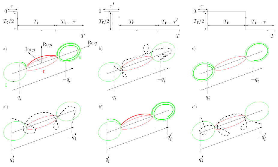
Figure 3: (colour online) For the double well in Fig. 1, at a given energy $0<E<V_{\mathrm{max}}$, when $T=2T_{\mathfrak{r}}(E)-{\mathrm{i}}T_{\mathfrak{c}}(E)/2$, for each one-step time path, there exists a unique half symmetric periodic orbit with energy $E$ keeping $\operatorname{Im}q=0$ starting from the left allowed region. Its initial point is uniquely defined: For the time-path depicted in the left column, $(p_{i},q_{i})$ is such that it takes exactly the real time $\tau$ to reach the turning point $(0,-q_{r})$ following the primitive orbit $\mathfrak{l}$. Then it follows half of the orbit $\mathfrak{c}$ and ends in the right well winding once along $\mathfrak{r}$ (a). When starting at $q_{i}^{\prime}<q_{i}$, there still exists a half periodic orbit joining $(p^{\prime}_{i},q^{\prime}_{i})$ to $(-p^{\prime}_{i},-q^{\prime}_{i})$ in time $T$ for some $p^{\prime}_{i}$ but unlike the previous one it gets outside the three dimensional section $\operatorname{Im}q=0$ (its projection is schematically represented by the dashed line in a’). However an appropriate shift of the time step to $\tau^{\prime}>\tau$ (central column) turns the latter smoothly into a trajectory with $\operatorname{Im}q=0$ (b’). During this process, the first trajectory starting at $q_{i}$ cannot keep a purely real $q$ anymore (b). If we shift the step by exactly $T_{\mathfrak{r}}$ (right column), we recover a trajectory starting at $q_{i}$ with purely real $q$ (c) but with a different topology since it is now winding once along $\mathfrak{l}$. The change of topology occurs when the initial position reaches a turning point while sliding the step.

In the right hand side of (16), the sum involves several trajectories differing one from each other by the sequence of turning points that are successively encountered along $\mathfrak{o}$. Therefore, to compute the dominant contribution of the non-zero length orbits to the numerator and to the denominator of (9), we will add all the contributions of the topological classes of orbits, each of them uniquely characterised by an ordered sequence of turning points $[\rho_{1},\rho_{2},\dots]$, in other words by a partition of $w_{\mathfrak{r}}$ and $w_{\mathfrak{c}}$ into integers and by the branch $\beta$ where its starting point lies. We can therefore express our result in a way that can be applied to cases more general than the double well: the total contribution of the non-zero length paths to the numerator ($\eta=-1$) and to the denominator ($\eta=+1$) of (9) is

$$\sum_{\mathfrak{s}}\sum_{[\rho_{1},\rho_{2},\dots]}(-1)^{\mu_{\mathfrak{o}}}\frac{T_{\beta}}{\sqrt{-2\eta{\mathrm{i}}\pi\hbar}}\sqrt{\frac{\mathrm{d}E_{\mathfrak{o}}}{\mathrm{d}T}}\;\mathrm{e}^{{\mathrm{i}}S_{\mathfrak{o}}/\hbar}\;.$$ (23)

$\mathfrak{s}$ denotes a section of an energy surface in complex phase space corresponding to one purely real canonical variable. $[\rho_{1},\rho_{2},\dots]$ is an ordered sequence of (not necessarily distinct) turning points that belong to a section $\mathfrak{s}$. The sum concerns all $\mathfrak{s}$ (different energies may be possible) and $[\rho_{1},\rho_{2},\dots]$ such that we can construct on $\mathfrak{s}$, with an appropriate choice of $[t]$, a periodic orbit $\mathfrak{o}$ if $\eta=+1$ (a half symmetric periodic orbit $\mathfrak{o}$ if $\eta=-1$) of period $T_{\mathfrak{o}}=T$. The branch $\beta$ is the one where $\mathfrak{o}$ starts, the sequence of turning points that are successively crossed by $\mathfrak{o}$ is exactly $[\rho_{1},\rho_{2},\dots]$.

In the case of the double-well, for an energy below $V_{\mathrm{max}}$, a section $\mathfrak{s}$ for real $q$ has four turning points $(0,\pm q_{r})$ and $(0,\pm q^{\prime}_{r})$. Only the points on $\mathfrak{s}$ such that $-q^{\prime}_{r}<q<q^{\prime}_{r}$ can provide starting points of a periodic orbit. They belong to one of the three closed loops $\mathfrak{r}$,$\mathfrak{c}$, $\mathfrak{l}$ that connect on the axis $(p=0,\operatorname{Im}q=0)$ at the turning points $(0,\pm q_{r})$. Once $T$ is given, the condition $T_{\mathfrak{o}}=T$ will select a finite set of energies for which we have (22) with integers $w_{\mathfrak{r}}$ and $w_{\mathfrak{c}}$. Any $\mathfrak{o}$ with winding numbers $w_{\mathfrak{r}}$ and $w_{\mathfrak{c}}$ will have an action given by

$$S_{\mathfrak{o}}=w_{\mathfrak{r}}S_{\mathfrak{r}}+{\mathrm{i}}w_{\mathfrak{c}}S_{\mathfrak{c}}+{\mathrm{i}}\frac{1-\eta}{4}\,S_{\mathfrak{c}}$$ (24)

and an index

$$\mu_{\mathfrak{o}}=w_{\mathfrak{r}}+w_{\mathfrak{c}}+\frac{1-\eta}{2}$$ (25)

(in the real case, $2\mu_{\mathfrak{o}}$ is computed in the same way as the Maslov index: it counts the number of turning points encountered along $\mathfrak{o}$). These quantities are independent on the choice of the six possible starting branch $\beta$ (each $\mathfrak{r}$, $\mathfrak{c}$, $\mathfrak{l}$ is made of two branches). When the orbit $\mathfrak{o}$ starts on $\mathfrak{r}$ or on $\mathfrak{l}$, we will have $T_{\beta}=T_{\mathfrak{r}}/2$ and when $\mathfrak{o}$ starts on $\mathfrak{c}$, we have $T_{\beta}=-{\mathrm{i}}T_{\mathfrak{c}}/2$.

For $-\operatorname{Im}T$ larger than the oscillation period in the central well of $-V$, $w_{\mathfrak{c}}=1$ is the minimum value of the winding number when $\eta=+1$ (just one back and forth trip around $\mathfrak{c}$) while it is $w_{\mathfrak{c}}=0$ when $\eta=-1$ (just one half of $\mathfrak{c}$ is concerned). For these orbits, condition (6) forces $\mathfrak{c}$ to stay near the separatrix $\mathfrak{S}$ defined by $\operatorname{Im}p=\pm\sqrt{2V(q)}$ and, thus, $\mathfrak{r}$ must lie in the immediate neighbourhood of the equilibrium point $(p,q)=(0,a)$. These orbits will give the dominant contribution because they have the smallest $\operatorname{Im}S_{\mathfrak{o}}$ among all the other possible orbits involving repetitions of $\mathfrak{c}$. Indeed, for a fixed $T$, all the orbits $\mathfrak{o}$ that may contribute semiclassically are such that $\operatorname{Im}S_{\mathfrak{o}}=-2\operatorname{Im}(T)S_{\mathfrak{c}}/T_{\mathfrak{c}}$ and $S_{\mathfrak{c}}/T_{\mathfrak{c}}$ is a decreasing function of the energy $\tilde{E}\;\smash{\overset{\text{\tiny def}}{=}}-E$ when $\mathfrak{c}$ is inside the separatrix since

$$\frac{\mathrm{d}}{\mathrm{d}\tilde{E}}\left(\frac{S_{\mathfrak{c}}(\tilde{E})}{T_{\mathfrak{c}}(\tilde{E})}\right)=\\ \frac{\mathrm{d}}{\mathrm{d}\tilde{E}}\left(\frac{4}{T_{\mathfrak{c}}(\tilde{E})}\int_{0}^{q_{r}(-\tilde{E})}\sqrt{2\big{(}\tilde{E}+V(q)\big{)}}\mathrm{d}q-\tilde{E}\right)\\ =-\frac{4}{T_{\mathfrak{c}}(\tilde{E})^{2}}\frac{\mathrm{d}T_{\mathfrak{c}}(\tilde{E})}{\mathrm{d}\tilde{E}}\int_{0}^{q_{r}(E)}|p(q,E)|\mathrm{d}q<0\;.$$ (26)

Therefore $\operatorname{Im}S_{\mathfrak{o}}$ reaches its minimum when $\tilde{E}$ is at its maximum, that is $E\to 0^{+}$. The only possible equilibrium point contributing to $\operatorname*{tr}\!\big{(}\hat{\mathsf{S}}\,\hat{U}(T)\big{)}$ is the origin $(p_{f},q_{f})=(-p_{i},q_{i})=(0,0)$; it is also subdominant because $H(0,0)=V(0)=V_{\textrm{max}}$ (which can be seen as the limit of $S_{\mathfrak{c}}(\tilde{E})/T_{\mathfrak{c}}(\tilde{E})$ when $\tilde{E}\to-V_{\textrm{max}}$) is strictly larger than $S_{\mathfrak{c}}(\tilde{E})/T_{\mathfrak{c}}(\tilde{E})$ for $\tilde{E}>-V_{\textrm{max}}$.

Assuming that only orbits with real $q$ do contribute to $\operatorname*{tr}\!\big{(}\hat{\mathsf{S}}\,\hat{U}(T)\big{)}$, we have proven that the dominant contribution is given by the half symmetric orbits $\mathfrak{o}$ at energy $E$ such that $T_{\mathfrak{c}}(E)=-2\operatorname{Im}T$ ($w_{\mathfrak{c}}=0$). However, for such an orbit to exist we cannot choose $\operatorname{Re}T$ arbitrarily since it must be an integer multiple of $T_{\mathfrak{r}}(E)$. To put it in another way, for a given $E$, we will choose $T=w_{\mathfrak{r}}T_{\mathfrak{r}}(E)-{\mathrm{i}}T_{\mathfrak{c}}(E)/2$ such that an orbit $\mathfrak{o}$ with a real $q$ exists. Condition (6) will be fulfilled if $E$ is sufficiently small. We must now enumerate all the topological classes concerned by the sum (23): When $\mathfrak{o}$ starts on the upper branch $\operatorname{Im}p>0$ of $\mathfrak{c}$, it will reach the turning point $\rho_{1}=(0,q_{r})$ then wind $w_{\mathfrak{r}}$ times around $\mathfrak{r}$ alternatively crossing $(0,q_{r}^{\prime})$ and $(0,q_{r})$ before turning back on the lower branch $\operatorname{Im}p<0$ of $\mathfrak{c}$. Starting on the lower branch of $\mathfrak{c}$ corresponds to the symmetric trajectory and provide the same contribution with $T_{\beta}=-{\mathrm{i}}T_{\mathfrak{c}}/2$. When starting on the upper branch of $\mathfrak{r}$, $\mathfrak{o}$ crosses $\rho_{1}=(0,q^{\prime}_{r})$ first, then reaches $\rho_{2}=(0,q_{r})$. Then it may go on winding $r$ times around $\mathfrak{r}$ then take the lower branch of $\mathfrak{c}$ up to the turning point $(0,-q_{r})$, wind $w_{\mathfrak{r}}-1-r$ times around $\mathfrak{l}$ and eventually join the symmetric of its starting point on the lower branch of $\mathfrak{l}$. There are exactly $w_{\mathfrak{r}}$ such topological classes because we can take $r=0,...,w_{\mathfrak{r}}-1$. If we start from the lower branch of $\mathfrak{r}$ or on one of the two branches of $\mathfrak{l}$, we obtain the same contribution and exhaust the possible topological classes. The sum of $T_{\beta}$ on all $\beta$’s and classes is then $2(-{\mathrm{i}}T_{\mathfrak{c}}/2)+4w_{\mathfrak{r}}T_{\mathfrak{r}}/2=2T$ and keeping only the $w_{\mathfrak{c}}=0$ solutions, the sum (23) reduces to

$$\operatorname*{tr}\!\big{(}\hat{\mathsf{S}}\,\hat{U}(T)\big{)}\underset{\hbar\to 0}{\sim}\frac{2T(-1)^{w_{\mathfrak{r}}+1}}{\sqrt{2{\mathrm{i}}\pi\hbar}}\sqrt{\frac{\mathrm{d}E_{\mathfrak{o}}}{\mathrm{d}T}}\;\text{\Large e}^{{\mathrm{i}}S_{\mathfrak{o}}/\hbar}$$ (27)

with $\mathfrak{o}$ being one half symmetric orbit of energy $E_{\mathfrak{o}}$ defined implicitly by

$$T=w_{\mathfrak{r}}T_{\mathfrak{r}}(E)-{\mathrm{i}}T_{\mathfrak{c}}(E)/2$$ (28)

with

$$T_{\mathfrak{r}}(E) =2\int_{q_{r}(E)}^{q^{\prime}_{r}(E)}\frac{\mathrm{d}q}{\sqrt{2\big{(}E-V(q)\big{)}}}\;,$$ (29a)

$$T_{\mathfrak{c}}(E) =4\int_{0}^{q_{r}(E)}\frac{\mathrm{d}q}{\sqrt{2\big{(}V(q)-E\big{)}}}\;.$$ (29b)

We have $S_{\mathfrak{o}}(E)=w_{\mathfrak{r}}S_{\mathfrak{r}}(E)+{\mathrm{i}}S_{\mathfrak{c}}(E)/2$ with

$$S_{\mathfrak{r}}(E)+ET_{\mathfrak{r}}(E) =\tilde{S}_{\mathfrak{r}}(E)\overset{\mathrm{def}}{=}2\int_{q_{r}(E)}^{q^{\prime}_{r}(E)}\!\!\sqrt{2\big{(}E-V(q)\big{)}}\,\mathrm{d}q,$$ (30a)

$$\vspace{-2\baselineskip}S_{\mathfrak{c}}(E)-ET_{\mathfrak{c}}(E) =\tilde{S}_{\mathfrak{c}}(E)\overset{\mathrm{def}}{=}4\int_{0}^{q_{r}(E)}\!\!\sqrt{2\big{(}V(q)-E\big{)}}\,\mathrm{d}q.$$ (30b)

The dominant contributions to $\operatorname*{tr}\!\big{(}\hat{U}(T)\big{)}$ comes from the two stable equilibrium points $\mathfrak{e}=(0,\pm a)$ for which $\lambda_{\mathfrak{e}}={\mathrm{i}}\omega$. The contribution of $(0,0)$ is sub-dominant as well as the contribution of any periodic orbit $\mathfrak{o}$ which necessarily turns around about $\mathfrak{e}$ during $\operatorname{Re}T$ then follow an orbit $\mathfrak{c}$ near $\mathfrak{S}$ during $-\operatorname{Im}T$ before coming back to its initial point. Together with (6), $\eta=1$, the two stable equilibrium points give two identical contributions (19a) and we have

$$\operatorname*{tr}\!\big{(}\hat{U}(T)\big{)}\underset{\hbar\to 0}{\sim}2\,\mathrm{e}^{-{\mathrm{i}}\omega T/2}$$ (31)

which of course could have been deduced directly from $E_{0}^{\pm}\simeq\hbar\omega/2$. Collecting all these results in the right hand side of (9), we obtain

$$\Delta_{0}\underset{\hbar\to 0}{\sim}\sqrt{\frac{2{\mathrm{i}}\hbar}{\pi}}\left(\frac{\mathrm{d}T_{\mathfrak{o}}}{\mathrm{d}E}\right)^{-1/2}\\ \times\exp{\left(-\frac{1}{2\hbar}\Big{(}\tilde{S}_{\mathfrak{c}}(E)+(E-\hbar\omega/2)T_{\mathfrak{c}}(E)\Big{)}\right)}\\ \times\,\exp{\left(\frac{{\mathrm{i}}w_{\mathfrak{r}}}{\hbar}\Big{(}\tilde{S}_{\mathfrak{r}}(E)-(E-\hbar\omega/2)T_{\mathfrak{r}}(E)-\hbar\pi\Big{)}\right)}.$$ (32)

When $E\to 0^{+}$, we have the following asymptotic expansions (see appendix B)

$$\tilde{S}_{\mathfrak{c}}(E) =\tilde{S}_{\mathfrak{c}}(0)+\frac{4E}{\omega}\ln\bigg{(}\frac{\sqrt{2E}}{2a\omega}\bigg{)}-\frac{2(2A+1)}{\omega}E+\mathrm{o}(E)\;;$$ (33a)

$$\tilde{S}_{\mathfrak{r}}(E) =\frac{2\pi E}{\omega}+BE^{2}+\mathrm{o}(E^{2})\;;$$ (33b)

with

$$A \overset{\mathrm{def}}{=}\int_{0}^{a}\left(\frac{\omega}{\sqrt{2V(q)}}-\frac{1}{a-q}\right)\,\mathrm{d}q\;;$$ (34)

$$B \overset{\mathrm{def}}{=}\frac{\pi}{24\omega^{7}}\big{(}5V^{(3)}(a)^{2}-3\omega^{2}V^{(4)}(a)\big{)}$$ (35)

(the superscript in parenthesis indicates the order of the derivative of $V$). The differentiation of expressions (33) with respect to $E$ leads to the asymptotic expansions for $-T_{\mathfrak{c}}$ and $T_{\mathfrak{r}}$. From the first one we can extract the exponential sensitivity of $E$ on $\operatorname{Im}T$:

$$E\simeq 2a^{2}\omega^{2}\mathrm{e}^{2A}\mathrm{e}^{\omega\operatorname{Im}T}\;.$$ (36)

From relation (28) we can see that $2\mathrm{d}T_{\mathfrak{o}}/\mathrm{d}E=2w_{\mathfrak{r}}\,\mathrm{d}T_{\mathfrak{r}}/\mathrm{d}E-{\mathrm{i}}\,\mathrm{d}T_{\mathfrak{c}}/\mathrm{d}E$ is dominated by the last term if $E$ is small.

$$\frac{\mathrm{d}T_{\mathfrak{o}}}{\mathrm{d}E}\simeq-\frac{{\mathrm{i}}}{2}\,\frac{\mathrm{d}T_{\mathfrak{c}}}{\mathrm{d}E}\simeq\frac{{\mathrm{i}}}{\omega E}\;.$$ (37)

Inserting all these asymptotic expansions in the right hand side of (32), we get

$$\Delta_{0}\underset{\hbar\to 0}{\sim}\sqrt{\frac{4\hbar a^{2}\omega^{3}}{\pi}}\mathrm{e}^{A}\mathrm{e}^{E/(\hbar\omega)}\,\mathrm{e}^{-\tilde{S}_{\mathfrak{c}}(0)/(2\hbar)}\\ \times\mathrm{e}^{-{\mathrm{i}}w_{\mathfrak{r}}BE(E-\hbar\omega)/\hbar}\;.$$ (38)

This expression can be turned into the usual jwkb expansion $\exp\big{(}a_{0}(E)/\hbar+a_{1}(E)\ln\hbar+a_{2}(E)+\mathrm{o}(1)\big{)}$: As soon as we have condition (6), from expression (36) we see that $E$ is exponentially small and we obtain $a_{0}(0)=-\tilde{S}_{\mathfrak{c}}(0)/2$ and $a_{1}(0)=1/2$. To obtain the correct value of $a_{2}$, we must proceed to fine-tune the choice of $T$. A criterion is to impose on $\Delta_{0}$ to have a vanishing imaginary part at any order in $\hbar$ consistent with the jwkb expansions used so far. From (32), we will choose $E$ such that $\tilde{S}_{\mathfrak{r}}(E)=\hbar\pi$, which is exactly the Einstein-Brillouin-Keller quantization condition for the ground state in one well. This leads to $E=\hbar\omega/2+\mathrm{o}(\hbar)$. Then $T_{\mathfrak{c}}=-2\ln\big{(}\hbar/(4a^{2}\omega)\big{)}/\omega+4A/\omega+\mathrm{o}(1)$ and

$$\Delta_{0}\underset{\hbar\to 0}{\sim}\frac{\hbar\omega}{\sqrt{\pi}}\mathrm{e}^{-\tilde{S}_{\mathfrak{c}}(\hbar\omega/2)/(2\hbar)}=2a\omega\sqrt{\frac{\mathrm{e}\hbar\omega}{\pi}}\mathrm{e}^{A}\mathrm{e}^{-\tilde{S}_{\mathfrak{c}}(0)/(2\hbar)},$$ (39)

which differs from (Garg00a, , eqs. (1.1) and (1.4)) by a reasonable factor $\sqrt{\mathrm{e}}\simeq 1.6$. This discrepancy, already noticed in (Gildener/Patrascioiu77a, , sec. V), which appears in the third order term in the $\hbar$-expansion, comes from the different kind of approximations involved in our approach on the one hand and in Herring’s formula on the other hand.

We are also able to obtain a formula for the splitting of the excited states that is consistent with the result given in (Garg00a, , eq. (B1)). Using a semiclassical approximation for the matrix element of $\hat{\varPi}_{n}$, we explain in detail in appendix C how to obtain $\Delta_{n}(T)$. For one dimensional systems whose energy surface $E_{n}$ is made of two branches (two Riemann sheets in the complex plane), we can insert (103) into (101) and get one of the main result of this paper:

$$\Delta_{n}(T)\underset{\hbar\to 0}{\sim}\frac{\hbar}{2T}\sum_{[\rho_{1},\rho_{2},\dots]}(-1)^{\mu_{\mathfrak{o}}+1}\mathrm{e}^{{\mathrm{i}}\tilde{S}_{\mathfrak{o}}(b_{\beta^{\prime}},b_{\beta},E_{n})/\hbar}\;.$$ (40)

To see how formula (40) works in the case of the double-well potential, we choose the quasi-mode $\mathinner{|{\Phi_{n}}\rangle}$ localised on the right torus $\mathfrak{r}$ at energy $E_{n}$. This torus is made of two branches labelled by the sign of $p$ and we can choose a common base point for these two branches, namely $b_{\pm}=q_{r}(E)$. On the symmetric torus $\mathfrak{l}$, the two base points will be $b_{\pm}=-q_{r}(E)$. Then $\tilde{S}_{\mathfrak{o}}(b_{\beta^{\prime}},b_{\beta},E_{n})$ and the index $\mu_{\mathfrak{o}}$ do not depend on the choice of the initial and final branch. The orbits $\mathfrak{o}$ that go from $\mathfrak{r}$ to $\mathfrak{l}$ must correspond to a $T$ of the form

$$T=\tau+w_{\mathfrak{r}}T_{\mathfrak{r}}(E_{n})-{\mathrm{i}}\left(w_{\mathfrak{c}}+\frac{1}{2}\right)T_{\mathfrak{c}}(E_{n})$$ (41)

for non-negative integer $(w_{\mathfrak{c}},w_{\mathfrak{r}})$ and a fraction of time $\tau$ strictly smaller that $T_{\mathfrak{c}}(E_{n})$ that depends on the initial and final conditions (those are not necessarily symmetric). Then we have

$$\tilde{S}_{\mathfrak{o}}(b_{\beta^{\prime}},b_{\beta},E_{n})=w_{\mathfrak{r}}\tilde{S}_{\mathfrak{r}}(E_{n})+{\mathrm{i}}\left(w_{\mathfrak{c}}+\frac{1}{2}\right)\tilde{S}_{\mathfrak{c}}(E_{n})$$ (42)

and we take

$$\mu_{\mathfrak{o}}=w_{\mathfrak{r}}+w_{\mathfrak{c}}+1\;.$$ (43)

For the same reason as previously explained the dominant contributions come from those orbits where $w_{\mathfrak{c}}=0$. In order to mimic a real $T$, we will choose large winding numbers $w_{\mathfrak{r}}$ such that $\operatorname{Re}T=w_{\mathfrak{r}}T_{\mathfrak{r}}(E_{n})\gg\operatorname{Im}T=T_{\mathfrak{c}}(E_{n})/2$. Because of the quantization condition in the right well $\tilde{S}_{\mathfrak{r}}(E_{n})=(n+1/2)2\pi\hbar$, the rapid oscillations $\exp({\mathrm{i}}\operatorname{Re}S_{\mathfrak{o}}/\hbar)$ disappear (or inversely if we want to maintain $\Delta_{n}$ real to first order, we recover the usual quantization condition). Then we obtain

$$\Delta_{n}\underset{\hbar\to 0}{\sim}\frac{2\hbar}{T_{\mathfrak{r}}(E_{n})}\,\mathrm{e}^{-\tilde{S}_{\mathfrak{c}}(E_{n})/(2\hbar)}\;.$$ (44)

The classical frequency $1/T_{\mathfrak{r}}(E_{n})$ attached to $\mathfrak{r}$ is essentially of order $\omega/(2\pi)$. $\Delta_{n}(T)$ becomes independent of $T$ for large $w_{\mathfrak{r}}$: the behaviour of $T$ is mainly governed by $w_{\mathfrak{r}}T_{\mathfrak{r}}$, then the $1/T$ prefactor in (40) is compensated by the increasing number of identical terms in the sum since we have seen that the number of topological classes of orbits increases linearly with $4w_{\mathfrak{r}}$ (the factor 4 comes from the two possible initial branches $\beta=\pm$ and the two possible final branches $\beta^{\prime}=\pm$; in other words from the sequences of $[\rho_{1},\rho_{2},\dots]$ beginning either by $q_{r}$ or $q_{r}^{\prime}$ and ending either by $-q_{r}$ or $-q_{r}^{\prime}$). The discrepancy between (44) and Garg’s formula is just the factor $g_{n}$ given by (Garg00a, , eq. (B2)) (see also(Connor+84a, , eq. (3.41))) that tends to 1 when $n$ increases: $g_{0}=\sqrt{\pi/\mathrm{e}}\simeq 1.075$, $g_{1}\simeq 1.028$, …There is also a ratio of order one, more precisely $\sqrt{2/\pi}\simeq 0.8$, between estimations (39) and (44) taken for $n=0$; the second is slightly better and coincides with the formula given in Landau and Lifshitz (Landau/Lifshitz77a, , sec. 50, problem 3). Again, these discrepancies come from the different nature of the approximations that are involved.

Let us end this section by a short comment on the connection with the usual instanton theory where $\operatorname{Re}T=0$ and where $\operatorname{Im}T\to-\infty$. This regime, that allows to select the ground-state doublet only, is included in our approach because the instanton trajectories appear to be the limit of $\mathfrak{c}$ getting closer to the separatrix $\mathfrak{S}$ whereas the classical real oscillations in the wells shrink to the equilibrium points. All along this paper we emphasize that the phase-space representation is particularly appropriate and it is straightforward to recover the usual picture of instantons (for instance $q({\mathrm{i}}t)$ versus ${\mathrm{i}}t$) from our figure 1 d).

V Dynamical tunnelling for the simple pendulum

The simple pendulum corresponds to $V(q)=-\gamma\cos q$ with $\gamma>0$ and strictly periodic boundary conditions that identify $q=-\pi$ and $q=\pi$. At energy $E>\gamma$, the classical rotation with $p=\sqrt{2(E-V(q))}$ can never switch to the inverse rotation with $-p=-\sqrt{2(E-V(q))}$. At the quantum level, the Schrödinger’s equation for the stationary wave-function $\phi$

$$\left[-\frac{\hbar^{2}}{2}\frac{\mathrm{d}^{2}}{\mathrm{d}q^{2}}-\gamma\cos q\right]\phi(q)=E\phi(q)$$ (45)

leads to the Mathieu equation Abramowitz/Segun65a ,

$$y^{\prime\prime}(x)+\big{(}a-2g\cos(2x)\big{)}y(x)=0$$ (46)

with $x=q/2$, $y(x)=\phi(2x)$, $a=8E/\hbar^{2}$ and $g=-4\gamma/\hbar^{2}$. The $2\pi$-periodicity of $\phi$ forces $y$ to be $\pi$-periodic. The eigenfunctions can be classified according to the parity operator: Even $\pi$-periodic solutions exist only for a countably infinite set of characteristic values of $a$ denoted by $\{a_{2n}\}$ with $n=0,1,\dots$ Odd solutions correspond to another set, $\{b_{2n}\}$, with $n=1,2\dots$ (the $\{a_{2n+1},b_{2n+1}\}$ correspond to $\pi$-antiperiodic solutions and will be rejected). The discrete energy spectrum corresponding to even and odd solutions of (45) is then $\{E^{+}_{n}=\hbar^{2}a_{2n}/8,n=0,1\dots\}$ and $\{E^{-}_{n}=\hbar^{2}b_{2n}/8,n=1,2\dots\}$ respectively. Any eigenstate $\mathinner{|{\phi_{n}^{\pm}}\rangle}$ with energy $E^{\pm}_{n}\simeq E_{n}>\gamma$ has its Husimi distribution spread symmetrically between the two half phase-space of positive and negative $p$, near the lines $\pm\sqrt{2(E_{n}-V(q))}$ that define two disconnected tori in the cylindrical phase-space. If we prepare a wave-packet localised on the line $p=\sqrt{2(E_{n}-V(q))}$, since it is no longer a stationary state, its average momentum will oscillate between two opposite values, with a tunnelling frequency equal to $\Delta E_{n}/\hbar$ where

$$\Delta E_{n}=E^{+}_{n}-E^{-}_{n}=\frac{\hbar^{2}}{8}(a_{2n}-b_{2n})$$ (47)

is the splitting between the two quasi-degenerate eigenenergies. To compute $\Delta E_{n}$, we will use (10) with the operator $\hat{\varPi}_{n}$ very much like the exact projector $\mathinner{|{\phi_{n}^{+}}\rangle}\mathinner{\langle{\phi_{n}^{+}}|}+\mathinner{|{\phi_{n}^{-}}\rangle}\mathinner{\langle{\phi_{n}^{-}}|}$: Its matrix element $\mathinner{\langle{p^{\prime}}|}\hat{\varPi}_{n}\mathinner{|{p}\rangle}$ will vanish rapidly as soon as $p$ or $p^{\prime}$ lie outside the region of the two tori. The main contribution to the semiclassical expansion of $\operatorname*{tr}\!\big{(}\hat{\mathsf{S}}\,\hat{\varPi}_{n}\,\hat{U}(T)\big{)}$ will come from classical trajectories that connect two symmetric tori. The trace will be semiclassically computed in the momentum basis and we will choose the complex time path to maintain $p$ real. To construct one trajectory at energy $E>\gamma$ connecting the two tori requires to have purely imaginary $q$ whenever $-p_{r}<p<p_{r}$ with $p_{r}\;\smash{\overset{\text{\tiny def}}{=}}\sqrt{2(E-\gamma)}$ being the classical turning point in momentum. More precisely, $q$ is given by $\cos q=-1-(p_{r}^{2}-p^{2})/(2\gamma)$. From (14a)

$$\frac{\mathrm{d}t}{\mathrm{d}s}=-\frac{1}{\gamma\sin q}\frac{\mathrm{d}p}{\mathrm{d}s}\,$$ (48)

we see immediately that $\sin\big{(}q(s)\big{)}$ and $\mathrm{d}t/\mathrm{d}s$ will be real when $p(s)>p_{r}$ or $p(s)<-p_{r}$ and purely imaginary otherwise. In the latter case, since we keep $p_{2}(s)\;\smash{\overset{\text{\tiny def}}{=}}\operatorname{Im}p(s)=0$, equations (15b,c) lead to two possible families of solutions (i) $q_{1}(s)\;\smash{\overset{\text{\tiny def}}{=}}\operatorname{Re}q(s)=0$ and (ii) $q_{1}(s)=\pm\pi$. Then, with $p_{1}\;\smash{\overset{\text{\tiny def}}{=}}\operatorname{Re}p$ and $q_{2}\;\smash{\overset{\text{\tiny def}}{=}}-\operatorname{Im}q$, equations (15a,d) become

$$\frac{\mathrm{d}p_{1}}{\mathrm{d}s} =\pm\gamma\operatorname{sh}q_{2}\left({\mathrm{i}}\frac{\mathrm{d}t}{\mathrm{d}s}\right)\;;$$ (49a)

$$\frac{\mathrm{d}q_{2}}{\mathrm{d}s} =p_{1}\left({\mathrm{i}}\frac{\mathrm{d}t}{\mathrm{d}s}\right)$$ (49b)

and are associated with a real time dynamics governed by the Hamiltonian

$$\tilde{H}(p_{1},q_{2})=p_{1}^{2}/2\mp\gamma\operatorname{ch}q_{2}\;.$$ (50)

with “$-$” corresponding to case (i) and “$+$” corresponding to case (ii). Then, instantons correspond to trajectories evolving in the transformed potential $\tilde{V}(q)\;\smash{\overset{\text{\tiny def}}{=}}\mp\gamma\operatorname{ch}q$ rather than the usual inverted potential $-V(q)$. We will choose a one step complex time path as in Fig. 3 and we will represent the orbits in a three dimensional space $(\operatorname{Re}q,\operatorname{Re}p,\operatorname{Im}q)$ and the connection between the allowed and the forbidden trajectories occurs on the axes $(\operatorname{Re}q=0,\operatorname{Im}q=0)$ and $(\operatorname{Re}q=\pm\pi,\operatorname{Im}q=0)$ (Fig. 4a). Trajectories in family (i) escape from the unstable point at $\operatorname{Re}p=0,\operatorname{Im}q=0$ without coming back to the plane $\operatorname{Re}p=0,\operatorname{Re}q=0$. Only orbits in family (ii) can be used to produce periodic orbits. A typical periodic orbit $\mathfrak{o}$ connecting two symmetric rotations of the pendulum is given in Fig.4b). We will choose $\-\operatorname{Im}T$ to be precisely the half period of the periodic orbit $\mathfrak{c}$ of family (ii) at energy $E_{n}$ and $\operatorname{Re}T$ to be (an integer multiple of) the period of rotation of the pendulum at the same energy. This choice exhibits the dominant contribution to $\operatorname*{tr}\!\big{(}\hat{\mathsf{S}}\,\hat{\varPi}_{n}\,\hat{U}(T)\big{)}$. We can reproduce the same reasoning that led to (44) with the rôle of $p$ and $q$ being exchanged. Now $T_{\mathfrak{r}}=\mathrm{d}\tilde{S}_{\mathfrak{r}}/\mathrm{d}E$ is the typical frequency on the torus at energy $E_{n}$.

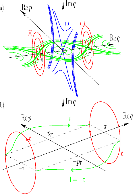
Figure 4: (colour online) With the choice of a complex-time path given in 3) (one-step path), the contributions to $\operatorname*{tr}\!\big{(}\hat{\mathsf{S}}\,\hat{\varPi}_{n}\,\hat{U}(T)\big{)}$ come from one half symmetric periodic orbits $\mathfrak{o}$ (b) that are a composite of 1) (repetitions of) a periodic orbit $\mathfrak{r}$ of period $T_{\mathfrak{r}}$ in the phase-space plane $(\operatorname{Re}q,\operatorname{Re}p)$ at energy $E>\gamma$ (recall that the planes $q=\pm\pi$ are identified); 2) one half of a periodic orbit $\mathfrak{c}$ of period $T_{\mathfrak{c}}$ in the phase-space plane $(\operatorname{Im}q,\operatorname{Re}p)$ at energy $E$.

Keeping only the contributions that provide a positive imaginary part of the action, expression (13) becomes

$$S=\int_{s_{i}}^{s_{\!f}}p_{1}(s)\frac{\mathrm{d}q_{1}}{\mathrm{d}s}(s)\mathrm{d}s-E\operatorname{Re}T\\ +{\mathrm{i}}\left(\int_{s_{i}}^{s_{\!f}}p_{1}(s)\frac{\mathrm{d}q_{2}}{\mathrm{d}s}(s)\mathrm{d}s+E(-\operatorname{Im}T)\right).$$ (51)

Then

$$S_{\mathfrak{o}}(E)=\tilde{S}_{\mathfrak{o}}(E)-ET_{\mathfrak{o}}$$ (52)

with $T_{\mathfrak{o}}=T$ and

$$\tilde{S}_{\mathfrak{o}}(E)=w_{\mathfrak{r}}\tilde{S}_{\mathfrak{r}}(E)+{\mathrm{i}}\tilde{S}_{\mathfrak{c}}(E)/2\\ =2w_{\mathfrak{r}}\int_{0}^{\pi}\sqrt{2(E+\gamma\cos q)}\,\mathrm{d}q\\ +2{\mathrm{i}}\int_{0}^{\mathrm{argch}(E/\gamma)}\sqrt{2(E-\gamma\operatorname{ch}q)}\,\mathrm{d}q\;.$$ (53)

All these expressions can be written in terms of the complete elliptic integrals Gradshteyn/Ryzhik65a (defined for $|u|<1$)

$$\mathcal{K}(u) \overset{\mathrm{def}}{=}\int_{0}^{\pi/2}\frac{\mathrm{d}x}{\sqrt{1-u^{2}\sin^{2}x}}\;;$$ (54a)

$$\mathcal{E}(u) \overset{\mathrm{def}}{=}\int_{0}^{\pi/2}\sqrt{1-u^{2}\sin^{2}x}\;\mathrm{d}x\;.$$ (54b)

Namely,

$$\tilde{S}_{\mathfrak{r}}(E) =4\sqrt{2(E+\gamma)}\,\mathcal{E}\left(\!\sqrt{\frac{2\gamma}{E+\gamma}}\,\right)\;;$$ (55a)

$$\tilde{S}_{\mathfrak{c}}(E) =8\sqrt{2(E+\gamma)}\left[\mathcal{K}\left(\!\sqrt{\frac{E-\gamma}{E+\gamma}}\,\right)-\mathcal{E}\left(\!\sqrt{\frac{E-\gamma}{E+\gamma}}\,\right)\right].$$ (55b)

Then we obtain

$$\Delta_{n}\sim\frac{2\hbar}{T_{\mathfrak{r}}(E_{n})}\,\mathrm{e}^{-\tilde{S}_{\mathfrak{c}}(E_{n})/(2\hbar)}$$ (56)

with

$$T_{\mathfrak{r}}(E)=\frac{\mathrm{d}\tilde{S}_{\mathfrak{r}}}{\mathrm{d}E}=\frac{2\sqrt{2}}{\sqrt{E+\gamma}}\,\mathcal{K}\left(\!\sqrt{\frac{2\gamma}{E+\gamma}}\,\right)\;.$$ (57)

The energies of the highly excited states are approximately given by the free rotations: $E_{n}\simeq n^{2}\hbar^{2}/2\gg\gamma$. Then $T_{\mathfrak{r}}(E_{n})\simeq 2\pi/(n\hbar)$. The asymptotic expansion of $\tilde{S}_{\mathfrak{c}}(E)$ for large $E$ leads to

$$\Delta_{n} \sim \frac{\hbar^{2}}{\pi}\frac{\sqrt{2E_{n}}}{\hbar}\;\mathrm{e}^{2(\ln(\gamma/E_{n})+2-3\ln 2)\sqrt{2E_{n}}/\hbar}\;;$$ (58a)

$$\sim \frac{1}{\pi n^{4n-1}}\left(\frac{\mathrm{e}}{2}\right)^{4n}\hbar^{2}\left(\frac{\gamma}{\hbar^{2}}\right)^{2n}\;.$$ (58b)

The last expression corresponds exactly to equation (3.44) of Connor+84a obtained with standard uniform semiclassical analysis. We see on figure 5

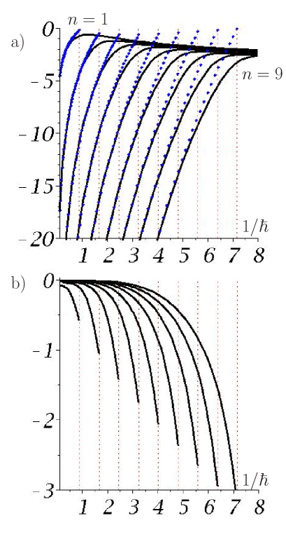
Figure 5: For the pendulum with $\gamma=1$, we have plotted in a) the exact value of $\ln(\Delta E_{n})$ (see eq. (47)) versus $1/\hbar$ for $n=1,\dots 9$ (black lines). The dots are given by the semiclassical approximation $\ln(\Delta_{n})$ (see eq. (58b)) up to the maximum value of $1/\hbar$ (vertical dotted lines) where $E_{n}^{+}$ become lower that the separatrix energy $\gamma$. The semiclassical limit is obtained when the states become more and more localised in the region of phase space corresponding to rotations: for a fixed $n$ this requires to increase $E_{n}\simeq n^{2}\hbar^{2}/2$ that is to increase $\hbar$; or for a fixed energy $E>\gamma$, we must increase $n\propto\sqrt{2E}/\hbar$. To control the validity of the prefactors, we can check in b) that $\ln(\Delta E_{n}/\Delta_{n})$ approaches zero in the semiclassical limit.

that (56) is a very good approximation even when the energies $E_{n}$ get close to $\gamma$ the energy of the separatrix.

VI Resonant tunnelling and Fabry-Pérot effect

We are now ready the see how formula (40) allows us to reproduce the resonant tunnelling between two wells related by parity when the potential in (1) has also a deeper central well (Fig. 6 a).

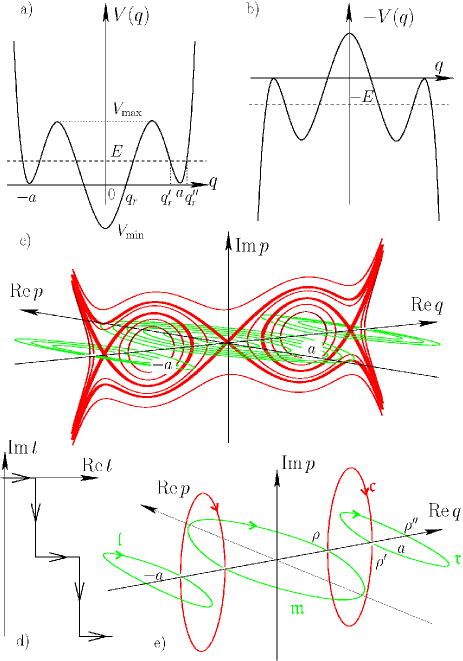
Figure 6: (colour online) To describe resonant tunnelling between two symmetric wells centered at $\pm a$ and separated by a third central well (a), we use orbits made of five primitive trajectories with a time path given in (d). We still maintain the position $q$ to be real and can use a three dimensional section of phase-space (see text). Here we have chosen $V$ given by (65) with $a=7/4$ and $b=1/2$.

The minimum of the right and left wells is fixed at zero, the minimum of the central well is $V(0)=V_{\mathrm{min}}<0$ and the local maximum between the wells is denoted $V_{\mathrm{max}}$. When $0<E<V_{\mathrm{max}}$, we will denote by $q_{r}(E)<q^{\prime}_{r}(E)<q_{r}^{\prime\prime}(E)$ the three positive solutions of $V(q)=E$. As explained in section (IV), we will try to construct appropriate time paths $[t]$ to exhibit complex trajectories $\mathfrak{o}$ with purely real $q$ that connect the two symmetric tori from $\mathfrak{r}$ to $\mathfrak{l}$ at some energy $0<E<V_{\mathrm{max}}$. These tori are delimited by the two turning points $\pm\rho^{\prime}=(0,\pm q_{r}^{\prime})$ and $\pm\rho^{\prime\prime}=(0,\pm q_{r}^{\prime\prime})$. What is new of course is the existence of a central real torus $\mathfrak{m}$ delimited by $\rho=(0,q_{r})$ and $-\rho$. Using the three dimensional. representation of the section $\operatorname{Im}q=0$ of phase space (Fig. 6 c and e), we see that the orbits $\mathfrak{o}$ must be a series of concatenation of five trajectories connecting at the turning points $\pm\rho,\pm\rho^{\prime}$. First we start with one portion living on $\mathfrak{r}$ with $\mathrm{d}t/\mathrm{d}s>0$ and $\operatorname{Im}p=0$, then connect at $\rho^{\prime}$ to a trajectory with $\operatorname{Re}p=0$ where ${\mathrm{i}}\mathrm{d}t/\mathrm{d}s>0$. It follows the energy curve $\mathfrak{c}$ whose equation is $(\operatorname{Im}p)^{2}/2-V(q)=-E$. Then $\mathfrak{o}$ can connect at $\rho$ to a real trajectory on $\mathfrak{m}$ with $\operatorname{Im}p=0$ and $\mathrm{d}t/\mathrm{d}s>0$, then can cross $-\mathfrak{c}$ from $-\rho$ to $-\rho^{\prime}$ before reaching $\mathfrak{l}=-\mathfrak{r}$. The corresponding time path will necessary have at least two steps (Fig. 6 d) each of them having a height which is a half-integer multiple of $T_{\mathfrak{c}}$, the real period of the primitive periodic orbit $\mathfrak{c}$. Among all the possible $\mathfrak{o}$’s, we will keep only the exponentially dominant contributions, when $\mathfrak{o}$ remains as shortly as possible with complex $p$. Then, for such orbits to exist, we must choose $T$ of the form

$$T=\tau+w_{\mathfrak{r}}T_{\mathfrak{r}}(E)+\left(w_{\mathfrak{m}}+\frac{1}{2}\right)T_{\mathfrak{m}}(E)-{\mathrm{i}}T_{\mathfrak{c}}(E)$$ (59)

involving the periods of the primitive orbits and the corresponding winding numbers $w_{\mathfrak{r}}$, $w_{\mathfrak{m}}$ which are non-negative integers. $\tau$ denotes a positive fraction of time smaller than $T_{\mathfrak{r}}(E)$. The base points for the two branches $\beta=\pm$ defined by $\operatorname{Re}p\gtrless 0$ on $\mathfrak{r}$ coincide with the turning point $b_{\pm}=q^{\prime}_{r}$, the action $\tilde{S}_{\mathfrak{o}}(b_{\beta^{\prime}},b_{\beta},E_{n})$ and the index $\mu_{\mathfrak{o}}$ are independent of the choice of the branch where $\mathfrak{o}$ starts:

$$\tilde{S}_{\mathfrak{o}}(b_{\beta^{\prime}},b_{\beta},E_{n})=w_{\mathfrak{r}}\tilde{S}_{\mathfrak{r}}(E)+\left(w_{\mathfrak{m}}+\frac{1}{2}\right)\tilde{S}_{\mathfrak{m}}(E)+{\mathrm{i}}\tilde{S}_{\mathfrak{c}}(E)\;.$$ (60)

$$\mu_{\mathfrak{o}}=w_{\mathfrak{r}}+w_{\mathfrak{m}}+3\;.$$ (61)

Explicitly, we have

$$\tilde{S}_{\mathfrak{r}}(E) \overset{\mathrm{def}}{=}2\int_{q^{\prime}_{r}(E)}^{q^{\prime\prime}_{r}(E)}\!\!\sqrt{2\big{(}E-V(q)\big{)}}\,\mathrm{d}q\;;$$ (62a)

$$\tilde{S}_{\mathfrak{m}}(E) \overset{\mathrm{def}}{=}4\int_{0}^{q_{r}(E)}\!\!\sqrt{2\big{(}E-V(q)\big{)}}\,\mathrm{d}q\;;$$ (62b)

$$\tilde{S}_{\mathfrak{c}}(E) \overset{\mathrm{def}}{=}2\int_{q_{r}(E)}^{q^{\prime}_{r}(E)}\!\!\sqrt{2\big{(}V(q)-E\big{)}}\,\mathrm{d}q\;;$$ (62c)

and the corresponding periods $T_{\mathfrak{r}}$, $T_{\mathfrak{m}}$, $T_{\mathfrak{c}}$ are obtained by deriving with respect to $E$.

As we have seen, formula (40) will provide an approximation of the exact splitting $\Delta E_{n}$ that becomes better, the better the condition $\operatorname{Re}T(E_{n})\gg\operatorname{Im}T(E_{n})$ is satisfied. Not only this condition render the precise value of $\tau$ irrelevant, it also requires large $w_{\mathfrak{m}}$ and/or $w_{\mathfrak{r}}$, especially if we work with $E_{n}\gtrsim 0$ for which $T_{\mathfrak{c}}(E_{n})\gg T_{\mathfrak{m}}(E)$ and $T_{\mathfrak{c}}(E_{n})\gg T_{\mathfrak{r}}(E)$. For a given pair of $w_{\mathfrak{r}}$ and $w_{\mathfrak{m}}$, there are $4(w_{\mathfrak{r}}+1)$ topological classes of orbits corresponding to two possible initial branches, two possible final branches and $r=0,\dots,w_{\mathfrak{r}}$ possible windings on $\mathfrak{r}$ for $w_{\mathfrak{r}}-r$ windings on $\mathfrak{l}$. Then all different $w_{\mathfrak{r}}$ and $w_{\mathfrak{m}}$, such that (59) holds, give a contribution to (40): If we define $R(T)\;\smash{\overset{\text{\tiny def}}{=}}\operatorname{Re}T-\tau-T_{\mathfrak{m}}/2\simeq\operatorname{Re}T$ then,

$$\Delta_{n}(T)\underset{\hbar\to 0}{\sim}\frac{2\hbar}{T}\;\mathrm{e}^{-\tilde{S}_{\mathfrak{c}}(E_{n})/\hbar}\\ \times\sum_{\begin{subarray}{c}\{w_{\mathfrak{r}},w_{\mathfrak{m}}\}\ \text{ pos. int. such that}\\ w_{\mathfrak{r}}T_{\mathfrak{r}}(E_{n})+w_{\mathfrak{m}}T_{\mathfrak{m}}(E_{n})=R(T)\end{subarray}}(w_{\mathfrak{r}}+1)\,\mathrm{e}^{{\mathrm{i}}w_{\mathfrak{r}}[\tilde{S}_{\mathfrak{r}}(E_{n})/\hbar-\pi]+{\mathrm{i}}w_{\mathfrak{m}}[\tilde{S}_{\mathfrak{m}}(E_{n})/\hbar-\pi]}.$$ (63)

Figure 7: (colour online) For $V$ given by (65) with $a=7/4$ and $b=1/2$, we plot $\ln|\Delta E_{n}|$ (thick black line) for the lowest doublet in the symmetric wells $E^{\pm}_{n}\simeq\hbar\omega/2$ with $\omega=2a\sqrt{2(a^{2}-b^{2})}\simeq 6.30$. The (blue) dots correspond to estimation (86) with $T=|T|\mathrm{e}^{-{\mathrm{i}}\theta}=(K+1/2)T_{\mathfrak{m}}(E_{n})-{\mathrm{i}}T_{\mathfrak{c}}(E_{n})$ in the limit $K\to\infty$ ($\theta\to 0$). The upper thin (red) curve provides $\ln|\Delta E_{n}/\Delta_{n}|$. The inset provides a magnification of the third spike around $1/\hbar=6.6$ for which $T_{\mathfrak{m}}(E_{n})=2T_{\mathfrak{r}}(E_{n})\simeq 1.58$ and $T_{\mathfrak{c}}(E_{n})\simeq 1.50$. Here, we have also plotted $\ln|\Delta_{n}(T)|$ for $K=100$ (thin orange (light gray), $\theta\simeq 0.01$) $K=30$ (thin green $\theta\simeq 0.03$), $K=5$ (dashed thin magenta $\theta\simeq 0.17$).

We immediately see the resonance at work since the sum reaches a maximum when both $\nu_{\mathfrak{r}}\;\smash{\overset{\text{\tiny def}}{=}}\tilde{S}_{\mathfrak{r}}(E_{n})/(2\pi\hbar)-1/2$ and $\nu_{\mathfrak{m}}\;\smash{\overset{\text{\tiny def}}{=}}\tilde{S}_{\mathfrak{m}}(E_{n})/(2\pi\hbar)-1/2$ are integers: the energy of a state mainly localised in the central well becomes nearly degenerate (up to $\hbar^{2}$ terms) with the energy doublet in the lateral wells. Then the contributions of the repetitions of $\mathfrak{m}$ interfere constructively like the optical rays in a Fabry-Pérot interferometer(Bohm51a, , secs. 12.14–12.17). To estimate the sum in the right hand side of (63), let us take a rational approximation of the ratio $T_{\mathfrak{m}}/T_{\mathfrak{r}}$, namely

$$\frac{T_{\mathfrak{m}}}{T_{\mathfrak{r}}}\simeq\frac{m}{r}$$ (64)

with $m$ and $r$ being coprimes positive integers. For the polynomial potential

$$V(q)=(q^{2}-a^{2})^{2}(q^{2}-b^{2})$$ (65)

with $a>b>0$, the argument presented in Khuatduy/Leboeuf93a can be generalised to show that (64) is actually exact with $r=1$ and $m=2$ for any energy $0<E<V_{\mathrm{max}}$. If $K$ denotes the integer part of $R(T)/(rT_{\mathfrak{m}})$, we can compute and approximate for $K\gg 1$ the right hand side of (63) and obtain

$$|\Delta_{n}(T)|\underset{\hbar\to 0}{\sim}\frac{\hbar}{T_{\mathfrak{r}}}\frac{\mathrm{e}^{-\tilde{S}_{\mathfrak{c}}(E_{n})/\hbar}}{\big{|}\sin\big{(}\pi(m\nu_{\mathfrak{r}}-r\nu_{\mathfrak{m}})\big{)}\big{|}}\;.$$ (66)

Fig. 7 shows that this latter expression provides a good approximation for $\Delta E_{n}$ even in the immediate neighbourhood of a resonance where estimation (10) is not justified any more. If we had continued working with a finite $K$, the sum (63) would have involved a finite number of terms and the singularities due to the vanishing denominators in (66) would have been smoothed down (inset in Fig. 7). In other words, for a fixed $|T|$, rotating down $T$ in the lower half plane $\operatorname{Im}T<0$, destroys very quickly ($\theta\simeq 0.2$) the large resonant fluctuations of tunnelling. This effect has already been shown in the case of a kicked system Mouchet07a .

VII Escape rates

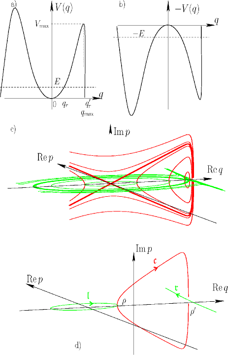
Figure 8: (colour online) The escape rate at energy $E$ from an island created by a confining potential $V$ whose shape is shown in a) can be semiclassically computed in terms of complex classical orbits where one canonical coordinate, say $q$, is kept real. In phase-space, this trajectory appears to be a concatenation of two types of curves that join on the $(\operatorname{Re}q)$-axis: 1) a trajectory that lies in the phase-space plane $(\operatorname{Re}q,\operatorname{Re}p)$ with real variations of $t$ at energy $E$ with the potential $V$ and 2) a trajectory that lies in the phase-space plane $(\operatorname{Re}q,\operatorname{Im}p)$ with imaginary variations of $t$ at energy $-E$ with the potential $-V$ shown in b). In c) a family of constant energy curves is shown (horizontal green for the first type, vertical red for the second type). In d) for a given energy, we show how three curves $\mathfrak{l},\mathfrak{c},\mathfrak{r}$ glue together at the turning points.

So far we have focused our analysis of tunnelling in bounded systems only, but the philosophy we presented here can be extended to more general situations. For instance, let us show how we can compute the escape rate from a metastable state localised in a confining potential $V$ whose shape has the form given in Fig. 8 a). The potential has a local minimum at $q=0$ (say $V_{\textrm{min}}=0$) and an energy barrier for $0<q<q_{\textrm{max}}$ whose height is $V_{\mathrm{max}}$. For $q>q_{\textrm{max}}$, the potential remains non-positive and therefore in real phase-space ($\operatorname{Re}p$, $\operatorname{Re}q$), $V$ defines around the origin an island of stability made of tori with positive energy. One state whose Husimi distribution is initially localised in the island, say a quasi-mode $\mathinner{|{\Phi_{n}}\rangle}$ at energy $0<E_{n}<V_{\mathrm{max}}$, will progressively decay outside the well. The decay rate $\Gamma_{n}$ is then defined from the overlap:

$$\mathinner{\langle{\Phi_{n}}|}\hat{U}(T)\mathinner{|{\Phi_{n}}\rangle}=\mathrm{e}^{-\Gamma_{n}T/2-{\mathrm{i}}E_{n}T/\hbar}\;.$$ (67)

If we choose a complex $T$ such that

$$|\Gamma_{n}T|\ll 1\;,$$ (68)

then we obtain a trace formula for $\Gamma_{n}$ with the help of the projector-like operator $\hat{\varPi}_{n}$

$$\Gamma_{n}\simeq-\frac{2}{\operatorname{Im}T}\operatorname{Im}\left(\mathrm{e}^{{\mathrm{i}}E_{n}T/\hbar}\operatorname*{tr}\big{(}\hat{\varPi}_{n}\hat{U}(T)\big{)}\right)$$ (69)

which allows an explicit semiclassical expansion in terms of classical solutions with a complex time path. The dominant contributions will be provided by periodic orbits in time $T$ with real $q$ starting on the torus at energy $E_{n}$, then, while ${\mathrm{i}}\mathrm{d}t/\mathrm{d}s>0$, going forth outside the well before coming back to its initial starting point (Fig. 8 c, d)). Then, up to a dimensionless factor $f_{n}$ of order one, we get

$$\Gamma_{n}\simeq\frac{f_{n}}{T_{\mathfrak{c}}(E_{n})}\mathrm{e}^{-\tilde{S}_{\mathfrak{c}}(E_{n})/\hbar}$$ (70)

with

$$\tilde{S}_{\mathfrak{c}}(E)\overset{\mathrm{def}}{=}2\int_{q_{r}(E)}^{q^{\prime}_{r}(E)}\!\!\sqrt{2\big{(}V(q)-E\big{)}}\,\mathrm{d}q$$ (71)

where $0<q_{r}(E)<q_{r}^{\prime}(E)$ are the two right turning points at energy $E$. Here we have supposed that the action between the two left turning points is larger than (71) and gives a subdominant contribution. If the potential is symmetric, two symmetric complex orbits would contribute with the same weight and therefore the escape rate should twice as large. In the case of an island with sharp boundaries around $q_{\textrm{max}}$, $\tilde{S}_{\mathfrak{c}}(E)$ which is the area enclosed by the primitive orbit $\mathfrak{c}$ (Fig. 8 d) is mainly given by the portion of $\mathfrak{c}$ where we can keep an harmonic approximation for the potential: $V(q)\sim\omega^{2}q^{2}/2$, $q_{r}(E)\simeq\sqrt{2E}/\omega$, $q^{\prime}_{r}(E)\simeq\sqrt{A/(\pi\omega)}$ where $A$ is the area of the island in the real phase space. Then, with $a\;\smash{\overset{\text{\tiny def}}{=}}\omega A/(2\pi E)$, we have

$$\tilde{S}_{\mathfrak{c}}(E)\simeq\frac{2E}{\omega}\left[\sqrt{a}\sqrt{a-1}-\ln\big{(}\sqrt{a}+\sqrt{a-1}\,\big{)}\right]\;.$$ (72)

Inserting this expression in (69) with $E_{n}\simeq(n+1/2)\hbar\omega$, we exactly recover the expression (5) used in Backer+08a with an elegant and simple interpretation. The chaotic sea that surrounds the integrable island in the mixed system considered by Bäcker et al. acts as a sharp effective potential barrier as the one draw in picture 8; our complex trajectory that allows to escape from the regular region has its main features governed by the integrable (and even harmonic) approximation of the dynamics about the island, following precisely the general philosophy of Backer+08a and Lock+09a . This computation of the “direct” tunnelling (by opposition to resonant tunnelling where the model of a pure quadratic kinetic energy fails) can also be reproduced within the standard one-dimensional JWKB theory used for computing transmission coefficients.

Here again, we can check easily that the traditionnal instanton method is included in our approach : The regime $\Re T\to 0$ selects the instanton solution and provides the escape rate from the equilibrium point as given by equation (2.47) of (Coleman85a, , chap. 7).

VIII Conclusions

The explicit semiclassical expansions of trace formulae for tunnelling splittings (or escape rates) in terms of classical orbits constructed with complex-time paths provide an interesting alternative approach to Herring formulae essentially because they do not require to analytically continue the wave functions in the complex plane. In multidimensional tunnelling and/or for a non-autonomous Hamiltonian system, the generic lack of constants of motion isolates the stable islands (if any) from each other by chaotic seas. The analytic continuation of the kam tori that build the islands is prevented by the existence of natural boundaries (see for instance the recent discussion in (Shudo+09a, , part II, appendix B) and references therein). The approach we have presented here seems to circumvent these difficulties but, of course, the problem of how to select, with an appropriate $[t]$, the relevant trajectories among an a priori exponentially growing number of classical complex solutions remains open. We expect the tunnelling splittings between two states at energy around $E$ localised in two symmetric islands to be approximated by the expansion of the form

$$\big{|}\frac{f\hbar}{T}\sum_{[\rho_{1},\rho_{2},\dots]}\mathrm{e}^{{\mathrm{i}}\sum_{i=1}^{N}w_{i}[\tilde{S}_{i}(E_{n})/\hbar-\pi]}\mathrm{e}^{-\sum_{j=1}^{M}w^{\prime}_{j}[\tilde{S}^{\prime}_{j}(E_{n})/\hbar]}\big{|}$$ (73)

where the sum runs over all possible sequences of turning points $[\rho_{1},\rho_{2},\dots]$ at energy $E$ such that we can choose a complex-time path that leads to a trajectory, made of primitive orbits, that connects in time $T$ the two (real) tori. The winding $\{w_{i}\}$ and the actions $\{S_{i}\}$ (resp. $\{w^{\prime}_{j}\}$ and $\{\tilde{S}^{\prime}_{j}\}$) refer to the primitive orbits obtained when the variations $\mathrm{d}t/\mathrm{d}s$ are purely real (resp. purely imaginary). For dimensions larger that one, the dimensionless prefactor $f$ may appear as a power law in $\hbar$. Here, inspired by the study in section VI, we can qualitatively see how the constructive interferences between repeated paths emerge in a speckle-like forest because of the presence of resonances. As shown in Mouchet07a , a progressive complex rotation of time provides a natural way to select the main resonance effects. If we want to expand the splittings (or the escape rates) according to elementary process as proposed in Lock+09a , our approach offers a promising tool to interpret and compute semiclassically all of the ingredients of such an expansion.

Appendix A

In this appendix, we derive the dominant contributions (19) to the traces involved in (9). Both cases $\operatorname*{tr}\!\big{(}\hat{U}(T)\big{)}$ and $\operatorname*{tr}\!\big{(}\hat{\mathsf{S}}\,\hat{U}(T)\big{)}$ will be treated simultaneously by defining the sign $\eta$ to be $+1$ in the first case and $-1$ in the second case. The semiclassical arguments underpinning the derivation are relatively standard and may be found in one way or another in the literature. For instance, the contribution (86) for $\eta=1$ can be found in (Dashen+74a, , eq. (2.12)) within a more restricted context (see also (Haake01a, , chap. 8)). Nevertheless we found it useful to provide all the steps in the precise context of this work, not only to render the presentation self-contained, but also because we are working in the time domain with general Hamiltonians that have not necessarily the form (1).

Given a $[t]$, for any classical phase-space path $\mathfrak{o}$, we can consider the final coordinates $(p_{f},q_{f})$ at time $t(s_{f})=T$ as smooth functions of the initial coordinates $(p_{i},q_{i})$ at time $t(s_{i})=0$. The monodromy matrix $M_{\mathfrak{o}}$ is defined as the differential of these functions: to first order, an initial small perturbation implies the final perturbation

$$\binom{\delta p_{f}}{\delta q_{f}}=\begin{pmatrix}M_{\mathfrak{o},11}&M_{\mathfrak{o},12}\\ M_{\mathfrak{o},21}&M_{\mathfrak{o},22}\end{pmatrix}\binom{\delta p_{i}}{\delta q_{i}}\;.$$ (74)

The sub-matrices can be expressed from the second derivatives of $S_{\mathfrak{o}}(q_{f},q_{i};T)$ by differentiating equations (18):

$$M_{\mathfrak{o},11} =-\partial^{2}_{q_{f}q_{f}}S_{\mathfrak{o}}\left(\partial^{2}_{q_{f}q_{i}}S_{\mathfrak{o}}\right)^{-1};$$ (75a)

$$M_{\mathfrak{o},12} =\partial^{2}_{q_{f}q_{i}}S_{\mathfrak{o}}-\partial^{2}_{q_{f}q_{f}}S_{\mathfrak{o}}\left(\partial^{2}_{q_{f}q_{i}}S_{\mathfrak{o}}\right)^{-1}\partial^{2}_{q_{i}q_{i}}S_{\mathfrak{o}}\;;$$ (75b)

$$M_{\mathfrak{o},21} =-\left(\partial^{2}_{q_{f}q_{i}}S_{\mathfrak{o}}\right)^{-1};$$ (75c)

$$M_{\mathfrak{o},22} =-\left(\partial^{2}_{q_{f}q_{i}}S_{\mathfrak{o}}\right)^{-1}\partial^{2}_{q_{i}q_{i}}S_{\mathfrak{o}}\;;$$ (75d)

provided that $\partial^{2}_{q_{f}q_{i}}S_{\mathfrak{o}}$ is invertible. Equations (75a,c,d) can be inverted in

$$\partial^{2}_{q_{f}q_{i}}S_{\mathfrak{o}} =-(M_{\mathfrak{o},21})^{-1}\;;$$ (76a)

$$\partial^{2}_{q_{i}q_{i}}S_{\mathfrak{o}} =(M_{\mathfrak{o},21})^{-1}M_{\mathfrak{o},22}\;;$$ (76b)

$$\partial^{2}_{q_{f}q_{f}}S_{\mathfrak{o}} =M_{\mathfrak{o},11}(M_{\mathfrak{o},21})^{-1}\;;$$ (76c)

while (75b) provides

$$M_{\mathfrak{o},12}=-(M_{\mathfrak{o},21})^{-1}+M_{\mathfrak{o},11}(M_{\mathfrak{o},21})^{-1}M_{\mathfrak{o},22}$$ (77)

which is nothing but the expression that $\det M_{\mathfrak{o}}=1$ once we use the identity

$$\det\begin{pmatrix}A&B\\ C&D\end{pmatrix}=\det(CAC^{-1}D-CB)$$ (78)

where $(A,B,C,D)$ are square matrices of the same size and $C$ is invertible.

Coming back to the oscillating integral (17), if the integration path can be deformed in order to pass through an isolated critical point $q_{c}$ of $q\mapsto S_{\mathfrak{o}}(\eta q,q,T)$, we will have a contribution of the form

$$\frac{\displaystyle\sqrt{\det\left(\frac{\partial^{2}S_{\mathfrak{o}}}{\partial q_{i}\partial q_{f}}\right)}}{\displaystyle\sqrt{\det\left(-\frac{\partial^{2}\big{(}S_{\mathfrak{o}}(\eta q,q;T)\big{)}}{\partial q\partial q}\right)}}\;\mathrm{e}^{{\mathrm{i}}S_{\mathfrak{o}}/\hbar}$$ (79)

where all the functions are evaluated at $(\eta q_{c},q_{c},T)$. Physically $q_{c}$ is interpreted as the initial position of the phase space paths $\mathfrak{o}$ such that $(p_{f},q_{f})=(\eta p_{i},\eta q_{i})$. With the help of (76), the prefactor of the exponential can be written as $\big{[}\det\big{(}M_{\mathfrak{o},22}+M_{\mathfrak{o},21}M_{\mathfrak{o},11}(M_{\mathfrak{o},21})^{-1}-2\eta\big{)}\big{]}^{-1/2}$ up to a global sign. Using (78) again, the contribution (79) can be written as

$$\frac{(-1)^{\nu_{\mathfrak{o}}}}{\sqrt{(-\eta)^{\textsc{d}}\det(1-\eta M_{\mathfrak{o}})}}\;\mathrm{e}^{{\mathrm{i}}S_{\mathfrak{o}}/\hbar}$$ (80)

where $(-1)^{\nu_{\mathfrak{o}}}$ fixes the sign of the square root and d demotes the number of degrees of freedom. Recall that in the definition of the path-integrals (12), a time-slice $\tau$ is always implicit. Let us keep for a moment an explicit discretization, for instance with $T$ being an integer multiple of $\tau$, $\mathfrak{o}$ referring to a discrete set of points, Hamilton’s equations (14) being discretized into a phase-space map, path integral (13) being turned into a discrete (Riemann) sum, etc. Then, the contribution of each of the points of a given $\mathfrak{o}$, such that $(p_{f},q_{f})=(\eta p_{i},\eta q_{i})$, is the same and remains given by (80); but this is correct only if, for a given $\tau$, $\hbar$ is small enough, because when performing the steepest-descent method on (17), one must be able to split the oscillating integral into separate contributions coming from two distinct points of $\mathfrak{o}$. In the continuous time limit, i.e. when the limit $\tau\to 0$ is taken before the semiclassical limit $\hbar\to 0$ (see [??]), the orbits $\mathfrak{o}$ of non-zero length appear as a one-dimensional continuum none of whose points can be considered separately anymore. The only isolated critical points $q_{c}$ are given by the position of some equilibrium points. Under the symmetric condition $(q_{i},p_{i})=(-p_{i},-q_{i})$, only the origin must be examined. Linearising the Hamiltonian flow about a non-degenerated fixed point $\mathfrak{e}=(p_{e},q_{e})$ leads to a monodromy matrix whose eigenvalues can be collected by pairs $\exp(\pm\lambda_{\mathfrak{e},\alpha}T)$ where $\{\lambda_{\mathfrak{e},\alpha}\}_{\alpha=1,\dots\textsc{d}}$ are the Lyapunov exponents. Then (80) becomes

$$\frac{(-1)^{\nu_{\mathfrak{e}}}\,\mathrm{e}^{-{\mathrm{i}}H(p_{e},q_{e})T/\hbar}}{\prod_{\alpha=1}^{\textsc{d}}(\mathrm{e}^{\lambda_{\mathfrak{e},\alpha}T/2}-\eta\mathrm{e}^{-\lambda_{\mathfrak{e},\alpha}T/2})}$$ (81)

with a possible adjustment of the sign. For a generic choice of $T$, the denominator does not vanish.

For a non-zero length path $\mathfrak{o}$, the critical $q$’s are degenerate along the trajectory; for a system with several degrees of freedom, one must treat separately the (gaussian) integrals on the transverse coordinates $q_{\perp}$ along which $S_{\mathfrak{o}}(\eta q,q,T)$ varies (quadratically) from the longitudinal coordinates $q_{\parallel}$ along which $S_{\mathfrak{o}}(\eta q,q,T)$ is constant. Of course, the dimensions of $q_{\perp}$ and $q_{\parallel}$ depend crucially on the presence of kam tori. However, multidimensional tunnelling is beyond the scope of this paper and, the quantitative studies presented here concern one-dimensional systems only. The contribution to the trace of such a path is then, up to a global sign,

$$\frac{\mathrm{e}^{{\mathrm{i}}S_{\mathfrak{o}}/\hbar}\;}{\sqrt{-2{\mathrm{i}}\pi\hbar}}\int\mathrm{d}q\sqrt{\frac{\partial^{2}S_{\mathfrak{o}}}{\partial q_{i}\partial q_{f}}\bigg{|}}_{(\eta q,q;T)}.$$ (82)

The conservation of energy along $\mathfrak{o}$, $H(p,q)=E$, implicitly defines a function $p(q,E)$ in the neighbourhood of any point where $\partial_{p}H\neq 0$. Globally along the trajectory $\mathfrak{o}$, we may encounter several possible branches $p_{\beta}(q,E)$ for the graph of these functions (the two possible signs of a square root when the Hamiltonian has the form (1)) which become singular but pairwise connect smoothly at the turning points, defined by $\partial_{p}H=0$. A relation between $E$, $T$, $q_{f}$ and $q_{i}$ can be obtained by integrating $\int_{s_{i}}^{s_{f}}(\mathrm{d}t/\mathrm{d}s)\,\mathrm{d}s$ and using (14b):

$$T=T_{\mathfrak{o}}(q_{f},q_{i};E)\overset{\mathrm{def}}{=}\int_{s_{i}}^{s_{f}}\frac{\mathrm{d}q/\mathrm{d}s}{\partial_{p}H\Big{(}p\big{(}q(s),E\big{)},q(s)\Big{)}}\;\mathrm{d}s\;.$$ (83)

Everywhere but at the turning points, the value of $s$ dictates the choice of the branch used for the integrand. This relation implicitly defines $E_{\mathfrak{o}}(q_{f},q_{i};T)$. The usual expression for the derivative of implicit functions leads to the relations: $\partial_{\!E}\,p\mathop{=}1/\partial_{p}H$ and $\partial_{q_{i}}E_{\mathfrak{o}}\mathop{=}-\partial_{q_{i}}T_{\mathfrak{o}}/\partial_{E}T_{\mathfrak{o}}\mathop{=}\partial_{T}E_{\mathfrak{o}}/\partial_{p}H(p_{i},q_{i})$. If we differentiate (18b) with respect to $q_{i}$ when $p_{f}$ is given by $p\big{(}q_{f},E_{\mathfrak{o}}(q_{f},q_{i},T)\big{)}$, we obtain

$$\frac{\partial^{2}S_{\mathfrak{o}}}{\partial q_{i}\partial q_{f}}\bigg{|}_{(q_{f},q_{i};T)}=\frac{1}{\partial_{p}H(p_{f},q_{f})}\frac{1}{\partial_{p}H(p_{i},q_{i})}\frac{\partial E_{\mathfrak{o}}}{\partial T}\bigg{|}_{(q_{f},q_{i};T)}\;.$$ (84)

With property (3), we get $\partial_{p}H(\eta p,\eta q)=\eta\partial_{p}H(p,q)$ and then, by differentiating (83), we have $\partial_{q}\big{(}T_{\mathfrak{o}}(\eta q,q,E)\big{)}=0$. Therefore, the energy $E_{\mathfrak{o}}$ of the path $\mathfrak{o}$ depends only on $T$, not on its starting point $q$. The square root of $\partial_{T}E_{\mathfrak{o}}(\eta q,q,T)=\mathrm{d}E_{\mathfrak{o}}/\mathrm{d}T$ can be got out from the integral in (82). When adding the contribution of each path whose starting point lie on the branch $\beta$, we obtain

$$T_{\beta}(E)\overset{\mathrm{def}}{=}\int\frac{\mathrm{d}q}{\partial_{p}H\Big{(}p_{\beta}\big{(}q,E\big{)},q\Big{)}}\;.$$ (85)

This is not exactly the right hand side of (83) because the domain of integration in (85) is the domain of the branch where the starting point of $\mathfrak{o}$ lives. Each branch $\beta$ is delimited by two turning points and $T_{\beta}$ is the time spent to go from one point to the other.

The integral (82) involves all the possible starting points for a trajectory $\mathfrak{o}$ and therefore we must add all the branches that patchwork smoothly in phase-space to form the geometrical set of points crossed by $\mathfrak{o}$. Referring to the purely geometrical quantities (i.e. independent of the choice of the parametrization), we have the contribution

$$(-1)^{\mu_{\mathfrak{o}}}\frac{\left(\sum_{\beta}T_{\beta}\right)}{\sqrt{-2\eta{\mathrm{i}}\pi\hbar}}\sqrt{\frac{\mathrm{d}E_{\mathfrak{o}}}{\mathrm{d}T}}\;\mathrm{e}^{{\mathrm{i}}S_{\mathfrak{o}}/\hbar}$$ (86)

only if $T_{\mathfrak{o}}=T$; for $\eta=+1$ the path $\mathfrak{o}$ is a periodic orbit and, for $\eta=-1$, the path $\mathfrak{o}$ is half a symmetric periodic orbit (the whole periodic orbit being of period equal to $2T$). The sum concerns all the geometrical branches $\beta$ crossed by $\mathfrak{o}$ (even if $\mathfrak{o}$ passes several times by the same points, each branch is only counted once). As before, the conversion of a product of two square roots of complex numbers to the square root of the product may introduce a sign that can be absorbed in the definition of $\mu_{\mathfrak{o}}$; the exact computation of the index $\mu_{\mathfrak{o}}$ is difficult but since it may change at the bifurcation points only, where the semiclassical approximation fails, it is sufficient to know that it depends on the nature and the number of the turning points encountered on $\mathfrak{o}$. Therefore it is an additive quantity when several primitive orbits are repeated or concatenated together.

Appendix B

In this appendix we explain how to obtain the asymptotic expansions (33) as $E\to 0^{+}$.

First consider $\tilde{S}_{\mathfrak{r}}$ and split it in two parts $\tilde{S}_{+}+\tilde{S}_{-}$ where

$$\tilde{S}_{+} \overset{\mathrm{def}}{=} \int_{a}^{q_{r}^{\prime}(E)}\!\!2\sqrt{2\big{(}E-V(q)\big{)}}\,\mathrm{d}q\;;$$ (87a)

$$\tilde{S}_{-} \overset{\mathrm{def}}{=} \int_{q_{r}(E)}^{a}\!\!2\sqrt{2\big{(}E-V(q)\big{)}}\,\mathrm{d}q\;.$$ (87b)

Setting $\epsilon\overset{\mathrm{def}}{=}a-q_{r}(E)$, rewrite $\tilde{S}_{-}$ as

$$\tilde{S}_{-}=2\sqrt{2}\epsilon\int_{0}^{1}\sqrt{V(a-\epsilon)-V(a-s\epsilon)}\,\mathrm{d}s,$$ (88)

Now expand the integrand as a power series in $\epsilon$ up to the fourth order, compute the integrals that appear in each coefficient and insert the expansion of $\epsilon$ in $E$ obtained from the implicit equation $V(a-\epsilon)=E$:

$$\epsilon=\frac{\sqrt{2}}{\omega}\,\sqrt{E}+\frac{V^{(3)}(a)}{3\omega^{4}}\,E\\ -\frac{\sqrt{2}\Big{(}3\omega^{2}V^{(4)}(a)-5\big{(}V^{(3)}(a)\big{)}^{2}\Big{)}}{36\omega^{7}}\,E^{3/2}+\mathrm{O}(E^{2})\;.$$ (89)

Proceed in an analogous way for the computation of the first three terms of the asymptotic expansion in $\sqrt{E}$ for $\tilde{S}_{+}$. When summing $S_{+}$ and $S_{-}$, expression (33b) is obtained with (35).

The expansion of $\tilde{S}_{\mathfrak{c}}$ is more subtle since it is not differentiable at $E=0$. Its derivative is given by

$$\frac{\mathrm{d}\tilde{S}_{\mathfrak{c}}}{\mathrm{d}E}=-\int_{\epsilon}^{a}L(s,\epsilon)\,\mathrm{d}s$$ (90)

where we denote $\epsilon\overset{\mathrm{def}}{=}a-q_{r}(E)$ and define

$$L(s,\epsilon)\overset{\mathrm{def}}{=}\frac{2\sqrt{2}}{\sqrt{V(a-s)-V(a-\epsilon})}\;.$$ (91)

The function $L(s,\epsilon)$ is not continuous but we can extract the discontinuous part from

$$L(s,\epsilon)=\frac{4}{\omega\sqrt{s^{2}-\epsilon^{2}}}\left(\!\!1+\!\!\sum_{n\geqslant 3}\frac{(-1)^{n}2V^{(n)}(a)}{n!}\frac{s^{n}-\epsilon^{n}}{s^{2}-\epsilon^{2}}\!\right)^{\!\!\!\!-\frac{1}{2}}$$ (92)

by expanding the last factor:

$$L(s,\epsilon)=\frac{4}{\omega\sqrt{s^{2}-\epsilon^{2}}}+\frac{2V^{(3)}(a)}{3\omega^{3}}\frac{s^{3}-\epsilon^{3}}{(s^{2}-\epsilon^{2})^{3/2}}+M(s,\epsilon)$$ (93)

where now $M(s,\epsilon)$ is a continuous function of its two variables. Then, a standard theorem in analysis assures that $\epsilon\mapsto\int_{\epsilon}^{a}M(s,\epsilon)\,\mathrm{d}s$ is continuous and its limit when $\epsilon\to 0$ is

$$\int_{0}^{a}M(s,0)\,\mathrm{d}s = \int_{0}^{a}\left(L(s,0)-\frac{4}{\omega s}-\frac{2V^{(3)}(a)}{3\omega^{3}}\right)\mathrm{d}s$$ (94)

$$= \frac{4A}{\omega}-\frac{2aV^{(3)}(a)}{3\omega^{3}}$$

with $A$ given by (34). The two other integrals obtained by inserting (93) in the right hand side of (90) can be computed exactly and expanded as $\epsilon\to 0^{+}$ up to order $\mathrm{o}(1)$. Then, inserting (89), we obtain

$$\frac{\mathrm{d}\tilde{S}_{\mathfrak{c}}}{\mathrm{d}E}=\frac{4}{\omega}\ln\left(\frac{\sqrt{2E}}{2a\omega}\right)-\frac{4A}{\omega}+\mathrm{o}(1)\;.$$ (95)

Its integration leads directly to (33a).

Appendix C

The quasi-mode $\mathinner{|{\Phi_{n}}\rangle}\;\smash{\overset{\text{\tiny def}}{=}}(\mathinner{|{\phi_{n}^{+}}\rangle}+\mathinner{|{\phi_{n}^{-}}\rangle})/\sqrt{2}$ is localised on one torus at energy $E^{+}_{n}\simeq E^{-}_{n}$. Standard jwkb techniques Keller58a ; Percival77a provide a semiclassical approximation to its wave function:

$$\Phi^{\mathrm{s.c.}}_{n}(q)=\frac{1}{\sqrt{\sum_{\beta}T_{\beta}(E_{n})}}\sum_{\beta}\frac{A_{n,\beta}}{\sqrt{\partial_{p}H\big{(}p_{\beta}(q,E_{n}),q\big{)}}}\\ \times\exp{\left({\mathrm{i}}\int^{q}_{b_{\beta}}p_{\beta}(x,E_{n})\,\mathrm{d}x/\hbar\right)}$$ (96)

($\beta$ labels the possible several branches of the torus, $A_{n,\beta}$ are dimensionless coefficients of unit modulus, ${b_{\beta}}$ is a base point of the branch $\beta$ and $T_{\beta}(E_{n})$ the characteristic time (85) spent on the branch $\beta$). Within the semiclassical approximation, it is, therefore, consistent to construct $\varPi_{n}(q^{\prime},q)$ by substituting (96) in the matrix elements of the projector operator $\mathinner{|{\phi_{n}^{+}}\rangle}\mathinner{\langle{\phi_{n}^{+}}|}+\mathinner{|{\phi_{n}^{-}}\rangle}\mathinner{\langle{\phi_{n}^{-}}|}=\mathinner{|{\Phi_{n}}\rangle}\mathinner{\langle{\Phi_{n}}|}+\hat{\mathsf{S}}\mathinner{|{\Phi_{n}}\rangle}\mathinner{\langle{\Phi_{n}}|}\hat{\mathsf{S}}$. From the integral (20)

$$2\int\mathrm{d}q\,\mathrm{d}q^{\prime}\;\Phi_{n}^{\mathrm{s.c.}}(q)\,\big{(}\Phi_{n}^{\mathrm{s.c.}}(q^{\prime})\big{)}^{*}\,G(\eta q^{\prime},q;T)\;,$$ (97)

when we insert the semiclassical expressions (16), we obtain a sum of integrals of the form

$$\int\mathrm{d}q\,\mathrm{d}q^{\prime}\frac{\text{\Large e}^{\displaystyle\frac{{\mathrm{i}}}{\hbar}\int^{q}_{b_{\beta}}p_{\beta}(x,E_{n})\,\mathrm{d}x}}{\sqrt{\partial_{p}H\big{(}p_{\beta}(q,E_{n}),q\big{)}}}\frac{\text{\Large e}^{\displaystyle-\frac{{\mathrm{i}}}{\hbar}\int^{q^{\prime}}_{b_{\beta^{\prime}}}p_{\beta^{\prime}}(x,E_{n})\,\mathrm{d}x}}{\sqrt{\partial_{p}H\big{(}p_{\beta^{\prime}}(\eta q^{\prime},E_{n}),q^{\prime}\big{)}}}\times\\ \sqrt{\frac{\partial^{2}S_{\mathfrak{o}}}{\partial q_{i}\partial q_{f}}\bigg{|}}_{(\eta q^{\prime},q;T)}\mathrm{e}^{{\mathrm{i}}S_{\mathfrak{o}}(\eta q^{\prime},q;T)/\hbar}\;.$$ (98)

The stationary conditions

$$p_{\beta}(q,E_{n}) =- \partial_{q_{i}}S_{\mathfrak{o}}(\eta q^{\prime},q;T)\;;$$ (99a)

$$\eta p_{\beta^{\prime}}(q^{\prime},E_{n}) = \partial_{q_{f}}S_{\mathfrak{o}}(\eta q^{\prime},q;T)$$ (99b)

select the classical trajectories $\mathfrak{o}$ with energy $E_{n}$ that go from $(p_{i},q_{i})=(p_{\beta}(q,E_{n}),q)$ at $t(s_{i})=0$ to  $(p_{f},q_{f})=(\eta p_{\beta^{\prime}}(q^{\prime},E_{n}),\eta q^{\prime})$ at time $t(s_{f})=T$. Then the value of the exponent

$$S_{\mathfrak{o},\beta,\beta^{\prime}}(E_{n},T)=-E_{n}T+\tilde{S}_{\mathfrak{o}}(b_{\beta^{\prime}},b_{\beta},E_{n})$$ (100)

depends only on the branches where the starting and ending points lie and not on the precise location of these points on the branches. Since $q$ and $q^{\prime}$ correspond to the same torus, such a trajectory must connect the two symmetric tori for $\eta=-1$. At a given $E_{n}$ and $T$, for a fixed $q=q_{i}$ on the branch $\beta$, $q_{f}$ and $\beta^{\prime}$ are uniquely given and we can make the stationary phase approximation for the integral on $q^{\prime}$. Then if we insert (83) at energy $E_{n}$ into (99) and differentiate it with respect to $q$ or $q^{\prime}$, we obtain some identities that, with (84), allow us to simplify the combination of the prefactors and the remaining integral in $q$ turns out to be precisely of the form of the right hand side of (85). A priori, the domain of integration is included in the domain of the branch $\beta$ but is not necessarily equal to it because when sliding the starting point on the whole branch $\beta$, the endpoint may cross a turning point and correspond to a jump of $\beta^{\prime}$. However, we obtain characteristic times that depend only on the geometry of the orbit, not on the number of times the considered branch may be repeated as $s$ goes from $s_{i}$ to $s_{f}$. As discussed in the case of the double well, if there exist different topological classes of $\mathfrak{o}$, each of them being characterised by an ordered sequence of turning points $[\rho_{1},\rho_{2},\dots]$, we must add such contributions. Then, using directly $\operatorname*{tr}\!\big{(}\hat{\varPi}_{n}\hat{U}(T)\big{)}\simeq 2\mathrm{e}^{-{\mathrm{i}}E_{n}T/\hbar}$, we have proven that

$$\Delta_{n}(T)\underset{\hbar\to 0}{\sim}\frac{\hbar}{T}\!\!\!\sum_{[\rho_{1},\rho_{2},\dots]}\!\!\!(-1)^{\mu_{\mathfrak{o}}}A_{\beta,\beta^{\prime}}(E_{n},T)\,\mathrm{e}^{{\mathrm{i}}\tilde{S}_{\mathfrak{o}}(b_{\beta^{\prime}},b_{\beta},E_{n})/\hbar}$$ (101)

where the sum runs over all the sequences of turning points on the section $\mathfrak{s}$ at energy $E_{n}$ where one canonical variable is maintained real. There must exist for such a sequence, one half symmetric orbit $\mathfrak{o}$ starting on the branch $\beta$ of the torus at energy $E_{n}$, crossing successively all the sequences $[\rho_{1},\rho_{2},\dots]$ and ending on the branch $\beta^{\prime}$ at time $T$. The dimensionless coefficients $A_{\beta,\beta^{\prime}}(E_{n},T)$ have a $\hbar$-independent modulus of order one and depend only on the geometrical properties of the branches. If some parts of the trajectory are repeated, their repetition numbers do not appear in $A_{\beta,\beta^{\prime}}(E_{n},T)$ but only in the cumulative quantities: the index $\mu_{\mathfrak{o}}$ and the action $\tilde{S}_{\mathfrak{o}}(b_{\beta^{\prime}},b_{\beta},E_{n})$ given by

$$\tilde{S}_{\mathfrak{o}}(b_{\beta^{\prime}},b_{\beta},E_{n})=\int^{s_{f}}_{s_{i}}p(s)\frac{\mathrm{d}q}{\mathrm{d}s}\,\mathrm{d}s\\ +\int_{b_{\beta}}^{q(s_{i})}p_{\beta}(x,E_{n})\,\mathrm{d}x-\int_{b_{\beta^{\prime}}}^{q(s_{f})}p_{\beta^{\prime}}(x,E_{n})\,\mathrm{d}x\;.$$ (102)

In the case of two branches, the computation of the coefficient can be done exactly using the appropriate choice of phase conventions for the base points $b_{\beta}$ and $A_{n,\beta}$; we obtain:

$$A_{\beta,\beta^{\prime}}(E_{n},T)=-1/2\;.$$ (103)

We illustrate in the main body of this article, how to compute the sum in the right hand side of (101).

References

- (1) Instantons in gauge theories, Vol. 5 of Advanced Series in Mathematical Physics, edited by M. A. Shifman (World Scientific, Singapore, 1994).
- (2) S. Coleman, Aspects of symmetry (selected Erice lectures) (Cambridge University Press, Cambridge, 1985).
- (3) J. Zinn-Justin, Quantum Field Theory and Critical Phenomena (4th ed.), Vol. 113 of International Series of Monographs on Physics (Clarendon Press Oxford, Oxford, 2002).
- (4) M. J. Davis and E. J. Heller, J. Chem. Phys. 75, 246 (1981).
- (5) N. T. Maitra and E. J. Heller, Phys. Rev. A 54, 4763 (1996).
- (6) N. T. Maitra and E. J. Heller, Phys. Rev. Lett. 78, 3035 (1997).
- (7) K. F. Freed, J. Chem. Phys. 56, 692 (1972).
- (8) T. F. George and W. H. Miller, J. Chem. Phys. 56, 5522 (1972).
- (9) W. H. Miller, Adv. Chem. Phys. 25, 69 (1974).
- (10) U. Weiss and W. Haeffner, Phys. Rev. D 27, 2916 (1983).
- (11) R. D. Carlitz and D. A. Nicole, Ann. Physics 164, 411 (1985).
- (12) E. M. Ilgenfritz and H. Perlt, J. Phys. A 25, 5729 (1992).
- (13) N. T. Maitra and E. J. Heller, in Classical, semiclassical and quantum dynamics in atoms, edited by H. Friedrich and B. Eckhardt (Springer-Verlag, Berlin, 1997), pp. 94–111.
- (14) S. C. Creagh and N. D. Whelan, Ann. Physics 272, 196 (1999).
- (15) A. M. Ozorio de Almeida, J. Phys. Chem. 88, 6139 (1984).
- (16) D. Farrelly and T. Uzer, J. Chem. Phys. 85, 308 (1986).
- (17) E. J. Heller, J. Phys. Chem. 99,, 2625 (1995).
- (18) S. Tomsovic, J. Phys. A 31, 9469 (1998).
- (19) D. W. Mclaughlin, J. Math. Phys. 13, 1099 (1972).
- (20) Y. Zohta, Phys. Rev. D 41, 7879 (1990).
- (21) D. Bohm, Quantum theory (Prentice Hall, Englewood Cliffs, N. J., 1951).
- (22) K. Takahashi and N. Saitô, Phys. Rev. Lett. 55, 645 (1985).
- (23) E. J. Heller, in Chaos et Physique Quantique—Chaos and Quantum Physics, Les Houches, école d’été de physique théorique 1989, session LII, edited by M. Giannoni, A. Voros, and J. Zinn-Justin (North-Holland, Amsterdam, 1991), pp. 547–663.
- (24) G. Torres-Vega and J. H. Frederick, J. Chem. Phys. 93, 8862 (1990).
- (25) M. Wilkinson, Physica D 21, 341 (1986).
- (26) S. C. Creagh, in Tunneling in complex systems, Vol. 5 of Proceedings from the Institute for Nuclear Theory, edited by S. Tomsovic (World Scientific Publishing, Singapore, 1997), pp. 35–100.
- (27) A. Garg, Amer. J. Phys. 68, 430 (2000).
- (28) A. Mouchet, J. Phys. A 40, F663 (2007).
- (29) A. Shudo and K. S. Ikeda, Phys. Rev. Lett. 76, 4151 (1996).
- (30) A. Shudo, Y. Ishii, and K. S. Ikeda, J. Phys. A 42, 265101 & 265102 (2009).
- (31) J. M. Robbins, S. C. Creagh, and R. G. Littlejohn, Phys. Rev. A 39, 2838 (1990).
- (32) H. J. Korsch and Glück, Eur. J. Phys. 23, 413 (2002).
- (33) L. D. Landau and E. M. Lifshitz, Quantum Mechanics (non relativistic theory), Vol. 3 of Course of Theoretical Physics (Pergamon Press, Oxford, 1977), 3rd edition.
- (34) E. Gildener and A. Patrascioiu, Phys. Rev. D 16, 423 (1977).
- (35) T. Connor, J. N. L.and Uzer, R. A. Marcus, and A. D. Smith, J. Chem. Phys. 80, 5095 (1984).
- (36) M. Abramowitz and I. A. Segun, Handbook of mathematical functions (Dover publications, New York, 1965).
- (37) I. S. Gradshteyn and I. M. Ryzhik, Table of Integrals, Series, and Products (Academic Press, New York and London, 1965).
- (38) D. Khuat-duy and P. Lebœuf, Appl. Phys. Lett. 63, 1903 (1993).
- (39) A. Bäcker, R. Ketzmerick, S. Löck, and L. Schilling, Phys. Rev. Lett. 100, 104101 (2008).
- (40) S. Löck, A. Bäcker, R. Ketzmerick, and P. Schlagheck, Phys. Rev. Lett. 104, 104101 (2010).
- (41) R. F. Dashen, B. Hasslacher, and A. Neveu, Phys. Rev. D 10, 4114 (1974).
- (42) F. Haake, Quantum Signatures of Chaos (Springer-Verlag, Berlin, 2001).
- (43) J. B. Keller, Ann. Physics 4, 180 (1958).
- (44) I. C. Percival, Adv. Chem. Phys. 36, 1 (1977).
- (45) S. C. Creagh and N. D. Whelan, Phys. Rev. Lett. 77, 4975 (1996).
- (46) S. Tomsovic and D. Ullmo, Phys. Rev. E 50, 145 (1994).
- (47) F. Leyvraz and D. Ullmo, J. Phys. A 29, 2529 (1996).