Revisiting Marginal Regression

Abstract

The lasso has become an important practical tool for high dimensional regression as well as the object of intense theoretical investigation. But despite the availability of efficient algorithms, the lasso remains computationally demanding in regression problems where the number of variables vastly exceeds the number of data points. A much older method, marginal regression, largely displaced by the lasso, offers a promising alternative in this case. Computation for marginal regression is practical even when the dimension is very high. In this paper, we study the relative performance of the lasso and marginal regression for regression problems in three different regimes: (a) exact reconstruction in the noise-free and noisy cases when design and coefficients are fixed, (b) exact reconstruction in the noise-free case when the design is fixed but the coefficients are random, and (c) reconstruction in the noisy case where performance is measured by the number of coefficients whose sign is incorrect.

In the first regime, we compare the conditions for exact reconstruction of the two procedures, find examples where each procedure succeeds while the other fails, and characterize the advantages and disadvantages of each. In the second regime, we derive conditions under which marginal regression will provide exact reconstruction with high probability. And in the third regime, we derive rates of convergence for the procedures and offer a new partitioning of the “phase diagram,” that shows when exact or Hamming reconstruction is effective.

In addition to theoretical investigation, we present simulations showing that in practice, marginal regression and the lasso can have comparable performance, while the computational advantages of marginal regression make it feasible for much larger problems.

and

1 Introduction

A central theme in recent work on regression is that sparsity plays a critical role in effective high-dimensional inference. Consider a regression model,

$$Y=X\beta+z,$$ (1)

with response $Y=(Y_{1},\ldots,Y_{n})^{T}$, $n\times p$ design matrix $X$, coefficients $\beta=(\beta_{1},\ldots,\beta_{p})^{T}$, and noise variables $z=(z_{1},\ldots,z_{n})^{T}$. Loosely speaking, this model is high-dimensional when $p\gg n$ and is sparse when many components of $\beta$ equal zero.

An important problem in this context is variable selection: determining which components of $\beta$ are non-zero. For general $\beta$, the problem is underdetermined, but recent results have demonstrated that under particular conditions on $X$, to be discussed below, sufficient sparsity of $\beta$ allows (i) exact reconstruction of $\beta$ in the noise-free case [28] and (ii) consistent selection of the non-zero coefficients in the noisy-case [5, 3, 4, 6, 8, 16, 17, 19, 21, 28, 30, 32, 33]. Many of these results are based on showing that under sparsity constraints, a convex optimization problem that controls the $\ell^{1}$ norm of the coefficients has the same solution as an (intractable) combinatorial optimization problem that controls the number of non-zero coefficients.

In practice, the lasso [26, 5] has become one of the main tools for sparse high-dimensional variable selection, due both to its computational simplicity and its direct connection to these theoretical results. The lasso estimator in the regression problem is defined by

$$\widehat{\beta}_{\scriptscriptstyle\text{lasso}}=\mathop{\rm argmin}_{\beta}\left\|Y-X\beta\right\|_{2}^{2}+\lambda\|\beta\|_{1},$$ (2)

where $\|\beta\|_{1}=\sum_{j}|\beta_{j}|$ and $\lambda\geq 0$ is a regularization parameter that must be specified. The lasso gives rise to a convex optimization problem and thus is computationally tractable even for moderately large problems. Indeed, the LARS algorithm [14] can compute the entire solution path as a function of $\lambda$ in $O(p^{3}+np^{2})$ operations. Gradient descent algorithms for the lasso are faster in practice, but have the same computational complexity. For very large $p$, the lasso remains computationally demanding.

A much older and computationally simpler method for variable selection is marginal regression (also called correlation learning, simple thresholding [6], and sure screening [16]), in which the outcome variable is regressed on each covariate separately. To compute the marginal regression estimates for variable selection, we begin by computing the marginal regression coefficients which, assuming $X$ has been standardized, are

$$\widehat{\alpha}\equiv X^{T}Y.$$ (3)

Then, we threshold $\widehat{\alpha}$ using the tuning parameter $t>0$:

$$\widehat{\beta}_{j}=\widehat{\alpha}_{j}1\{|\widehat{\alpha}_{j}|\geq t\}.$$ (4)

This requires $O(np)$ operations, two orders faster than the lasso for $p\gg n$, and so is tractable for much larger problems.

The lasso has mostly displaced marginal regression in practice. But the computational advantage for large problems prompts a second look. Tibshirani and Witten Tibshirani-Witten:2009 [27] have found that marginal regression sometimes outperforms the lasso in predictive error. Here we revisit marginal regression as a tool for variable selection and ask whether there is any strong reason to prefer the lasso. If marginal regression exhibits comparable performance, theoretically and empirically, then it offers a plausible alternative to the lasso. Put another way: because of its simplicity, marginal regression only needs to tie to win.

In this paper, we study the relative performance of the lasso and marginal regression in three different regimes. In Section 2, we compare the conditions that guarantee exact variable selection in the noise-free case and briefly compare the conditions for consistent variable selection (i.e. sparsistency) in the noisy case. The two sets of conditions are generally overlapping, and we give examples where each procedure fails while the other succeeds. One advantage of the lasso is that, given a fixed matrix $X$, the conditions for its success hold over a larger class of $\beta$’s than that of marginal regression. On the other hand, marginal regression has a larger tolerance for collinearity than does the lasso and is somewhat easier to tune, as we illustrate in Section 2.4.

In Section 3, we consider the regime where the design matrix $X$ is fixed but the coefficient vector $\beta$ is randomly generated. We find conditions such that marginal regression performs well with overwhelming probability. The main condition, which we call faithfulness, is closely related to both the Faithfulness Condition of [21] and the Incoherence Condition of [8]. The Incoherence Condition depends only on $X$ and is thus checkable in practice, but it aims to control the worst case so is quite conservative. The Faithfulness Condition of [21] is relatively less stringent but depends on the unknown support of the parameter vector. Our version of the Faithfulness Condition strikes a compromise between the two.

Although exact variable selection has been the focus of many studies in the literature, it is rare in practice to select exactly the right variables, so it is natural to measure performance in terms of the deviation from exact selection. In Section 4, we study the convergence rates of the two procedures in Hamming distance between $\mathop{\rm sgn}({\beta})$ and $\mathop{\rm sgn}({\widehat{\beta}})$. Our main result in this section is a new partition of the parameter space into three regions I–III. In the interior of region I, exact variable selection is possible (asymptotically), and both procedures achieve this given properly chosen tuning parameters. In region II, it is possible to have a variable selection procedure that recovers most relevant variables, but not all of them. And in Region III, successful variable selection is impossible, and the optimal Hamming distance is asymptotically equivalent to the total number of relevant variables.

Finally, in Section 5 we present simulation studies showing that marginal regression and the lasso perform comparably over a range of parameters. Section 6 gives the proofs of all theorems and lemmas in the order they appear.

Notation. For a real number $x$, let $\mathop{\rm sgn}(x)$ be -1, 0, or 1 when $x<0$, $x=0$, and $x>0$; and for a vector $u\in{\mathbb{\mathchar 82\relax}}^{k}$, define $\mathop{\rm sgn}(u)=(\mathop{\rm sgn}(u_{1}),\ldots,\mathop{\rm sgn}(u_{k}))^{T}$. We will use $\|\cdot\|$, with various subscripts, to denote vector and matrix norms, and $|\cdot|$ to represent absolute value, applied component-wise when applied to vectors. With some abuse of notation, we will write $\min u$ ($\min|u|$) to denote the minimum (absolute) component of a vector $u$. Inequalities between vectors are to be understood component-wise as well.

2 Noise-Free Conditions for Exact Variable Selection

Consider a sequence of regression problems with deterministic design matrices, indexed by sample size $n$,

$$Y^{(n)}=X^{(n)}\beta^{(n)}+z^{(n)}.$$ (5)

Here, $Y^{(n)}$ and $z^{(n)}$ are $n\times 1$ response and noise vectors, respectively, $X^{(n)}$ is an $n\times p^{(n)}$ matrix and $\beta^{(n)}$ is a $p^{(n)}\times 1$ vector, where we typically assume $p^{(n)}\gg n$. We assume that $\beta^{(n)}$ is sparse in the sense that it has $s^{(n)}$ nonzero components where $s^{(n)}\ll p^{(n)}$. By rearranging $\beta^{(n)}$ without loss of generality, we can partition each $X^{(n)}$ and $\beta^{(n)}$ into “signal” and “noise” pieces, corresponding to the non-zero or zero coefficients, as follows:

$$X^{(n)}=\left(X^{(n)}_{S},X^{(n)}_{N}\right)\qquad\beta^{(n)}=\left(\begin{array}[]{c}\beta_{S}\\ \beta_{N}\end{array}\right).$$ (6)

In fact, we assume that $\beta^{(n)}_{S}\in\mathcal{M}^{s^{(n)}}_{\rho^{(n)}}$ for a sequence $\rho^{(n)}>0$ (and not converging to zero too quickly) with

$$\mathcal{M}^{k}_{a}=\left\{x=(x_{1},\ldots,x_{k})^{T}\in{\mathbb{\mathchar 82\relax}}^{k}:\;\mbox{$|x_{j}|\geq a$ for all $1\leq j\leq k$}\right\},$$ (7)

for positive integer $k$ and $a>0$. This commonly used condition on $\beta^{(n)}$ ensures that the non-zero components are not too close to zero to be indistinguishable. Finally, define the Gram matrix $C^{(n)}=({X^{(n)}})^{T}X^{(n)}$ and partition this as

$$C^{(n)}=\left(\begin{array}[]{cc}C^{(n)}_{SS}&C^{(n)}_{SN}\\ \vskip 3.0pt plus 1.0pt minus 1.0pt\cr C^{(n)}_{NS}&C^{(n)}_{NN}\end{array}\right),$$ (8)

where of course $C^{(n)}_{NS}=(C^{(n)}_{SN})^{T}$. Except in Sections 4–5, we suppose $X^{(n)}$ is normalized so that all diagonal coordinates of $C^{(n)}$ are $1$.

These ⁽ⁿ⁾ superscripts become tedious, so for the remainder of the paper, we suppress them unless necessary to show variation in $n$. The quantities $X$, $C$, $p$, $s$, $\rho$, as well as the tuning parameters $\lambda$ (for the lasso; see (2)) and $t$ (for marginal regression; see (4)) are all thus implicitly dependent on $n$. We use $\mathcal{M}_{\rho}$ to denote the space $\mathcal{M}^{s^{(n)}}_{\rho^{(n)}}$.

We will begin by specifying conditions on $C$, $\rho$, $\lambda$, and $t$ such that in the noise-free case, exact reconstruction of $\beta$ is possible for the lasso or marginal regression, for all $\beta_{S}\in\mathcal{M}_{\rho}$. These in turn lead to conditions on $C^{(n)}$, $p^{(n)}$, $s^{(n)}$, $\rho^{(n)}$, $\lambda^{(n)}$, and $t^{(n)}$ such that in the case of homoscedastic Gaussian noise, the non-zero coefficients can be selected consistently, meaning that for all sequences $\beta^{(n)}_{S}\in\mathcal{M}^{s^{(n)}}_{\rho^{(n)}}\equiv\mathcal{M}_{\rho}$,

$$P\biggl{(}\left|\mathop{\rm sgn}(\widehat{\beta}^{(n)})\right|=\left|\mathop{\rm sgn}(\beta^{(n)})\right|\biggr{)}\to 1,$$ (9)

as $n\to\infty$. (This property was dubbed sparsistency by Pradeep Ravikumar [23].) Our goal is to compare these conditions. In this section, we focus on the noise-free case, and keep the discussion on the noise case brief.

2.1 Exact reconstruction conditions for the lasso in the noise-free case

We begin by considering three conditions in the noise-free case that are now standard in the literature on the lasso:

• Condition E. The minimum eigenvalue of $C_{SS}$ is positive.

• Condition I. (Irrepresentableness)

  $$\max\left|C_{NS}C_{SS}^{-1}\,\mathop{\rm sgn}(\beta_{S})\right|\leq 1.$$

• Condition J.

  $$\min\left|\beta_{S}\,-\,\lambda C_{SS}^{-1}\,\mathop{\rm sgn}(\beta_{S})\right|>0.$$

Because $C_{SS}$ is symmetric and non-negative definite, Condition E is equivalent to $C_{SS}$ being invertible. Later we will strengthen this condition. A critical feature of Condition I is that it only depends on the sign pattern, as we will see.

For the noise-free case, Wainwright [30, Lemma 1] shows that assuming Condition E, conditions I and J are necessary and sufficient for the existence of a lasso solution $\widehat{\beta}$ with tuning parameter $\lambda$ such that

$$\mathop{\rm sgn}(\widehat{\beta})=\mathop{\rm sgn}(\beta).$$

(See also [32]). Note that this result is stronger than correctly selecting the non-zero coefficients, as it gets the signs correct as well.

Maximizing the left-hand side of Condition I considers all $2^{s}$ sign patterns and gives $\|C_{NS}C_{SS}^{-1}\|_{\infty}$, the maximum-absolute-row-sum matrix norm. It follows that Condition I holds for all $\beta_{S}\in\mathcal{M}_{\rho}$ if and only if $\|C_{NS}C_{SS}^{-1}\|_{\infty}\leq 1$. Similarly, one way to ensure that Condition J holds over $\mathcal{M}_{\rho}$ is to require that every component of $\lambda C_{SS}^{-1}\,\mathop{\rm sgn}(\beta_{S})$ be less than $\rho$. The maximum component of this vector over $\mathcal{M}_{\rho}$ equals $\lambda\|C_{SS}^{-1}\|_{\infty}$, which must be less than $\rho$. A simpler relation, in terms of the smallest eigenvalue of $C_{SS}$ is

$$\frac{\sqrt{s}}{\text{eigen}_{\scriptscriptstyle\text{min}}(C_{SS})}=\sqrt{s}\|C_{SS}^{-1}\|_{2}\geq\|C_{SS}^{-1}\|_{\infty}\geq\|C_{SS}^{-1}\|_{2}=\frac{1}{\text{eigen}_{\scriptscriptstyle\text{min}}(C_{SS})},$$ (10)

where the inequality follows from the symmetry of $C_{SS}$ and standard norm inequalities.

Stronger versions of the above conditions will be useful.

• Condition E’. The minimum eigenvalue of $C_{SS}$ is no less than $\lambda_{0}>0$, where $\lambda_{0}$ does not depend on $n$.

• Condition I’.

  $$\|C_{NS}C_{SS}^{-1}\|_{\infty}\leq 1-\eta,$$

  for $0<\eta<1$ small and independent of $n$.

• Condition J’.

  $$\lambda<\frac{\rho}{\|C_{SS}^{-1}\|_{\infty}}.$$

Note that under Condition E’, Condition J’ can be replaced by the stronger condition $\lambda<\rho\lambda_{0}/\sqrt{s}$.

Theorem 1.

In the noise-free case, Conditions E’ (or E), I’ (or I), and J’ imply that for all $\beta_{S}\in\mathcal{M}_{\rho}$, there exists a lasso solution $\widehat{\beta}$ with $\mathop{\rm sgn}(\widehat{\beta})=\mathop{\rm sgn}(\beta)$.

The conditions for exact reconstruction can be weakened. For instance, Conditions E, I, and J’ are also sufficient for exact reconstruction. But we chose these forms because they transition nicely to the noisy case. In a later section, we will discuss Wainwright’s result [30] showing that a slight extension of Conditions E’, I’, and J’ gives sparsistency in the case of homoscedastic Gaussian noise.

2.2 Exact reconstruction conditions for marginal regression in the noise-free case

As above, define $\widehat{\alpha}=X^{T}Y$ and define $\widehat{\beta}$ by $\widehat{\beta}_{j}=\widehat{\alpha}_{j}1\{|\widehat{\alpha}_{j}|\geq t\}$, $1\leq j\leq p$. For exact reconstruction with marginal regression, we require that $\widehat{\beta}_{j}\neq 0$ whenever $\beta_{j}\neq 0$, or equivalently $|\widehat{\alpha}_{j}|\geq t$ whenever $\beta_{j}\neq 0$. In the literature on causal inference, this assumption is called faithfulness [25] and is also used in [1, 16]. The faithfulness assumption has received much criticism [24]. The usual justification for faithfulness assumptions is that if $\beta$ is selected at random from some distribution, then faithfulness holds with high probability. The criticism in [24] is that results which hold under faithfulness cannot hold in any uniform sense.

We write

$$\widehat{\alpha}=\left(\begin{array}[]{ll}\widehat{\alpha}_{S}\\ \widehat{\alpha}_{N}\end{array}\right).$$

By elementary algebra

$$\widehat{\alpha}=\left(\begin{array}[]{ll}X_{S}^{T}X_{S}\beta_{S}\\ X_{N}^{T}X_{S}\beta_{S}\end{array}\right).$$

It follows directly that

• Condition F. (Faithfulness)

  $$\max|C_{NS}\beta_{S}|\,<\,\min|C_{SS}\beta_{S}|$$ (11)

is required to correctly identify the non-zero coefficients. We call this the Faithfulness Condition even though it is technically different from the standard definition of faithfulness above. We thus have:

Lemma 1.

Condition F is necessary and sufficient for exact reconstruction with marginal regression.

Unfortunately, as the next theorem shows, Condition F cannot hold for all $\beta_{S}\in\mathcal{M}_{\rho}$. Applying the theorem to $C_{SS}$ shows that for any $\rho>0$, there exists a $\beta_{S}\in\mathcal{M}_{\rho}$ that violates equation (11).

Theorem 2.

Let $C$ be an $s\times s$ positive definite, symmetric matrix that is not diagonal. Then for any $\rho>0$, there exists a $\beta\in\mathcal{M}^{s}_{\rho}$ such that $\min|C\beta|=0$.

Despite the seeming pessimism of Theorem 2, we need to be cautious about over-interpreting this result. Since $C\beta\equiv(Y,X)$, what Theorem 2 says is that, if we fix $X$ and let $Y=X\beta$ ranges through all possible $\beta\in\mathcal{M}^{s}_{\rho}$, then there exists a $Y$ such that $\min|(Y,X)|=0$. However, both $X$ and $Y$ are observed, and if $\min|(Y,X)|>0$, one can rule out the result of Theorem 2. Although Theorem 2 is sufficient but not necessary for failure of marginal regression, this mitigates the pessimism of the result.

2.3 Comparison of the exact reconstruction conditions in the noise-free case

In this section, we compare conditions for exact reconstruction in the noise-free case required for the lasso and marginal regression. We will see that at the level of individual $\beta$’s, the conditions are generally overlapping and very closely related. Although the conditions for marginal regression do not hold uniformly over any $\mathcal{M}_{\rho}$, they have the advantage that they do not require invertibility of $C_{SS}$ and hence are less sensitive to small eigenvalues.

We illustrate with a few examples, each in a subsection.

2.3.1 For an individual $\beta$, the condition for the lasso and that for marginal regression are generally overlapping

Consider an example where

$$C_{SS}=\left(\begin{array}[]{ll}1&\rho\\ \rho&1\end{array}\right),\qquad\beta_{S}=\left(\begin{array}[]{r}2\\ 1\end{array}\right).$$

We investigate when $\rho$ ranges, which of two conditions is weaker than the other. Note that $s=2$ so the matrix $C_{NS}$ only has two columns. Fix a row of $C_{NS}$, say $a=(a_{1},a_{2})$. Condition I requires

$$|a_{1}+a_{2}|\leq 1+\rho,$$ (12)

and Condition $F$ requires

$$|2a_{1}+a_{2}|\leq\min\{(2+\rho),(1+2\rho)\}.$$ (13)

Seemingly, for many choices of $\rho$, two conditions (12) and (13) overlap with each other. Take $\rho=-0.75$ for illustration. In Figure 1, we display the regions where $(a_{1},a_{2})$ satisfy (12) and (13), respectively. The figure shows that two regions are overlapping. As a result, the condition for the lasso overlaps with that for marginal regression. For different choices of $\rho$ and $\beta_{S}$, those regions in Figure 1 may vary, but to a large extent, two conditions continue to overlap with each other.

Examples for larger $s$ can be constructed by letting $C_{SS}$ be a block diagonal matrix, where the size of each main diagonal block is small. For each row of $C_{NS}$, the conditions for the lasso and marginal regression are similar to those in (12) and (13), respectively, but maybe more complicated. To save space, we omit further discussion along this line.

2.3.2 In the special case of $\beta_{S}\propto 1_{S}$, the condition for the lasso and the condition for marginal regression are closely related

Consider the special case $\beta_{S}\propto 1_{S}$. In this case, the main condition for the lasso (Condition I) is

$$|C_{NS}\cdot C_{SS}^{-1}\cdot 1_{S}|\;\;\leq\;\;1_{S},$$ (14)

and the condition for marginal regression (Condition F) is

$$|C_{NS}\cdot 1_{S}|\;\;\leq\;\;|C_{SS}\cdot 1_{S}|,$$ (15)

where both inequalities should be interpreted as hold component-wisely. Two conditions are surprisingly similar: removing $C_{SS}^{-1}$ on the left side of (14) and adding $C_{SS}$ to the right hand side of it gives (15).

Note that if in addition $1_{S}$ is an eigen-vector of $C_{SS}$, then two conditions are equivalent to each other. This includes but is not limited to the case of $s=2$.

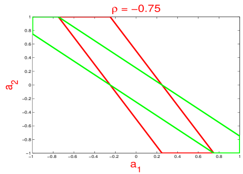
Figure 1: Let $C_{SS}$ and $\beta_{S}$ be as in Section 2.3.2, where $\rho=-0.75$. For a row of $C_{NS}$, say, $(a_{1},a_{2})$. The interior of the red box and that of the green box are the regions of $(a_{1},a_{2})$ satisfying the condition for the lasso (i.e. (12)) and for marginal regression (i.e. (13)), respectively.

2.3.3 In the special case of $C_{SS}=I$, the condition for the lasso is weaker

Fix $n$ and consider the special case in which $C_{SS}=I$. For the lasso, Condition E’ (and thus E) is satisfied, Condition J’ reduces to $\lambda<\rho$, and Condition I becomes $\|C_{NS}\|\leq 1$. Under these conditions, the lasso gives exact reconstruction, but Condition F can fail. To see how, let $\widetilde{\beta}\in\{-1,1\}^{s}$ be the vector such that $\max|C_{NS}\widetilde{\beta}|=\|C_{NS}\|_{\infty}$ and let $\ell$ be the index of the row at which the maximum is attained, choosing the row with the biggest absolute element if the maximum is not unique. Let $u$ be the maximum absolute element of row $\ell$ of $C_{NS}$ with index $j$. Define a vector $\delta$ to be zero except in component $j$, which has the value $\rho\widetilde{\beta}_{j}/(u\|C_{NS}\|_{\infty})$. Let $\beta=\rho\widetilde{\beta}+\rho\delta$. Then,

$$|(C_{NS}\beta)_{\ell}| =\rho|(C_{NS}\widetilde{\beta})_{\ell}|+\rho\frac{1}{\|C_{NS}\|_{\infty}}$$ (16)

$$=\rho\left(\|C_{NS}\|_{\infty}+\frac{1}{\|C_{NS}\|_{\infty}}\right)$$ (17)

$$>\rho.$$ (18)

It follows that $\max|C_{NS}\beta|>\rho=\min|\beta|$, so Condition F fails.

On the other hand, suppose Condition F holds for all $\beta_{S}\in\{-1,1\}^{s}$. (It cannot hold for all $\mathcal{M}_{\rho}$ by Theorem 2). Then, for all $\beta_{S}\in\{-1,1\}^{s}$, $\max|C_{NS}\beta_{S}|\leq 1$, which implies that $\|C_{NS}\|_{\infty}\leq 1$. Choosing $\lambda<\rho$, we have Conditions E’, I, and J’ satisfied, showing by Theorem 1 that the lasso gives exact reconstruction.

It follows that the conditions for the lasso are weaker in this case.

2.3.4 Small eigenvalues of $(X_{S}^{\prime}X_{S})$ may have an adverse effect on the performance of the lasso, but not always on that for marginal regression

For simplicity, assume

$$\beta_{S}\propto 1_{S}.$$

(We remark that the phenomenon to be described below is not limited to the case of $\beta_{S}\propto 1_{S}$). For $1\leq i\leq s$, let $\lambda_{i}$ and $\xi_{i}$ be the $i$-th eigenvalue and eigenvector of $C_{SS}$. Without loss of generality, we assume that $\xi_{i}$ have unit $\ell^{2}$ norm. By elementary algebra, there are constants $a_{1},\ldots,a_{s}$ such that $1_{S}=c_{1}\xi_{1}+c_{2}\xi_{2}+\ldots+c_{s}\xi_{s}$. It follows

$$C_{SS}^{-1}\cdot 1_{S}=\sum_{i=1}^{s}\frac{c_{i}}{\lambda_{i}}\xi_{i}\qquad\mbox{and}\qquad C_{SS}\cdot 1_{S}=\sum_{i=1}^{s}(c_{i}\lambda_{i})\xi_{i}.$$

Fix a row of $C_{NS}$, say, $a=(a_{1},\ldots,a_{s})$. Respectively, the conditions for the lasso and marginal regression require

$$|(a,\sum_{i=1}^{s}\frac{c_{i}}{\lambda_{i}}\xi_{i})|\leq 1\qquad\mbox{and}\qquad|(a,1_{S})|\leq|\sum_{i=1}^{s}(c_{i}\lambda_{i})\xi_{i}|.$$ (19)

Without loss of generality, we assume that $\lambda_{1}$ is the smallest eigenvalue of $C_{SS}$. Consider the case where $\lambda_{1}$ is small, while all other eigenvalues have a magnitude comparable to $1$. In this case, the smallness of $\lambda_{1}$ has a negligible effect on $\sum_{i=1}^{s}(c_{i}\lambda_{i})\xi_{i}$, and so has a negligible effect on the condition for marginal regression. However, the smallness of $\lambda_{1}$ may have an adverse effect on the performance of the lasso. To see the point, we note that $\sum_{i=1}^{s}\frac{c_{i}}{\lambda_{i}}\xi_{i}\approx\frac{c_{1}}{\lambda_{1}}\xi_{1}$. Compare this with the first term in (19). The condition for the lasso is roughly

$$|(a,\xi_{1})|\leq\lambda_{1},$$

which is rather restrictive since $\lambda_{1}$ is small.

We now further illustrate the point with an example. Let

$$C_{SS}=\left(\begin{array}[]{ccc}1&-1/2&c\\ -1/2&1&0\\ c&0&1\end{array}\right).$$

The smallest eigenvalue of the matrix is $\lambda_{1}=\lambda_{1}(c)=1-\sqrt{c^{2}+1/4}$, which is positive if and only if $c\leq\sqrt{3}/2$. Suppose $0<c<\sqrt{3}/2$. Fix a row of $C_{NS}$, say, $a=(a_{1},a_{2},a_{3})$. By direct calculations, the condition for marginal regression and the lasso require

$$|a_{1}+a_{2}+a_{3}|\leq 1/2,\;\mbox{and}\;|(6-4c)a_{1}+(6-3c-4c^{2})a_{2}+(3-6c)a_{3}|\leq(3-4c^{2})$$ (20)

respectively. As $c$ approaches $\sqrt{3}/2$, both $\lambda_{1}(c)$ and the right hand side of the first inequality in (20) approach $0$. As a result, the first inequality in (20) becomes increasingly more restrictive, but the the second inequality remains the same for all $c$. Therefore, a small $\lambda_{1}(c)$ has a negative effect on the broadness of the condition for the lasso, but not on that of marginal regression.

Figure 2 displays the regions where the vector $a$ satisfies the first and the second inequality in (20), respectively. In this example, $c=0.55,0.75,0.85$, so $\lambda_{1}(c)=0.29,0.14,0.014$ correspondingly. To better visualize these regions, we display their 2-D section in Figure 2 (in the 2-D section, we set the first coordinate of $a$ to $0$). The figures suggest that when $\lambda_{1}(c)$ get increasingly smaller, the region corresponding to the lasso shrinks substantially, while that corresponding to marginal regression remains the same.

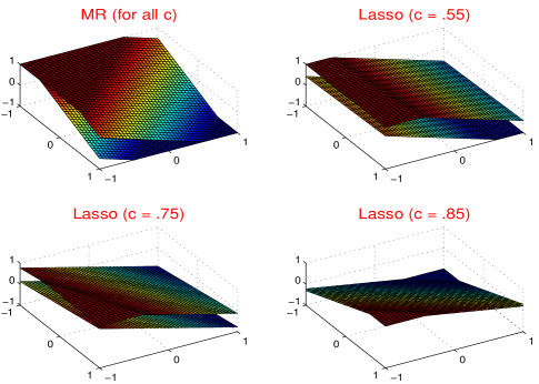
Figure 2: The regions sandwiched by two hyper-planes are the regions of $a=(a_{1},a_{2},a_{3})$ satisfying the condition for marginal regression (first inequality in (20); Panel 1) and for the lasso (second inequality of (20; Panel 2–4). Details of the example are in Section 2.3.4. Here, $c=0.55,0.75,0.85$ and the smallest eigenvalues of $C_{SS}$ are $\lambda_{1}(c)=0.29,0.14,0.014$. As $c$ varies, the regions for marginal regression remain the same so is displayed only in Panel 1 (MR stands for marginal regression). In contrast, the regions for the lasso get substantially smaller as $\lambda_{1}(c)$ decreases.

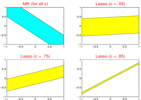
Figure 3: Displayed are the 2-D sections of the regions in Figure 2, where we set the first coordinate of $a$ to $0$. As $c$ varies, the regions for marginal regression remain the same, but those for the lasso get substantially smaller as $\lambda_{1}(c)$ decrease. $x$-axis: $a_{2}$. $y$-axis: $a_{3}$.

In conclusion, in the noise-free case, the condition for the lasso and for marginal regression are generally overlapping and closely related. On one hand, given a fixed matrix $X$, the conditions for the success of the lasso hold over a larger class of $\beta$’s than that of marginal regression. On the other hand, marginal regression has a larger tolerance for collinearity than does the lasso. Bear in mind that for very large $p$, the lasso is computationally much more demanding.

2.4 Exact reconstruction conditions for marginal regression in the noisy case

We now come back to Model (5) and consider the noisy case:

$$Y^{(n)}=X^{(n)}\beta^{(n)}+z^{(n)},\qquad\mbox{where}\qquad z^{(n)}\sim N(0,\sigma_{n}^{2}\cdot I_{n}).$$ (21)

To focus on variable selection, we suppose the parameter $\sigma_{n}^{2}$ is known. The exact reconstruction condition for the lasso in the noisy case has been studied extensively in the literature (see for example [26]). So in this paper, we focus on that for marginal regression. We address two topics. First, we extend Condition F in the noise-free case to the noisy case, say Condition F’. When Condition F’ holds, we show that with an appropriately chosen threshold $t$ (see (4)), marginal regression fully recovers the support with high probability. Second, we discuss how to determine the threshold $t$ empirically.

Recall that in the noise-free case, Condition F is

$$\max|C_{NS}\beta_{S}|\leq\min|C_{SS}\beta_{S}|.$$

A natural extension of Condition F is the following.

• Condition F’. (Faithfulness)

  $$\max|C_{NS}\beta_{S}|+2\sigma_{n}\sqrt{2\log p}\,<\,\min|C_{SS}\beta_{S}|.$$ (22)

When Condition F’ holds, it is possible to separate relevant variables from irrelevant variables with high probability. In detail, write

$$X=[x_{1},x_{2},\ldots,x_{p}],$$

where $x_{i}$ denotes the $i$-th column of $X$. Sort $|(Y,x_{i})|$ in the descending order, and let $r_{i}=r_{i}(Y,X)$ be the ranks of $|(Y,x_{i})|$ (assume no ties for simplicity). Introduce

$$\widehat{S}_{n}(k)=\widehat{S}_{n}(k;X,Y,p)=\{i:\;r_{i}(X,Y)\leq k\},\qquad k=1,2,\ldots,p.$$

Recall that $S(\beta)$ denotes the support of $\beta$ and $s=|S|$. The following lemma says that, if $s$ is known and Condition F’ holds, then marginal regression is able to fully recover the support $S$ with high probability.

Lemma 2.

Consider a sequence of regression models as in (21). If for sufficiently large $n$, Condition F’ holds and $p^{(n)}\geq n$, then

$$\lim_{n\rightarrow\infty}P\biggl{(}\widehat{S}_{n}(s^{(n)};X^{(n)},Y^{(n)},p^{(n)})\neq S(\beta^{(n)})\biggr{)}=0.$$

Lemma 2 is proved in the appendix. We remark that if both $s$ and $(p-s)$ tend to $\infty$ as $n$ tends to $\infty$, then Lemma 2 continues to hold if we replace $2\sigma_{n}\sqrt{2\log p}$ in (22) by $\sigma_{n}(\sqrt{\log(p-s)}+\sqrt{\log s})$. See the proof of the lemma for details.

The key assumption of Lemma 2 is that $s$ is known so that we know how to set the threshold $t$. Unfortunately, $s$ is generally unknown. We propose the following procedure to estimate $s$. Fix $1\leq k\leq p$, let $i_{k}$ be the unique index satisfying

$$r_{i_{k}}(X,Y)=k.$$

Let $\widehat{V}_{n}(k)=\widehat{V}_{n}(k;X,Y,p)$ be the linear space spanned by

$$x_{i_{1}},x_{i_{2}},\ldots,x_{i_{k}},$$

and let $\widehat{H}_{n}(k)=\widehat{H}_{n}(k;X,Y,p)$ be the projection matrix from $R^{n}$ to $\widehat{V}_{n}(k)$ (here and below, the $\widehat{\;}$ sign emphasizes the dependence of indices $i_{k}$ on the data). Define

$$\widehat{\delta}_{n}(k)=\widehat{\delta}_{n}(k;X,Y,p)=\|(\widehat{H}_{n}(k+1)-\widehat{H}_{n}(k))Y\|,\qquad 1\leq k\leq p-1.$$

The term $\widehat{\delta}_{n}^{2}(k)$ is closely related to the F-test for testing whether $\beta_{i_{k+1}}\neq 0$. We estimate $s$ by

$$\widehat{s}_{n}=\widehat{s}_{n}(X,Y,p)=\max\biggl{\{}1\leq k\leq p:\;\widehat{\delta}_{n}(k)\geq\sigma_{n}\sqrt{2\log n}\biggr{\}}+1$$

(in the case where $\widehat{\delta}(k)<\sigma_{n}\sqrt{2\log n}$ for all $k$, we define $\widehat{s}_{n}=1$).

Once $\widehat{s}_{n}$ is determined, we estimate the support $S$ by

$$\widehat{S}(\widehat{s}_{n},X,Y,p)=\{i_{k}:\,k=1,2,\ldots,\widehat{s}_{n}\}.$$

It turns out that under mild conditions, $\widehat{s}_{n}=s$ with high probability. In detail, suppose that the support $S(\beta)$ consists of indices $j_{1},j_{2},\ldots,j_{s}$. Fix $1\leq k\leq s$. Let $\widetilde{V}_{S}$ be the linear space spanned by $x_{j_{1}},\ldots,x_{j_{s}}$, and let $\widetilde{V}_{S,(-k)}$ be the linear space spanned by $x_{j_{1}},\ldots,x_{j_{k-1}},x_{j_{k+1}},\ldots,x_{j_{s}}$. Project $\beta_{j_{k}}x_{j_{k}}$ to the linear space $\widetilde{V}_{S}\cap\widetilde{V}_{S,(-k)}^{\perp}$. Let $\Delta_{n}(k,\beta,X,p)$ be the $\ell^{2}$ norm of the resulting vector, and let

$$\Delta_{n}^{*}(\beta,X,p)=\min_{1\leq k\leq s}\Delta_{n}(k,\beta,X,p).$$

The following theorem says that if $\Delta_{n}^{*}(\beta,X,p)$ is slightly larger than $\sigma_{n}\sqrt{2\log n}$, then $\widehat{s}_{n}=s$ and $\widehat{S}_{n}=S$ with high probability. In other words, marginal regression fully recovers the support with high probability. Theorem 3 is proved in the appendix.

Theorem 3.

Consider a sequence of regression models as in (21). Suppose that for sufficiently large $n$, Condition F’ holds, $p^{(n)}\geq n$, and

$$\lim_{n\rightarrow\infty}\biggl{(}\frac{\Delta_{n}^{*}(\beta^{(n)},X^{(n)},p^{(n)})}{\sigma_{n}}-\sqrt{2\log n}\biggr{)}=\infty.$$

Then

$$\lim_{n\rightarrow\infty}P\biggl{(}\widehat{s}_{n}(X^{(n)},Y^{(n)},p^{(n)})\neq s^{(n)}\biggr{)}\rightarrow 0,$$

and

$$\lim_{n\rightarrow\infty}\biggl{(}\widehat{S}_{n}(\widehat{s}_{n}(X^{(n)},Y^{(n)},p^{(n)});X^{(n)},Y^{(n)},n,p^{(n)})\neq S(\beta^{(n)})\biggr{)}\rightarrow 0.$$

Theorem 3 says that the tuning parameter for marginal regression (i.e. the threshold $t$) can be set successfully in a data driven fashion. In comparison, how to set the tuning parameter $\lambda$ for the lasso has been a withstanding open problem in the literature.

3 The Deterministic Design, Random Coefficient Regime

Recall that the Faithfulness Condition is

$$\max|C_{NS}\beta_{S}|\leq\min|C_{SS}\beta_{S}|.$$

In this section, we study how broad the Faithfulness Condition holds. We approach this by modeling $\beta$ as random (the matrix $X$ is kept deterministic), and find out conditions under which the Faithfulness Condition holds with high probability.

The discussion in this section is closely related to the work by Donoho and Elad [8] on the Incoherence Condition. Compared to the Faithfulness Condition, the advantage of the Incoherence Condition is that it does not involve the unknown support of $\beta$, so it is checkable in practice. The downside of the Incoherence Condition is that it aims to control the worst case so it is conservative. In this section, we derive a condition—Condition F”— which can be viewed as a middle ground between the Faithfulness Condition and the Incoherence Condition: it is not tied to the unknown support so it is more tractable than the Faithfulness Condition, and it is also much less stringent than the Incoherence Condition.

In detail, we model $\beta$ as follows. Fix $\epsilon\in(0,1)$, $a>0$, and a distribution $\pi$, where

$$\mbox{the support of $\pi$}\qquad\subset\qquad(-\infty,-a]\cup[a,\infty).$$ (23)

For each $1\leq i\leq p$, we draw a sample $B_{i}$ from $\mathrm{Bernoulli}(\epsilon)$. When $B_{i}=0$, we set $\beta_{i}=0$. When $B_{i}=1$, we draw $\beta_{i}\sim\pi$. Marginally,

$$\beta_{i}\stackrel{{\scriptstyle iid}}{{\sim}}(1-\epsilon)\nu_{0}+\epsilon\pi,$$ (24)

where $\nu_{0}$ denotes the point mass at $0$. We study for which quadruplets $(X,\epsilon,\pi,a)$ the Faithfulness Condition holds with high probability.

Recall that the design matrix $X=[x_{1},\ldots,x_{p}]$, where $x_{i}$ denotes the $i$-th column. Fix $t\geq 0$ and $\delta>0$. Introduce

$$g_{ij}(t)=E_{\pi}[e^{tu(x_{i},x_{j})}]-1,\qquad\bar{g}_{i}(t)=\sum_{j\neq i}g_{ij}(t),$$

where the random variable $u\sim\pi$. As before, we have suppressed the superscript $\,{}^{(n)}$ for $g_{ij}(t)$ and $\bar{g}_{i}(t)$. Define

$$A_{n}(\delta,\epsilon,\bar{g})=A_{n}(\delta,\epsilon,\bar{g};X,\pi)=\min_{t>0}\biggl{(}e^{-\delta t}\sum_{i=1}^{p}[e^{\epsilon\bar{g}_{i}(t)}+e^{\epsilon\bar{g}_{i}(-t)}]\biggr{)},$$

where $\bar{g}$ denotes the vector $(\bar{g}_{1},\ldots,\bar{g}_{p})^{T}$. The following lemma is proved in the appendix.

Lemma 3.

Fix $n$, $X$, $\delta>0$, $\epsilon\in(0,1)$, and distribution $\pi$. Then

$$P(\max|C_{NS}\beta_{S}|\geq\delta)\leq(1-\epsilon)A_{n}(\delta,\epsilon,\bar{g};X,\pi),$$ (25)

and

$$\qquad P(\max|(C_{SS}-I_{S})\beta_{S}|\geq\delta)\leq\epsilon A_{n}(\delta,\epsilon,\bar{g};X,\pi).$$ (26)

Now, suppose the distribution $\pi$ satisfies (23) for some $a>0$. Take $\delta=a/2$ on the right hand side of (25)-(26). Except for a probability of $A_{n}(a/2,\epsilon,\bar{g})$,

$$\max|C_{NS}\beta_{S}|\leq a/2,\qquad\min|C_{SS}\beta_{S}|\geq\min|\beta_{S}|-\max|(C_{SS}-I)\beta_{S}|\geq a/2,$$

so $\max|C_{NS}\beta_{S}|\leq\min|C_{SS}\beta_{S}|$ and the Faithfulness Condition holds. This motivates the following condition, where $(a,\epsilon,\pi)$ may depend on $n$.

• Condition F”. (Faithfulness)

  $$\lim_{n\rightarrow\infty}A_{n}(a_{n}/2,\epsilon_{n},\bar{g}^{(n)};X^{(n)},\pi_{n})=0.$$ (27)

The following theorem says that if Condition F” holds, then Condition F holds with high probability.

Theorem 4.

Consider a sequence of noise-free regression models as in (21), where the noise component $z^{(n)}=0$ and $\beta^{(n)}$ is generated as in (24). Suppose Condition F” holds. Then as $n$ tends to $\infty$, except for a probability that tends to $0$,

$$\max|C_{NS}\beta_{S}|\leq\min|C_{SS}\beta_{S}|.$$

Theorem 4 is the direct result of Lemma 3 so we omit the proof.

3.1 Comparison of Condition F” with the Incoherence Condition

Introduced in Donoho and Elad [8] (see also [9]), the Incoherence of a matrix $X$ is defined as [8]

$$\max_{i\neq j}|C_{ij}|,$$

where $C=X^{T}X$ is the Gram matrix as before. The notion is motivated by the study in recovering a sparse signal from an over-complete dictionary. In the special case where $X$ is the concatenation two orthonormal bases (e.g. a Fourier basis and a wavelet basis), $\max_{i\neq j}|C_{ij}|$ measures how coherent two bases are and so the term of incoherence; see [8, 9] for details. Consider Model (1) in the case where both $X$ and $\beta$ are deterministic, and the noise component $z=0$. The following results are proved in [5, 8, 9].

• Lasso yields exact variable selection if $s<\frac{1+\max_{i\neq j}|C_{ij}|}{2\max_{i\neq j}|C_{ij}|}$.

• Marginal regression yields exact variable selection if $s<\frac{c}{2\max_{i\neq j}|C_{ij}|}$ for some constant $c\in(0,1)$, and that the nonzero coordinates of $\beta$ have comparable magnitudes (i.e. the ratio between the largest and the smallest nonzero coordinate of $\beta$ is bounded away from $\infty$).

In comparison, the Incoherence Condition only depends on $X$ so it is checkable. Condition F depends on the unknown support of $\beta$. Checking such a condition is almost as hard as estimating the support $S$. Condition F” provides a middle ground. It depends on $\beta$ only through $(\epsilon,\pi)$. In cases where we either have a good knowledge of $(\epsilon,\pi)$ or we can estimate them, Condition F” is checkable.

At the same time, the Incoherence Condition is conservative, especially when $s$ is large. In fact, in order for either the lasso or marginal regression to have an exact variable selection, it is required that

$$\max_{i\neq j}|C_{ij}|\leq O\biggl{(}\frac{1}{s}\biggr{)},$$ (28)

In other words, all coordinates of the Gram matrix $C$ need to be no greater than $O(1/s)$. This is much more conservative than Condition F.

However, we must note that the Incoherence Condition aims to control the worst case: it sets out to guarantee uniform success of a procedure across all $\beta$ under minimum constraints. In comparison, Condition F aims to control a single case, and Condition F” aims to control almost all the cases in a specified class. As such, Condition F” provides a middle ground between Condition F and the Incoherence Condition, applying more broadly than the former, while being less conservative than the later.

Below, we use two examples to illustrate that Condition F” is much less conservative than the Incoherence Condition. In the first example, we consider a weakly dependent case where $\max_{i\neq j}|C_{ij}|\leq O(1/\log(p))$. In the second example, we suppose the matrix $C$ is sparse, but the nonzero coordinates of $C$ may be large.

3.1.1 The weakly dependent case

Suppose that for sufficiently large $n$, there are two sequence of positive numbers $a_{n}\leq b_{n}$ such that

$$\mbox{the support of $\pi_{n}$}\qquad\subset\qquad[-b_{n},-a_{n}]\cup[a_{n},b_{n}],$$

and that

$$\frac{b_{n}}{a_{n}}\cdot\max_{i\neq j}|C_{ij}|\leq c_{1}/\log(p),\qquad\mbox{$c_{1}>0$ is a constant}.$$

For $k\geq 1$, denote the $k$-th moment of $\pi_{n}$ by

$$\mu_{n}^{(k)}=\mu_{n}^{(k)}(\pi_{n}).$$ (29)

Introduce $m_{n}=m_{n}(X)$ and $v_{n}^{2}=v_{n}^{2}(X)$ by

$$m_{n}(X)=p\epsilon_{n}\cdot\max_{1\leq i\leq p}\biggl{\{}\biggl{|}\frac{1}{p}\sum_{j\neq i}C_{ij}\biggr{|}\biggr{\}},\qquad v_{n}^{2}(X)=p\epsilon_{n}\cdot\max_{1\leq i\leq p}\biggl{\{}\frac{1}{p}\sum_{j\neq i}C^{2}_{ij}\biggr{\}}.$$

Corollary 3.1.

Consider a sequence of regression models as in (21), where the noise component $z^{(n)}=0$ and $\beta^{(n)}$ is generated as in (24). If there are constants $c_{1}>0$ and $c_{2}\in(0,1/2)$ such that

$$\frac{b_{n}}{a_{n}}\cdot\max_{i\neq j}\{|C_{ij}|\}\leq c_{1}/\log(p^{(n)}),$$

and

$$\mathop{\overline{\rm lim}}_{n\rightarrow\infty}\biggl{(}\frac{\mu_{n}^{(1)}(\pi_{n})}{a_{n}}m_{n}(X^{(n)})\biggr{)}\leq c_{2},\qquad\mathop{\overline{\rm lim}}_{n\rightarrow\infty}\biggl{(}\frac{\mu_{n}^{(2)}(\pi_{n})}{a_{n}^{2}}v_{n}^{2}(X^{(n)})\log(p^{(n)})\biggr{)}=0,$$ (30)

then

$$\lim_{n\rightarrow\infty}A_{n}(a_{n}/2,\epsilon_{n},\bar{g}^{(n)};X^{(n)},\pi_{n})=0,$$

and Condition F” holds.

Corollary 3.1 is proved in the appendix. For interpretation, we consider the special case where there is a generic constant $c>0$ such that $b_{n}\leq ca_{n}$. As a result, $\mu_{n}^{(1)}/a_{n}\leq c$, $\mu_{n}^{(2)}/a_{n}^{2}\leq c^{2}$. The conditions reduce to that, for sufficiently large $n$ and all $1\leq i\leq p$,

$$|\frac{1}{p}\sum_{j\neq i}^{p}C_{ij}|\leq O(\frac{1}{p\epsilon_{n}}),\qquad\frac{1}{p}\sum_{j\neq i}^{p}C^{2}_{ij}=o(1/p\epsilon_{n}).$$

Note that by (24), $s=s^{(n)}\sim\mathrm{Binomial}(p,\epsilon_{n})$, so $s\approx p\epsilon_{n}$. Recall that the Incoherence Condition is

$$\max_{i\neq j}|C_{ij}|\leq O(1/s).$$

In comparison, the Incoherence Condition requires that each coordinate of $(C-I)$ is no greater than $O(1/s)$, while Condition F” only requires that the average of each row of $(C-I)$ is no greater than $O(1/s)$. The latter is much less conservative.

3.1.2 The sparse case

Let $N_{n}^{*}(C)$ be the maximum number of nonzero off-diagonal coordinates of $C$:

$$N_{n}^{*}(C)=\max_{1\leq i\leq p}\{N_{n}(i)\},\qquad N_{n}(i)=N_{n}(i;C)=\#\{j:\;j\neq i,C_{ij}\neq 0\}.$$

Suppose there is a constant $c_{3}>0$ such that

$$\mathop{\underline{\rm lim}}_{n\rightarrow\infty}\biggl{(}\frac{-\log(\epsilon_{n}N_{n}^{*}(C))}{\log(p^{(n)})}\biggr{)}\geq c_{3}.$$ (31)

Also, suppose there is a constant $c_{4}>0$ such that for sufficiently large $n$,

$$\mbox{the support of $\pi_{n}$ is contained in $[-c_{4}a_{n},a_{n}]\cup[a_{n},c_{4}b_{n}]$}.$$ (32)

The following corollary is proved in the appendix.

Corollary 3.2.

Consider a sequence of noise-free regression models as in (21), where the noise component $z^{(n)}=0$ and $\beta^{(n)}$ is randomly generated as in (24). Suppose (31)-(32) hold. If there is a constant $\delta>0$ such that

$$\max_{i\neq j}|C_{ij}|\leq\delta,\qquad\mbox{and}\qquad\delta<\frac{c_{3}}{2c_{4}},$$ (33)

then

$$\lim_{n\rightarrow\infty}A_{n}(a_{n}/2,\epsilon_{n},\bar{g}^{(n)};X^{(n)},\pi_{n})=0,$$

and Condition F” holds.

For interpretation, consider a special case where

$$\epsilon_{n}=p^{-\vartheta}.$$

In this case, the condition reduces to

$$N_{n}^{*}(C)\ll p^{\vartheta-2c_{4}\delta}.$$

As a result, Condition F” is satisfied if each row of $(C-I)$ contains no more than $p^{\vartheta-2c_{4}\delta}$ nonzero coordinates each of which $\leq\delta$. Compared to the Incoherence Condition $\max_{i\neq j}|C_{ij}|\leq O(1/s)=O(p^{-\vartheta})$, our condition is much weaker.

In conclusion, if we alter our attention from the worst-case scenario to the average scenario, and alter our aim from exact variable selection to exact variable selection with probability $\approx 1$, then the condition required for success—Condition F”—is much more relaxed than the Incoherence Condition.

4 Hamming Distance when $X$ is Gaussian; Partition of the Phase Diagram

So far, we have focused on exact variable selection. In many applications, exact variable selection is not possible. Therefore, it is of interest to study the Type I and Type II errors of variable selection (a Type I error is a misclassified $0$ coordinate of $\beta$, and a Type II error is a misclassified nonzero coordinate).

In this section, we use the Hamming distance to measure the variable selection errors. Back to Model (1),

$$Y=X\beta+z,\qquad z\sim N(0,I_{n}),$$ (34)

where without loss of generality, we assume $\sigma_{n}=1$. As in the preceding section (i.e. (24)), we suppose

$$\beta_{i}\stackrel{{\scriptstyle iid}}{{\sim}}(1-\epsilon)\nu_{0}+\epsilon\pi.$$ (35)

For any variable selection procedure $\widehat{\beta}=\widehat{\beta}(Y;X)$, the Hamming distance between $\widehat{\beta}$ and the true $\beta$ is

$$d(\widehat{\beta}|X)=d(\widehat{\beta};\epsilon,\pi|X)=\sum_{j=1}^{p}E_{\epsilon,\pi}(E_{z}[1(\mathop{\rm sgn}(\widehat{\beta}_{j})\neq\mathop{\rm sgn}(\beta_{j}))|X]).$$

Note that by Chebyshev’s inequality,

$$P(\mbox{non-exact variable selection by $\widehat{\beta}(Y;X)$})\leq d(\widehat{\beta}|X).$$

So a small Hamming distance guarantees exact variable selection with high probability.

How to characterize precisely the Hamming distance is a challenging problem. We approach this by modeling $X$ as random. Assume that the coordinates of $X$ are iid samples from $N(0,1/n)$:

$$X_{ij}\stackrel{{\scriptstyle iid}}{{\sim}}N(0,1/n).$$ (36)

The choice of the variance ensures that most diagonal coordinates of the Gram matrix $C=X^{T}X$ are approximately $1$. Let $P_{X}(x)$ denote the joint density of the coordinates of $X$. The expected Hamming distance is then

$$d^{*}(\widehat{\beta})=d^{*}(\widehat{\beta};\epsilon,\pi)=\int d(\widehat{\beta};\epsilon,\pi|X=x)P_{X}(x)dx.$$

We adopt an asymptotic framework where we calibrate $p$ and $\epsilon$ with

$$p=n^{1/\theta},\qquad\epsilon_{n}=n^{(1-\vartheta)/\theta}\equiv p^{1-\vartheta},\qquad 0<\theta,\vartheta<1.$$ (37)

This models a situation where $p\gg n$ and the vector $\beta$ gets increasingly sparse as $n$ grows. Also, we assume $\pi_{n}$ in (24) is a point mass

$$\pi_{n}=\nu_{\tau_{n}}.$$ (38)

Despite its seemingly idealistic, the model was found to be subtle and rich in theory (e.g. [2, 10, 12, 11, 20, 22]). In addition, compare two experiments, in one of them $\pi_{n}=\nu_{\tau_{n}}$, and in the other the support of $\pi_{n}$ is contained in $[\tau_{n},\infty)$. Since the second model is easier for inference than the first one, the optimal Hamming distance for the first one gives an upper bound for that for the second one.

With $\epsilon_{n}$ calibrated as above, the most interesting range for $\tau_{n}$ is $O(\sqrt{2\log p})$ [10]: when $\tau_{n}\gg\sqrt{2\log p}$, exact variable selection can be easily achieved by either the lasso or marginal regression. When $\tau_{n}\ll\sqrt{2\log p}$, no variable selection procedure can achieve exact variable selection. In light of this, we calibrate

$$\tau_{n}=\sqrt{2(r/\theta)\log n}\equiv\sqrt{2r\log p},\qquad r>0.$$ (39)

With these calibrations, we can rewrite

$$d_{n}^{*}(\widehat{\beta};\epsilon,\pi)=d_{n}^{*}(\widehat{\beta};\epsilon_{n},\tau_{n}).$$

Definition 4.1.

Denote $L(n)$ by a multi-log term which satisfies that $\lim_{n\rightarrow\infty}(L(n)\cdot n^{\delta})=\infty$ and that $\lim_{n\rightarrow\infty}(L(n)\cdot n^{-\delta})=0$ for any $\delta>0$.

We are now ready to spell out the main results. Define

$$\rho(\vartheta)=(1+\sqrt{1-\vartheta})^{2},\qquad 0<\vartheta<1.$$

The following theorem is proved in the appendix, which gives the lower bound for the Hamming distance.

Theorem 5.

Fix $\vartheta\in(0,1)$, $\theta>0$, and $r>0$ such that $\theta>2(1-\vartheta)$. Consider a sequence of regression models as in (34)-(39). As $n\rightarrow\infty$, for any variable selection procedure $\widehat{\beta}^{(n)}$,

$$d_{n}^{*}(\widehat{\beta}^{(n)};\epsilon_{n},\tau_{n})\geq\left\{\begin{array}[]{ll}L(n)p^{1-\frac{(\vartheta+r)^{2}}{4r}},&\qquad r\geq\vartheta,\\ (1+o(1))\cdot p^{1-\vartheta},&\qquad 0<r<\vartheta.\end{array}\right.$$

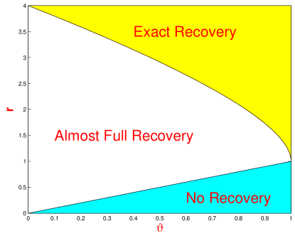
Figure 4: There regions as in Section 4. In Region of Exact Recovery, both the lasso and marginal regression yield exact recovery with high probability. In Region of Almost Full Recovery, it is impossible to have large probability for exact variable selection, but the Hamming distance of both the lasso and marginal regression $\ll p\epsilon_{n}$. In Region of No Recovery, optimal Hamming distance $\sim p\epsilon_{n}$ and all variable selection procedures fail completely. Displayed is the part of the plane corresponding to $0<r<4$ only.

At the same time, let $\widehat{\beta}_{mr}$ be the estimate of using marginal regression with threshold

$$t_{n}=(\frac{\vartheta+r}{2\sqrt{r}}\wedge\sqrt{r})\cdot\sqrt{2\log p}.$$

We have the following theorem.

Theorem 6.

Fix $\vartheta\in(0,1)$, $r>0$, and $\theta>(1-\vartheta)$. Consider a sequence of regression models as in (34)-(39). As $p\rightarrow\infty$, the Hamming distance of marginal regression with the threshold $t_{n}=(\frac{\vartheta+r}{2\sqrt{r}}\wedge\sqrt{r})\cdot\sqrt{2\log p^{(n)}}$ satisfies

$$d_{n}^{*}(\widehat{\beta}_{mr}^{(n)};\epsilon_{n},\tau_{n})\leq\left\{\begin{array}[]{ll}L(n)p^{1-\frac{(\vartheta+r)^{2}}{4r}},&\qquad r\geq\vartheta,\\ (1+o(1))\cdot p^{1-\vartheta},&\qquad 0<r<\vartheta.\end{array}\right.$$

Similarly, choosing the tuning parameter $\lambda_{n}=2(\frac{\vartheta+r}{2\sqrt{r}}\wedge\sqrt{r})\sqrt{2\log p}$ in the lasso, we have the following theorem.

Theorem 7.

Fix $\vartheta\in(0,1)$, $r>0$, and $\theta>(1-\vartheta)$. Consider a sequence of regression models as in (34)-(39). As $p\rightarrow\infty$, the Hamming distance of the lasso with the tuning parameter $\lambda_{n}=2(\frac{\vartheta+r}{2\sqrt{r}}\wedge\sqrt{r})\cdot\sqrt{2\log p^{(n)}}$ satisfies

$$d_{n}^{*}(\widehat{\beta}_{lasso}^{(n)};\epsilon_{n},\tau_{n})\leq\left\{\begin{array}[]{ll}L(n)p^{1-\frac{(\vartheta+r)^{2}}{4r}},&\qquad r\geq\vartheta,\\ (1+o(1))\cdot p^{1-\vartheta},&\qquad 0<r<\vartheta.\end{array}\right.$$

The proofs of Theorems 6-7 are routine and we omit them.

Theorems 5-7 say that in the $\vartheta$-$r$ plane, we have three different regions, as displayed in Figure 4.

• Region I (Exact Reovery): $0<\vartheta<1$ and $r>\rho(\vartheta)$.

• Region II (Almost Full Recovery): $0<\vartheta<1$ and $\vartheta<r<\rho(\vartheta)$.

• Region III (No Recovery): $0<\vartheta<1$ and $0<r<\vartheta$.

In the Region of Exact Recovery, the Hamming distance for both marginal regression and the lasso are algebraically small. Therefore, except for a probability that is algebraically small, both marginal regression and the lasso give exact recovery.

In the Region of Almost Full Recovery, both the Hamming distance of marginal regression and the lasso are much smaller than the number of relevant variables (which $\approx p\epsilon_{n}$). Therefore, almost all relevant variables have been recovered. Note also that the number of misclassified irrelevant variables is comparably much smaller than $p\epsilon_{n}$. In this region, the optimal Hamming is algebraically large, so for any variable selection procedure, the probability of exact recovery is algebraically small.

In the Region of No Recovery, the Hamming distance $\sim p\epsilon_{n}$. In this region, asymptotically, it is impossible to distinguish relevant variables from irrelevant variables, and any variable selection procedure fails completely.

The results improve on those by Wainwright [30]. It was shown in [30] that there are constants $c_{2}>c_{1}>0$ such that in the region of $\{0<\vartheta<1,r>c_{2}\}$, the lasso yields exact variable selection with overwhelming probability, and that in the region of $\{0<\vartheta<1,r<c_{2}\}$, no procedure could yield exact variable selection. Our results not only provide the exact rate of the Hamming distance, but also tighten the constants $c_{1}$ and $c_{2}$ so that $c_{1}=c_{2}=(1+\sqrt{1-\vartheta})^{2}$.

5 Simulations and Examples

In this section we consider some numerical examples. Figures 5 and 6 show the prediction error and the Hamming error for the lasso and marginal regression, as a function of the number of variables selected. In all cases, $n=40$, $p=500$, $\sigma=10$ and $s=100$. All nonzero $\beta_{j}$’s are set equal to either $.5$ or 5. Each row of the matrix $X$ is generated independently from $N(0,\Sigma(\rho))$, where $\Sigma(\rho)$ is a $p$ by $p$ matrix with $1$ on the diagonal and $\rho$ elsewhere. We take $\rho=0,0.2,0.5,0.9$. Figures 7 and 8 are the same but are averaged over 100 replications.

We see that in virtually all cases, marginal regression is competitive with the lasso and in some cases is much better.

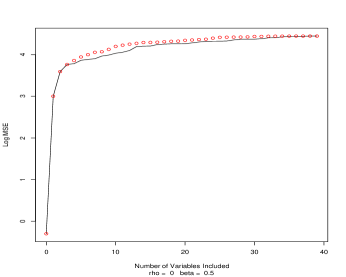
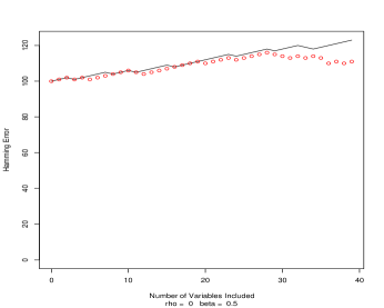
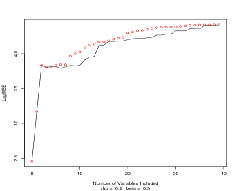
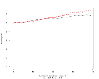
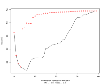
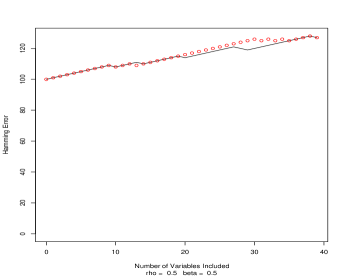
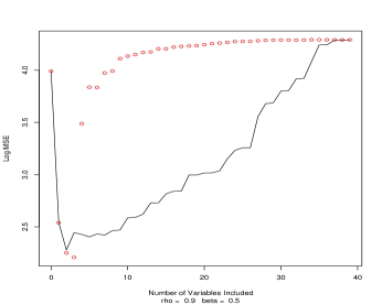
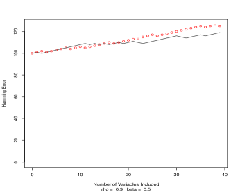
Figure 5: Prediction error (left column) and Hamming error (right column) for the lasso (red circle) and marginal regression (solid line). The x-axis displays the number of variables included. Row 1-4: $\rho=0,0.2,0.5,0.9$. Nonzero $\beta_{i}$: $0.5$. Results are based on one replication.

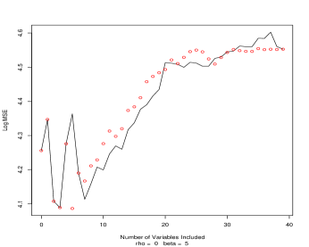
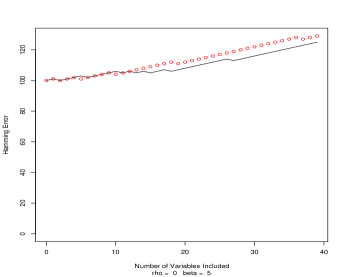
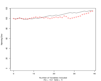
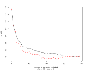
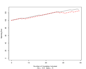
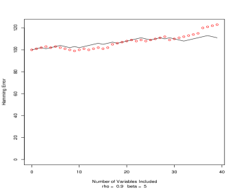
Figure 6: Same as in Figure 5, but all nonzero $\beta_{i}$ equal $5$.

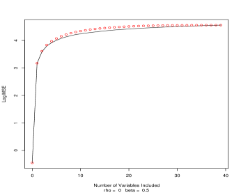
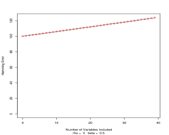
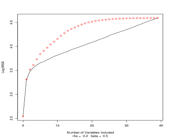
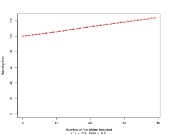
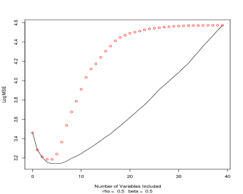
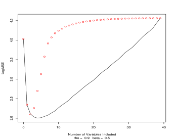
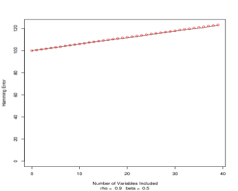
Figure 7: Same as in Figure 5, but displayed are the average errors across $100$ replications.

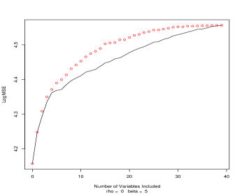
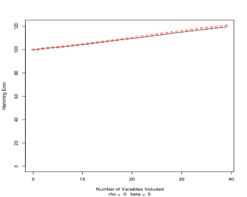
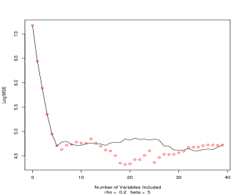
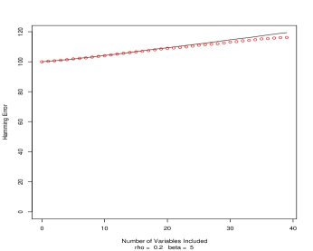
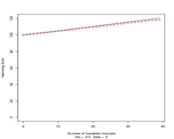
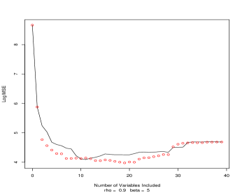
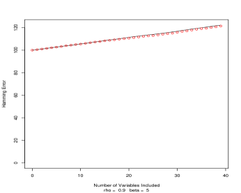
Figure 8: Same as in Figure 6, but displayed are the average errors across $100$ replications.

6 Proofs

6.1 Proof of Theorem 2

First, let $k_{i}$ denote the number of non-zero diagonal entries in row $i$ of $C$. Because $C$ is symmetric but not diagonal, at least two rows must have non-zero $k_{i}$. Assume without loss of generality that the rows and columns of $C$ are arranged so that the rows with non-zero $k_{i}$ form the initial minor. It follows that the initial minor is itself a positive definite symmetric matrix. And because any such matrix $A$ satisfies $|A_{ij}|<\max_{k}C_{kk}$ for $j\neq i$, there exists a row $i$ of $C$ with $k_{i}>0$ and $|C_{ij}|<C_{ii}$ for any $j\neq i$.

Define $\beta$ as follows:

$$\beta_{j}=\begin{cases}\frac{\rho C_{ii}}{C_{ij}}&\text{if $j\neq i$ and $C_{ij}\neq 0$}\\ \rho&\text{if $j\neq i$ and $C_{ij}=0$}\\ -k_{i}\rho&\text{if $j=i$.}.\end{cases}$$ (40)

Because $|C_{ij}|\leq C_{ii}$, this satisfies $|\beta_{j}|\geq\rho$, so $\beta\in\mathcal{M}^{s}_{\rho}$. Moreover,

$$(C\beta)_{i}=\sum_{j}C_{ij}\beta_{j}=-k_{i}C_{ii}\rho+\sum_{{j\neq i\atop C_{ij}\neq 0}}\frac{\rho C_{ii}}{C_{ij}}C_{ij}=0.$$ (41)

This proves the theorem.

6.2 Proof of Lemma 2

By the definition of $\widehat{S}_{n}(s)$, it is sufficient to show that except for a probability that tends to $0$,

$$\max|X_{N}^{T}Y|<\min|X_{S}^{T}Y|.$$

Since $Y=X\beta+z=X_{S}\beta_{S}+z$, we have $X_{N}^{T}Y=X_{N}^{T}(X_{S}\beta_{S}+z)=C_{NS}\beta_{S}+X_{N}^{T}z$. Note that $x_{i}^{T}z\sim N(0,\sigma_{n}^{2})$. By Boolean algebra and elementary statistics,

$$P(\max|X_{N}^{T}z|>\sigma_{n}\sqrt{2\log p})\leq\sum_{i\in N}P(|(x_{i},z)|\geq\sigma_{n}\sqrt{2\log p})\leq\frac{C}{\sqrt{\log p}}\frac{p-s}{p}.$$

It follows that except for a probability of $o(1)$,

$$\max|X_{N}^{T}Y|\leq\max|C_{NS}\beta_{S}|+\max|X_{N}^{T}z|\leq\max|C_{NS}\beta_{S}|+\sigma_{n}\sqrt{2\log p}.$$

Similarly, except for a probability of $o(1)$,

$$\min|X_{S}^{T}Y|\geq\min|C_{SS}\beta_{S}|-\max|X_{S}^{T}z|\geq\min|C_{SS}\beta_{S}|-\sigma_{n}\sqrt{2\log p}.$$

Combining these gives the claim.  $\;\;\scriptstyle\Box$

6.3 Proof of Theorem 3

Once the first claim is proved, the second claim follows from Lemma 2. So we only show the first claim. Write for short $\widehat{S}_{n}(s)=\widehat{S}_{n}(s^{(n)};X^{(n)},Y^{(n)},p^{(n)})$, $s=s^{(n)}$, and $S=S(\beta^{(n)})$. All we need to show is

$$\lim_{n\rightarrow\infty}P(\widehat{s}_{n}\neq s)=0.$$

Introduce the event

$$D_{n}=\{\widehat{S}_{n}(s)=S\}.$$

It follows from Lemma 2 that

$$P(D_{n}^{c})\rightarrow 0.$$

Write

$$P(\widehat{s}_{n}\neq s)\leq P(D_{n})P(\widehat{s}_{n}\neq s|D_{n})+P(D_{n}^{c}).$$

It is sufficient to show $\lim_{n\rightarrow\infty}P(\widehat{s}_{n}\neq s|D_{n})=0$, or equivalently,

$$\lim_{n\rightarrow\infty}P(\widehat{s}_{n}>s|D_{n})=0\qquad\mbox{and}\qquad\lim_{n\rightarrow\infty}P(\widehat{s}_{n}<s|D_{n})=0.$$ (42)

Consider the first claim of (42). Write for short $t_{n}=\sigma_{n}\sqrt{2\log n}$. Note that the event $\{\widehat{s}_{n}>s|D_{n}\}$ is contained in the event of $\cup_{k=s}^{p-1}\{\widehat{\delta}_{n}(k)\geq t_{n}|D_{n}\}$. Recalling $P(D_{n}^{c})=o(1)$,

$$P(\widehat{s}_{n}>s)\leq\sum_{k=s}^{p-1}(\widehat{\delta}(k)\geq t_{n}|D_{n})\lesssim\sum_{k=s}^{p-1}P(\widehat{\delta}_{n}(k)\geq t_{n}),$$ (43)

where we say two positive sequences $a_{n}\lesssim b_{n}$ if $\mathop{\overline{\rm lim}}_{n\rightarrow\infty}(a_{n}/b_{n})\leq 1$.

Fix $s\leq k\leq p-1$. By definitions, $\widehat{H}(k+1)-\widehat{H}(k)$ is the projection matrix from $R^{n}$ to $\widehat{V}_{n}(k+1)\cap\widehat{V}_{n}(k)^{\perp}$. So conditional on the event $\{\widehat{V}_{n}(k+1)=\widehat{V}_{n}(k)\}$, $\delta_{n}(k)=0$, and conditional on the event $\{\widehat{V}_{n}(k+1)\subsetneq\widehat{V}_{n}(k)\}$, $\delta_{n}^{2}(k)\sim\sigma_{n}^{2}\chi^{2}(1)$. Note that $P(\chi^{2}(1)\geq\ 2\log n)=o(1/n)$. It follows that

$$\sum_{k=s}^{p-1}P(\widehat{\delta}_{n}(k)\geq t_{n}) =\sum_{k=s}^{p-1}P(\widehat{\delta}_{n}(k)\geq t_{n}|\widehat{V}_{n}(k)\subsetneq\widehat{V}_{n}(k+1))P(\widehat{V}_{n}(k)\subsetneq\widehat{V}_{n}(k+1))$$

$$=o(\frac{1}{n})\sum_{k=s}^{p-1}P(\widehat{V}_{n}(k)\subsetneq\widehat{V}_{n}(k+1)).$$ (44)

Moreover,

$$\sum_{k=s}^{p-1}P(\widehat{V}_{n}(k)\subsetneq\widehat{V}_{n}(k+1)) =\sum_{k=s}^{p-1}E[1(\mathrm{dim}(\widehat{V}_{n}(k+1))>\mathrm{dim}(\widehat{V}_{n}(k)))]$$

$$=E[\sum_{k=s}^{p-1}1(\mathrm{dim}(\widehat{V}_{n}(k+1))>\mathrm{dim}(\widehat{V}_{n}(k)))].$$

Note that for any realization of the sequences $\widehat{V}_{n}(1),\ldots,\widehat{V}_{n}(p)$, $\sum_{k=s}^{p-1}1(\mathrm{dim}(\widehat{V}_{n}(k+1))>\mathrm{dim}(\widehat{V}_{n}(k)))\leq n$. It follows that

$$\sum_{k=s}^{p-1}P(\widehat{V}_{n}(k)\subsetneq\widehat{V}_{n}(k+1))\leq n.$$ (45)

Combining (43)-(45) gives the claim.

Consider the second claim of (42). By the definition of $\widehat{s}_{n}$, the event $\{\widehat{s}_{n}<s|D_{n})\}$ is contained in the event $\{\widehat{\delta}_{n}(s-1)<t_{n}|D_{n}\}$. By definitions, $\widehat{\delta}_{n}(s-1)=\|(\widehat{H}(s)-\widehat{H}(s-1))Y\|$, where $\|\cdot\|=\|\cdot\|_{2}$ denotes the $\ell^{2}$ norm. So all we need to show is

$$\lim_{n\rightarrow\infty}P(\|(\widehat{H}(s)-\widehat{H}(s-1))Y\|<t_{n}|D_{n})=0.$$ (46)

Fix $1\leq k\leq p$. Recall that $i_{k}$ denotes the index at which the rank of $|(Y,x_{i_{k}})|$ among all $|(Y,x_{j})|$ is $k$. Denote $\widetilde{X}(k)$ by the $n$ by $k$ matrix $[x_{i_{1}},x_{i_{2}},\ldots,x_{i_{k}}]$, and denote $\widetilde{\beta}(k)$ by the $k$-vector $(\beta_{i_{1}},\beta_{i_{2}},\ldots,\beta_{i_{k}})^{T}$. Conditional on the event $D_{n}$, $\widehat{S}_{n}(s)=S$, and $\beta_{i_{1}},\beta_{i_{2}},\ldots,\beta_{i_{s}}$ are all the nonzero coordinates of $\beta$. So according to our notations,

$$X\beta=\widetilde{X}(s)\widetilde{\beta}(s)=\widetilde{X}(s-1)\widetilde{\beta}(s-1)+\beta_{i_{s}}x_{i_{s}}$$ (47)

Now, first, note that $\widehat{H}(s)\widetilde{X}(s)=\widetilde{X}(s)$ and $\widehat{H}(s-1)\widetilde{X}(s-1)=\widetilde{X}(s-1)$. Combine this with (47). It follows from direct calculations that

$$(\widehat{H}(s)-\widehat{H}(s-1))X\beta=(I-\widehat{H}(s-1))x_{i_{s}}.$$ (48)

Second, since $x_{i_{s}}\in\widehat{V}_{n}(s)$, $(I-\widehat{H}(s))x_{i_{s}}=0$. So

$$(I-\widehat{H}_{s-1})x_{i_{s}}=(I-\widehat{H}(s))x_{i_{s}}+(\widehat{H}(s)-\widehat{H}(s-1))x_{i_{s}}=(\widehat{H}_{s}-\widehat{H}_{s-1})x_{i_{s}}.$$ (49)

Last, split $x_{i_{s}}$ into two terms, $x_{i_{s}}=x_{i_{s}}^{(1)}+x_{i_{s}}^{(2)}$ such that $x_{i_{s}}^{(1)}\in\widehat{V}_{n}(s-1)$ and $x_{i_{s}}^{(2)}\in\widehat{V}_{n}(s)\cap(\widehat{V}_{n}(s-1))^{\perp}$. It follows that $(\widehat{H}(s)-\widehat{H}(s-1))x_{i_{s}}^{(1)}=0$, and so

$$(\widehat{H}(s)-\widehat{H}(s-1))x_{i_{s}}=(\widehat{H}(s)-\widehat{H}(s-1))x_{i_{s}}^{(2)}.$$ (50)

Combining (48)-(50) gives

$$(\widehat{H}(s)-\widehat{H}(s-1))X\beta=(\widehat{H}(s)-\widehat{H}(s-1))x_{i_{s}}^{(2)}.$$ (51)

Recall that $Y=X\beta+z$, it follows that

$$(\widehat{H}_{s}-\widehat{H}_{s-1})Y=(\widehat{H}(s)-\widehat{H}(s-1))(\beta_{i_{s}}x_{i_{s}}^{(2)}+z).$$ (52)

Now, take an orthonormal basis of $R^{n}$, say $\widehat{q}_{1},\widehat{q}_{2},\ldots,\widehat{q}_{n}$, such that $\widehat{q}_{1}\in\widehat{V}_{n}(s)\cap\widehat{V}_{n}(s-1)^{\perp}$, $\widehat{q}_{2},\ldots,\widehat{q}_{s}\in\widehat{V}_{n}(s-1)$, and $\widehat{q}_{s+1},\ldots,\widehat{q}_{n}\in\widehat{V}_{n}(s)^{\perp}$. Recall that $x_{i_{s}}^{(2)}$ is contained in the one dimensional linear space $\widehat{V}_{n}(s)\cap\widehat{V}_{n}(s-1)^{\perp}$, so without loss of generality, assume $(x_{i_{s}}^{(2)},\widehat{q}_{1})=\|x_{i_{s}}^{(2)}\|$. Denote the square matrix $[\widehat{q}_{1},\ldots,\widehat{q}_{n}]$ by $\widehat{Q}$. Let $\widetilde{z}=\widehat{Q}z$ and let $\widetilde{z}_{1}$ be the first coordinate of $\widetilde{z}$. Note that marginally $\widetilde{z}_{1}\sim N(0,\sigma_{n}^{2})$. Over the event $D_{n}$, it follows from the construction of $\widehat{Q}$ and basic algebra that

$$\|(\widehat{H}(s)-\widehat{H}(s-1))(\beta_{i_{s}}x_{i_{s}}^{(2)}+z)\|^{2}=(\|\beta_{i_{s}}x_{i_{s}}^{(2)}\|+\widetilde{z}_{1})^{2}.$$ (53)

Combine (52) and (53),

$$\|(\widehat{H}(s)-\widehat{H}(s-1))Y\|^{2}=(\|\beta_{i_{s}}x_{i_{s}}^{(2)}\|+\widetilde{z}_{1})^{2},\qquad\mbox{over the event $D_{n}$}.$$

As a result,

$$P(\|(\widehat{H}(s)-\widehat{H}(s-1))Y\|<t_{n}|D_{n})=P((\|\beta_{i_{s}}x_{i_{s}}^{(2)}\|+\widetilde{z}_{1})^{2}<t_{n}|D_{n}).$$ (54)

Recall that conditional on the event $D_{n}$, $\widehat{S}_{n}(s)=S$. So by the definition of $\Delta_{n}^{*}=\Delta_{n}(\beta,X,p)$,

$$\|\beta_{i_{s}}x_{i_{s}}^{(2)}\|\geq\Delta_{n}^{*},$$

and

$$P((\|\beta_{i_{s}}x_{i_{s}}^{(2)}\|+\widetilde{z}_{1})^{2}<t_{n}|D_{n})\leq P(\|\beta_{i_{s}}x_{i_{s}}^{(2)}\|+\widetilde{z}_{1}<t_{n}|D_{n})\leq P(\Delta_{n}^{*}+\widetilde{z}_{1}<t_{n}|D_{n}).$$ (55)

Recalling that $\widetilde{z}_{1}\sim N(0,\sigma_{n}^{2})$ and that $P(D_{n}^{c})=o(1)$,

$$P(\Delta_{n}^{*}+\widetilde{z}_{1}<t_{n}|D_{n})\leq P(\Delta_{n}^{*}+\widetilde{z}_{1}<t_{n})+o(1).$$ (56)

Note that by the assumption of $(\frac{\Delta_{n}^{*}}{\sigma_{n}}-t_{n})\rightarrow\infty$, $P(\Delta_{n}^{*}+\widetilde{z}_{1}<t_{n})=o(1)$. Combining this with (55)-(56) gives

$$P((\|\beta_{i_{s}}x_{i_{s}}^{(2)}\|+\widetilde{z}_{1})^{2}<t_{n}^{2}|D_{n})=o(1).$$ (57)

Inserting (57) into (54) gives (46).  $\;\;\scriptstyle\Box$

6.4 Proof of Lemma 3

For $1\leq i\leq p$, introduce the random variable

$$Z_{i}=\sum_{j\neq i}^{p}\beta_{j}(x_{i},x_{j}).$$

When $B_{i}=0$, $\beta_{i}=0$, and so $Z_{i}=\sum_{j=1}^{p}\beta_{j}(x_{i},x_{j})$. By the definition of $C_{NS}$,

$$\max|C_{NS}\beta_{S}|=\max_{1\leq i\leq p}\{(1-B_{i})\cdot|\sum_{j=1}^{p}\beta_{j}(x_{i},x_{j})|\}=\max_{1\leq i\leq p}\{(1-B_{i})|Z_{i}|\}.$$

Also, recalling that the columns of matrix $X$ are normalized such that $(x_{i},x_{i})=1$, the diagonal coordinates of $(C_{SS}-I)$ are $0$. Therefore,

$$\max|(C_{SS}-I)\beta_{S}|=\max_{1\leq i\leq p}\{B_{i}\cdot|\sum_{j\neq i}\beta_{j}(x_{i},x_{j})|\}=\max_{1\leq i\leq p}\{B_{i}\cdot|Z_{i}|\}.$$

Note that $Z_{i}$ and $B_{i}$ are independent and that $P(B_{i}=0)=(1-\epsilon)$. It follows that

$$P(\max|C_{NS}\beta_{S}|\geq\delta)\leq\sum_{i=1}^{p}P(B_{i}=0)P(|Z_{i}|\geq\delta|B_{i}=0)=(1-\epsilon)\sum_{i=1}^{p}P(|Z_{i}|\geq\delta),$$

and

$$P(\max|(C_{SS}-I)\beta_{S}|\geq\delta)\leq\sum_{i=1}^{p}P(B_{i}=1)P(|Z_{i}|\geq\delta|B_{i}=1)=\epsilon\sum_{i=1}^{p}P(|Z_{i}|\geq\delta).$$

Compare these with the lemma. It is sufficient to show

$$P(|Z_{i}|\geq\delta)\leq e^{-\delta t}[e^{\epsilon\bar{g}_{i}(t)}+e^{\epsilon\bar{g}_{i}(-t)}].$$ (58)

Now, by the definition of $g_{ij}(t)$, the moment generating function of $Z_{i}$ satisfies that

$$E[e^{tZ_{i}}]=E[e^{t\sum_{j\neq i}\beta_{j}(x_{i},x_{j})}]=\Pi_{j\neq i}[1+\epsilon g_{ij}(t)].$$ (59)

Since $1+x\leq e^{x}$ for all $x$, $1+\epsilon g_{ij}(t)\leq e^{\epsilon g_{ij}(t)}$, so by the definition of $\bar{g}_{i}(t)$,

$$E[e^{tZ_{i}}]\leq\Pi_{j\neq i}e^{\epsilon g_{ij}(t)}=e^{\epsilon\bar{g}_{i}(t)}.$$ (60)

It follows from Chebyshev’s inequality that

$$P(Z_{i}\geq\delta)\leq e^{-\delta t}E[e^{tZ_{i}}]\leq e^{-\delta t}e^{\epsilon\bar{g}_{i}(t)}.$$ (61)

Similarly,

$$P(Z_{i}<-\delta)\leq e^{-\delta t}e^{\epsilon\bar{g}_{i}(-t)}$$ (62)

Inserting (61)-(62) into (58) gives the claim.  $\;\;\scriptstyle\Box$

6.5 Proof of Corollary 3.1

Choose a constant $q$ such that $q/2-c_{2}q>1$ and let $t_{n}=q\log(p)/a_{n}$. By the definition of $A_{n}(a_{n}/2,\epsilon_{n},\bar{g})$, it is sufficient to show that for all $1\leq i\leq p$,

$$e^{-a_{n}t_{n}/2}e^{\epsilon_{n}\bar{g}_{i}(t_{n})}=o(1/p),\qquad e^{-a_{n}t_{n}/2}e^{\epsilon_{n}\bar{g}_{i}(-t_{n})}=o(1/p).$$

The proofs are similar, so we only show the first one. Let $u$ be a random variable such that $u\sim\pi_{n}$. Recall that the support of $|u|$ is contained in $[a_{n},b_{n}]$. By the assumptions and the choice of $t_{n}$, for all fixed $i$ and $j\neq i$, $|t_{n}u(x_{i},x_{j})|\leq q\log(p)(b_{n}/a_{n})|(x_{i},x_{j})|\leq c_{1}q$. Since $e^{x}-1\leq x+e^{x}x^{2}/2$, it follows from Taylor expansion that

$$\epsilon_{n}\bar{g}_{i}(t_{n})=\epsilon_{n}[e^{t_{n}u(x_{i},x_{j})}-1]\leq\epsilon_{n}\sum_{j\neq i}E_{\pi_{n}}[t_{n}u(x_{i},x_{j})+\frac{e^{c_{1}q}}{2}t_{n}^{2}u^{2}(x_{i},x_{j})^{2}].$$

By definitions of $m_{n}(X)$ and $v_{n}^{2}(X)$, $\epsilon_{n}\sum_{j\neq i}E_{\pi}[t_{n}u(x_{i},x_{j})]=t_{n}\mu_{n}^{(1)}m_{n}(X)$, and $\epsilon_{n}\sum_{j\neq i}E_{\pi_{n}}[t_{n}^{2}u^{2}(x_{i},x_{j})^{2}]=t_{n}^{2}\mu_{n}^{(2)}v_{n}^{2}(X)$. It follows from (30) that

$$\epsilon_{n}\bar{g}_{i}(t_{n})\leq q\log(p)\cdot[\frac{\mu_{n}^{(1)}}{a_{n}}m_{n}(X)+\frac{e^{c_{1}q}}{2}\frac{\mu_{n}^{(2)}}{a_{n}^{2}}v_{n}^{2}(X)q\log(p)]\lesssim qc_{2}\log(p).$$

Therefore,

$$e^{-a_{n}t_{n}/2}e^{\epsilon_{n}\bar{g}_{i}(t_{n})}\leq e^{-[q/2-c_{2}q+o(1)]\log(p)},$$

and claim follows by the choice of $q$.  $\;\;\scriptstyle\Box$

6.6 Proof of Corollary 3.2

Choose a constant $q$ such that $2<q<\frac{c_{3}}{c_{4}\delta}$. Let $t_{n}=a_{n}q\log(p)$, and $u$ be a random variable such that $u\sim\Pi_{n}$. Similar to the proof of Lemma 3.1, we only show that

$$e^{-a_{n}t_{n}/2}e^{\epsilon_{n}\bar{g}_{i}(t_{n})}=o(1/p),\qquad\mbox{for all $1\leq i\leq p$}.$$

Fix $i\neq j$. When $(x_{i},x_{j})=0$, $e^{tu(x_{i},x_{j})}-1=0$. When $(x_{i},x_{j})\neq 0$, $e^{t_{n}u(x_{i},x_{j})}-1\leq e^{t_{n}(b_{n}/a_{n})\delta}\leq e^{c_{4}q\delta\log p}$. Also, $\epsilon_{n}N_{n}^{*}\leq e^{-[c_{3}+o(1)]\log(p)}$. Therefore,

$$\epsilon_{n}\bar{g}_{i}(t)\leq\epsilon_{n}N_{n}^{*}e^{c_{4}q\delta\log(p)}\leq e^{-[c_{3}-c_{4}q\delta+o(1)]\log p}.$$

By the choice of $q$, $c_{3}-c_{4}q\delta>0$, so $\epsilon_{n}\bar{g}_{i}(t)=o(1)$. It follows that

$$e^{-a_{n}t_{n}/2}e^{\epsilon_{n}\bar{g}_{i}(t_{n})}\leq o(e^{-a_{n}t_{n}/2})=o(e^{-q\log(p)/2}),$$

which gives the claim by $q>2$.  $\;\;\scriptstyle\Box$

6.7 Proof of Theorem 5

Write

$$X=[x_{1},\widetilde{X}],\qquad\beta=(\beta_{1},\widetilde{\beta})^{T}.$$

Fix a constant $c_{0}>3$. Introduce the event

$$D_{n}(c_{0})=\{1_{S}^{T}\widetilde{X}_{S}^{T}\widetilde{X}_{S}1_{S}\leq|S|[1+\sqrt{\frac{|S|}{n}}(1+\sqrt{2c_{0}\log p})]^{2},\mbox{for all $S$}\}.$$ (63)

The following lemma is proved in Section 6.7.1.

Lemma 4.

Fix $c_{0}>3$. As $p\rightarrow\infty$,

$$P(D_{n}^{c}(c_{0}))=o(1/p^{2}).$$

Since $d_{n}(\widehat{\beta}|X)\leq p$ for any variable selection procedure $\widehat{\beta}$, Lemma 4 implies that the overall contribution of $D_{n}^{c}$ to the Hamming distance $d_{n}^{*}(\widehat{\beta})$ is $o(1/p)$. In addition, write

$$d_{n}(\widehat{\beta}|X)=\sum_{j=1}^{p}E[1(\widehat{\beta}_{j}\neq\beta_{j})].$$

By symmetry, it is sufficient to show that for any realization of $(X,\beta)\in D_{n}(c_{0})$,

$$E[1(\widehat{\beta}_{j}\neq\beta_{j})]\geq\left\{\begin{array}[]{ll}L(n)p^{-\frac{(\vartheta+r)^{2}}{4r}},&\qquad r\geq\vartheta,\\ p^{-\vartheta},&\qquad 0<r<\vartheta,\end{array}\right.$$ (64)

where $L(n)$ is a multi-log term that does not depend on $(X,\beta)$.

We now show (64). Toward this end, we relate the estimation problem to the problem of testing the null hypothesis of $\beta_{1}=0$ versus the alternative hypothesis of $\beta_{1}\neq 0$. Denote $\phi$ by the density of $N(0,1)$. Recall that $X=[x_{1},\widetilde{X}]$ and $\beta=(\beta_{1},\widetilde{\beta})^{T}$. The joint density associated with the null hypothesis is

$$f_{0}(y)=f_{0}(y;\epsilon_{n},\tau_{n},n|X)\phi(y-\widetilde{X}\widetilde{\beta})d\widetilde{\beta}=\phi(y)\int e^{y^{T}\widetilde{X}\widetilde{\beta}-|\widetilde{X}\widetilde{\beta}|^{2}/2}d\widetilde{\beta},$$

and the joint density associated with the alternative hypothesis is

$$f_{1}(y)=f_{1}(y;\epsilon_{n},\tau_{n},n|X) =\int\phi(y-\tau_{n}x_{1}-\widetilde{X}\widetilde{\beta})d\widetilde{\beta}$$

$$=\phi(y-\tau_{n}x_{1})\int e^{y^{T}\widetilde{X}\widetilde{\beta}-|\widetilde{X}\widetilde{\beta}|^{2}/2}e^{-\tau_{n}x_{1}^{T}\widetilde{X}\widetilde{\beta}}d\widetilde{\beta}.$$ (65)

Since the prior probability that the null hypothesis is true is $(1-\epsilon_{n})$, the optimal test is the Neyman-Pearson test that rejects the null if and only if

$$\frac{f_{1}(y)}{f_{0}(y)}\geq\frac{(1-\epsilon_{n})}{\epsilon_{n}}.$$

The optimal testing error is equal to

$$1-\|(1-\epsilon_{n})f_{0}-\epsilon_{n}f_{1}\|_{1}.$$

Compared to (2), $\|\cdot\|_{1}$ stands for the $L^{1}$-distance between two functions, not the $\ell^{1}$ norm of a vector.

We need to modify $f_{1}$ into a more tractable form, but with negligible difference in $L^{1}$-distance. Toward this end, let $N_{n}(\widetilde{\beta})$ be the number of nonzeros coordinates of $\widetilde{\beta}$. Introduce the event

$$B_{n}=\{|N_{n}(\widetilde{\beta})-p\epsilon_{n}|\leq\frac{1}{2}p\epsilon_{n}\}.$$

Let

$$a_{n}(y)=a_{n}(y;\epsilon_{n},\tau_{n}|X)=\frac{\int(e^{y^{T}\widetilde{X}\widetilde{\beta}-|\widetilde{X}\widetilde{\beta}|^{2}/2})(e^{-\tau_{n}x_{1}^{T}\widetilde{X}\widetilde{\beta}})\cdot 1_{\{B\}}d\widetilde{\beta}}{\int(e^{-y^{T}\widetilde{X}\widetilde{\beta}-|\widetilde{X}\widetilde{\beta}|^{2}/2})\cdot 1_{\{B\}}d\widetilde{\beta}}.$$ (66)

Note that the only difference between the numerator and the denominator is the term $e^{-\tau_{n}x_{1}^{T}\widetilde{X}\widetilde{\beta}}$ which $\approx 1$ with high probability. Introduce

$$\widetilde{f}_{1}(y)=a_{n}(y)\phi(y-\tau_{n}x_{1})\int e^{y^{T}\widetilde{X}\widetilde{\beta}-|\widetilde{X}\widetilde{\beta}|^{2}/2}d\widetilde{\beta}.$$ (67)

The following lemma is proved in Section 6.7.2.

Lemma 5.

As $p\rightarrow\infty$, there is a generic constant $c>0$ that does not depend on $y$ such that $|a_{n}(y)-1|\leq c\log(p)p^{(1-\vartheta)-\theta/2}$ and $\|f_{1}-\widetilde{f}_{1}\|_{1}=o(1/p)$.

We now ready to show the claim. Define $\Omega_{n}=\{y:a_{n}(y)\phi(y-\tau_{n}x_{1})\geq\phi(y)\}$. Note that by the definitions of $f_{0}(y)$ and $\widetilde{f}_{1}(y)$, $y\in\Omega_{n}$ if and only if

$$\frac{\epsilon_{n}\widetilde{f}_{1}(y)}{(1-\epsilon_{n})f_{0}(y)}\geq 1.$$

By Lemma 5,

$$|\int\widetilde{f}_{1}(y)dy-1|\leq\|\widetilde{f}_{1}-f_{1}\|_{1}\leq o(1/p).$$

It follows from elementary calculus that

$$1-\|(1-\epsilon_{n})f_{0}-\epsilon_{n}\widetilde{f}_{1}\|_{1}=\int_{\Omega_{n}}(1-\epsilon_{n})f_{0}(y)dy+\int_{\Omega_{n}^{c}}\epsilon_{n}\widetilde{f}_{1}(y)dy+o(1/p).$$

Using Lemma 5 again, we can replace $\widetilde{f}_{1}$ by $f_{1}$ on the right hand side, so

$$1-\|(1-\epsilon_{n})f_{0}-\epsilon_{n}\widetilde{f}_{1}\|_{1}=\int_{\Omega_{n}}(1-\epsilon_{n})f_{0}(y)dy+\int_{\Omega_{n}^{c}}\epsilon_{n}f_{1}(y)dy+o(1/p).$$

At the same time, let $\delta_{p}=c\log(p)p^{(1-\vartheta)-\theta/2}$ be as in Lemma 5, and let

$$t_{0}=t_{0}(\vartheta,r)=\frac{\vartheta+r}{2\sqrt{r}}\sqrt{2\log p}.$$

be the unique solution of the equation $\phi(t)=\epsilon_{n}\phi(t-\tau_{n})$. It follows from Lemma 5 that,

$$\{\tau_{n}x^{T}y\geq t_{0}(1+\delta_{p})\}\subset\Omega_{n}\subset\{\tau_{n}x_{1}^{T}y\geq t_{0}(1-\delta_{p})\}.$$

As a result,

$$\int_{\Omega_{n}}f_{0}(y)dy\geq\int_{\tau_{n}x_{1}^{T}y\geq t_{0}(1+\delta_{p})}f_{0}(y)\equiv P_{0}(\tau_{n}x_{1}^{T}Y\geq t_{0}(1+\delta_{p})),$$

and

$$\int_{\Omega_{n}^{c}}f_{1}(y)dy\geq\int_{\tau_{n}x_{1}^{T}y\leq t_{0}(1-\delta_{p})}f_{1}(y)\equiv P_{1}(\tau_{n}x_{1}^{T}Y\leq t_{0}(1-\delta_{p})).$$

Note that under the null, $x_{1}^{T}Y=x_{1}^{T}\widetilde{X}\widetilde{\beta}+x_{1}^{T}z$. It is seen that given $x_{1}$, $x_{1}^{T}z\sim N(0,|x_{1}|^{2})$, and $|x_{1}|^{2}=1+O(1/\sqrt{n})$. Also, it is seen that except for a probability of $o(1/p)$, $x_{1}^{T}\widetilde{X}\widetilde{\beta}$ is algebraically small. It follows that

$$P_{0}(\tau_{n}x_{1}^{T}Y\geq t_{0}(1+\delta_{p}))\lesssim\bar{\Phi}(t_{0})=L(n)p^{-\frac{(\vartheta+r)^{2}}{4r}},$$

where $\bar{\Phi}=1-\Phi$ is the survival function of $N(0,1)$. Similarly, under the alternative,

$$x_{1}^{T}y=\tau_{n}(x_{1},x_{1})+x_{1}^{T}\widetilde{X}\widetilde{\beta}+x_{1}^{T}z,$$

where $(x_{1},x_{1})=1+O(1/\sqrt{n})$. So

$$\epsilon_{n}P_{1}(\tau_{n}x_{1}^{T}y\leq t_{0}(1-\delta_{p}))\lesssim\Phi(t_{0}-\tau_{n})=\left\{\begin{array}[]{ll}L(n)p^{-\frac{(\vartheta+r)^{2}}{4r}},&\qquad r\geq\vartheta,\\ L(n)p^{-\vartheta},&\qquad 0<r<\vartheta,\end{array}\right.$$

Combine these gives the theorem.  $\;\;\scriptstyle\Box$

6.7.1 Proof of Lemma 4

It is seen that

$$P(D_{n}^{c}(c_{0}))\leq\sum_{k=1}^{p}P\biggl{(}1_{S}^{T}X^{T}X1_{S}\geq k[1+\sqrt{\frac{k}{n}}(1+\sqrt{2c_{0}\log p})]^{2},\mbox{for all $S$ with $|S|=k$}\biggr{)}.$$

Fix $k\geq 1$. There are $\binom{p}{k}$ different $S$ with $|S|=k$. It follows from [29, Lecture 9] that except a probability of $2\exp(-c_{0}\log(p)\cdot k)$ that the largest eigenvalue of $X_{S}^{T}X_{S}$ is no greater than $[1+\sqrt{\frac{k}{n}}(1+\sqrt{2c_{0}\log p})]^{2}$. So for any $S$ with $|S|=k$, it follows from basic algebra that

$$P(1_{S}^{T}X^{T}X1_{S}\geq k[1+\sqrt{\frac{k}{n}}(1+\sqrt{2c_{0}\log p})]^{2})\leq 2\exp(-c_{0}\log(p)\cdot k).$$

Combining these with $\binom{p}{k}\leq p^{k}$ gives

$$P(D_{n}^{c}(c_{0}))\leq 2\sum_{k=1}^{p}\binom{p}{k}\exp(-c_{0}(\log p)k)\leq 2\sum_{k=1}^{p}\exp(-(c_{0}-1)\log(p)k).$$

The claim follows by $c_{0}>3$.  $\;\;\scriptstyle\Box$

6.7.2 Proof of Lemma 5

First, we claim that for any $X$ in event $D_{n}(c_{0})$,

$$|x_{1}^{T}\widetilde{X}\widetilde{\beta}|\leq c\log(p)(N(\widetilde{\beta})/\sqrt{n}),$$ (68)

where $c>0$ is a generic constant. Suppose $N_{n}(\widetilde{\beta})=k$ and the nonzero coordinates of $\widetilde{\beta}$ are $i_{1},i_{2},\ldots,i_{k}$. Denote the $(k+1)\times(k+1)$ submatrix of $X^{T}X$ containing the $1^{st}$, $(1+i_{1})$-th, $\ldots$, and $(1+i_{k})$-th rows and columns by $U_{k+1}$. Let $\xi_{1}$ be the $(k+1)$-vector with $1$ on the first coordinate and $0$ elsewhere, let $\xi_{2}$ be the $(k+1)$-vector with $0$ on the first coordinate and $1$ elsewhere. Then

$$x_{1}^{T}\widetilde{X}\widetilde{\beta}=\tau_{n}\xi_{1}^{T}U_{k+1}\xi_{2}\equiv\tau_{n}\xi_{1}^{T}(U_{k+1}-I_{k+1})\xi_{2}.$$

Let $(U_{k+1}-I_{k+1})=Q_{k+1}\Lambda_{k+1}Q_{k+1}^{T}$ be the orthogonal decomposition. By the definition of $D_{n}(c_{0})$, all eigenvalues of $(U_{k+1}-I_{k+1})$ are no greater than $(1+\sqrt{c\log(p)k/n})^{2}-1\leq\sqrt{c\log p}\sqrt{k/n}$ in absolute value. As a result, all diagonal coordinates of $\Lambda_{k+1}$ are no greater than

$$\sqrt{c\log p}\sqrt{k/n}$$

in absolute value, and

$$\|\xi_{1}^{T}(U_{k+1}-I_{k+1})\xi_{2}\|\leq\|\xi_{1}^{T}Q_{k+1}\Lambda_{k+1}\|\cdot\|Q_{k+1}\xi_{2}\|\leq\sqrt{c\log p}\sqrt{k/n}\|\xi_{1}^{T}Q_{k+1}\|\cdot\|Q_{k+1}\xi_{2}\|.$$

The claim follows from $\|\xi_{1}^{T}Q_{k+1}\|=1$ and $\|Q_{k+1}\xi_{2}\|=\sqrt{k}$.

We now show the lemma. Consider the first claim. Consider a realization of $X$ in the event $D_{n}(c_{0})$ and a realization of $\widetilde{\beta}$ in the event $B_{n}$. By the definitions of $B_{n}$, $N_{n}(\widetilde{\beta})\leq p\epsilon_{n}+\frac{1}{2}p\epsilon_{n}$. Recall that $p\epsilon_{n}=p^{1-\vartheta}$, $n=p^{\theta}$. It follows that $\log(p)N(\widetilde{\beta})/\sqrt{n}\leq c\log(p)p\epsilon_{n}/\sqrt{n}=c\log(p)p^{1-\vartheta-\theta/2}$. Note that by the assumption of $(1-\vartheta)<\theta/2$, the exponent is negative. Combine this with (68),

$$|e^{-\tau_{n}x_{1}^{T}\widetilde{X}\widetilde{\beta}}-1|\leq c\log(p)(N(\widetilde{\beta})/\sqrt{n}),$$ (69)

Now, note that in the definition of $a_{n}(y)$ (i.e. (66)), the only difference between the integrand on the top and that on the bottom is the term $e^{-\tau_{n}x_{1}^{T}\widetilde{X}\widetilde{\beta}}$. Combine this with (69) gives the claim.

Consider the second claim. By the definitions of $\widetilde{f}_{1}(y)$ and $a_{n}(y)$,

$$\widetilde{f}_{1}(y) =a_{n}(y)\phi(y-\tau_{n}x_{1})\cdot\biggl{[}\int[e^{y^{T}\widetilde{X}\widetilde{\beta}-|\widetilde{X}\widetilde{\beta}|^{2}/2}1_{B_{n}}]d\widetilde{\beta}+\int[e^{y^{T}\widetilde{X}\widetilde{\beta}-|\widetilde{X}\widetilde{\beta}|^{2}/2}1_{B_{n}^{c}}]d\widetilde{\beta}\biggr{]}$$

$$=\phi(y-\tau_{n}x_{1})\cdot\biggl{[}\int[e^{y^{T}\widetilde{X}\widetilde{\beta}-|\widetilde{X}\widetilde{\beta}|^{2}/2}e^{-\tau_{n}x_{1}^{T}\widetilde{X}\widetilde{\beta}}1_{B_{n}^{c}}]d\widetilde{\beta}+a_{n}(y)\int[e^{y^{T}\widetilde{X}\widetilde{\beta}-|\widetilde{X}\widetilde{\beta}|^{2}/2}1_{B_{n}^{c}}]d\widetilde{\beta}\biggr{]}.$$

By the definition of $f_{1}(y)$,

$$f_{1}(y)=\phi(y-\tau_{n}x_{1})\cdot\biggl{[}\int[e^{y^{T}\widetilde{X}\widetilde{\beta}-|\widetilde{X}\widetilde{\beta}|^{2}/2}e^{-\tau_{n}x_{1}^{T}\widetilde{X}\widetilde{\beta}}1_{B_{n}}]d\widetilde{\beta}+\int[e^{y^{T}\widetilde{X}\widetilde{\beta}-|\widetilde{X}\widetilde{\beta}|^{2}/2}e^{-\tau_{n}x_{1}^{T}\widetilde{X}\widetilde{\beta}}1_{B_{n}^{c}}]d\widetilde{\beta}\biggr{]}.$$

Compare two equalities and recall that $a_{n}(y)\sim 1$ (Lemma 4),

$$\|f_{1}-\widetilde{f}_{1}\|_{1} \lesssim\int\phi(y-\tau_{n}x_{1})[\int(e^{y^{T}\widetilde{X}\widetilde{\beta}-|\widetilde{X}\widetilde{\beta}|^{2}/2}+e^{y^{T}\widetilde{X}\widetilde{\beta}-|\widetilde{X}\widetilde{\beta}|^{2}/2}e^{-\tau_{n}x_{1}^{T}\widetilde{X}\widetilde{\beta}})1_{B_{n}^{c}}d\widetilde{\beta}]dy$$

$$=\int\int\phi(y-\tau_{n}x_{1}-\widetilde{X}\widetilde{\beta})[e^{\tau_{n}x_{1}^{T}\widetilde{X}\widetilde{\beta}}+1]1_{B_{n}^{c}}d\widetilde{\beta}dy.$$ (70)

Integrating over $y$, the last term is equal to $\int[1+e^{\tau_{n}x_{1}^{T}\widetilde{X}\widetilde{\beta}}]\cdot 1_{B_{n}^{c}}d\widetilde{\beta}$.

At the same time, by (68) and the definition of $B_{n}^{c}$,

$$\int[1+e^{\tau_{n}x_{1}^{T}\widetilde{X}\widetilde{\beta}}]\cdot 1_{B_{n}^{c}}d\widetilde{\beta}\leq\sum_{\{k:|k-p\epsilon_{n}|\geq\frac{1}{2}p\epsilon_{n}\}}[1+e^{c\log(p)k/\sqrt{n}}]P(N(\widetilde{\beta})=k).$$ (71)

Recall that $p\epsilon_{n}=p^{1-\vartheta}$, $n=p^{\theta}$, and $(1-\vartheta)<\theta/2$. Using Bennett’s inequality for $P(N(\widetilde{\beta})=k)$ (e.g. [31, Page 440]), it follows from elementary calculus that

$$\sum_{\{k:|k-p\epsilon_{n}|\geq\frac{1}{2}p\epsilon_{n}\}}[1+e^{c\log(p)k/\sqrt{n}}]P(N(\widetilde{\beta})=k)=o(1/p).$$ (72)

Combining (70)–(72) gives the claim.  $\;\;\scriptstyle\Box$

Acknowledgement: We would like to thank David Donoho and Robert Tibshirani for helpful discussion. CG was supported in part by NSF grant DMS-0806009 and NIH grant R01NS047493, JJ was supported in part by NSF CAREER award DMS-0908613, and LW was supported in part by NSF grant DMS-0806009.

References

- [1] Bühlmann, P. Kalisch, M. and Maathuis, M. H. (2009). Variable selection in high-dimensional linear models: partially faithful distributions and the PC-simple algorithm. http://arxiv.org/abs/0906.3204.
- [2] Cai, T., Jin, J. and Low, M. (2007). Estimation and confidence sets for sparse normal mixtures. Ann. Statist. 35 2421–2449.
- [3] Cai, T., Wang, L. and Xu, G. (2009). Shifting inequality and recovery of sparse signals. To appear in IEEE Transactions on Signal Processing.
- [4] Candés, E. J. and Tao, T. (2007). The Dantzig selector: statistical estimation when is much larger than . Ann. Statist. 35 2313–2351.
- [5] Chen. S., Donoho, D. and Saunders, M. (1998). Atomic decomposition by basis pursuit. SIAM J. Sci. Computing 20(1) 33–61.
- [6] Donoho, D. (2006a). For most large underdetermined systems of linear equations the minimal -norm solution is also the sparsest solution. Comm. Pure Appl. Math. 59(7) 907–934.
- [7] Donoho, D. (2006b). High-dimensional centrally-symmetric polytopes with neighborliness pro- portional to dimension. Disc. Comput. Geometry 35(4) 617–652.
- [8] Donoho, D. and Elad, M. (2003). Optimally sparse representation in general (nonorthogonal) dictionaries via minimization. Proc. Natl. Acad. Sci. 100(5) 2197–2202.
- [9] Donoho, D. and Huo, X. (2001). Uncertainty principle and ideal atomic decomposition. IEEE. Trans. Inform. Theory 47(7) 2845–2862.
- [10] Donoho, D. and Jin, J. (2004). Higher Criticism for detecting sparse heterogeneous mixtures. Ann. Statist. 32 962–994.
- [11] Donoho, D. and Jin, J. (2008). Higher Criticism thresholding: optimal feature selection when useful features are rare and weak. Proc. Nat. Acad. Sci. 105(39) 14790–14795.
- [12] Donoho, D. and Jin, J. (2009). Higher Criticism thresholding achieves optimal phase diagram. Phil. Trans. R. Soc. A. 367 4449–4470.
- [13] Donoho, D. and Tanner, J. (2005). Neighborliness of randomly-projected simplices in high dimensions. Proc. Natl. Acad. Sci. 102(27) 9452–9457.
- [14] Efron, B., Hastie, T., Johnstone, I. and Tibshirani, R. (2004). Least angle regression. Ann. Statist. 32(2) 407–499.
- [15] Fan, J. and Li, R. (1999). Variable Selection via Penalized Likelihood. J. Amer. Statist. Assoc. 96 1348–1360.
- [16] Fan, J. and Lv, J. (2008). Sure independence screening for ultra-high dimensional feature space (with discussion). J. Roy. Statist. Soc. B 70 849–911.
- [17] Fuchs, J.J. (2005). Recovery of exact sparse representations in the presence of noise. IEEE Trans. Info. Theory 51(10) 3601–3608.
- [18] Hall, J. and Jin, J. (2009). Innovated higher criticism for detecting sparse signals in correlated noise. To appear in Ann. Statist..
- [19] Knight, K. and Fu, W.J. (2000). Asymptotics for lasso-type estimators. Ann. Statist. 28 1356–1378.
- [20] Jin, J. (2009). Impossibility of successful classification when useful features are rare and weak. Proc. Natl. Acad. Sci. 106(22) 8859–8864.
- [21] Meinshausen, N. and Buhlmann, P. (2006). High-dimensional graphs and variable selection with the lasso. Ann. Statist. 34(3) 1436–1462.
- [22] Meinshausen, M. and Rice, J. (2006). Estimating the proportion of false null hypotheses among a large number of independently tested hypotheses. Ann. Statist. 34 373–393.
- [23] Ravikumar, P. (2009). Personal communication.
- [24] Robins, J.M., Scheines, R., Spirtes, P. and Wasserman, L. (2003). Uniform consistency in causal inference. Biometrika 90 491–515.
- [25] Spirtes, P., Glymour, C. and Scheines. R. (1993). Causation, Prediction, and Search. Springer-Verlag Lecture Notes in Statistics 81, NY.
- [26] Tibshirani, R. (1996). Regression shrinkage and selection via the lasso. J. Roy. Statist. Soc. B 58(1) 267–288.
- [27] Tibshirani, T. and Witten, D. (2009). Personal communication.
- [28] Tropp, J. (2004) Greed is good: algorithic results for sparse approximation. IEEE Trans. Info. Theory 50(10) 2231–2242.
- [29] Vershynin, R. (2007). Nonasymptotic theory of random matrices. Lecture notes, Department of Mathematics, University of Michigan. www-personal.umich.edu/romanv/teaching/2006-07/280/course.html.
- [30] Wainwright, M. (2006). Sharp threshold for high-dimensional and noisy recovery of sparsity. Technical report, Department of Statistics, University of Berkeley.
- [31] Shorack, G.R. and Wellner, J.A. (1986). Empirical Process with Application to Statistics. John Wiley & Sons, NY.
- [32] Zhao, P. and Yu, B. (2006). On model selection consistency of lasso. J. Mach. Learning Research 7 2541–2563.
- [33] Zou, H. (2006). The adaptive lasso and its oracle properties. J. Amer. Statist. Assoc. 101(476) 1418–1429.