Nonequilibrium steady states of driven magnetic flux lines in disordered type-II superconductors

Abstract

We investigate driven magnetic flux lines in layered type-II superconductors subject to various configurations of strong point or columnar pinning centers by means of a three-dimensional elastic line model and Metropolis Monte Carlo simulations. We characterize the resulting nonequilibrium steady states by means of the force-velocity / current-voltage curve, static structure factor, mean vortex radius of gyration, number of double-kink and half-loop excitations, and velocity / voltage noise spectrum. We compare the results for the above observables for randomly distributed point and columnar defects, and demonstrate that the three-dimensional flux line structures and their fluctuations lead to a remarkable variety of complex phenomena in the steady-state transport properties of bulk superconductors.

1 Introduction

From a theoretical and experimental point of view, vortex matter in disordered high-temperature superconductors has attracted considerable attention during the past decades [1]. The possibility of practical applications of superconductivity depends on the maximum current density which superconductors can carry. In type-II superconductors, this is directly related to the flux pinning of quantized magnetic flux lines. Different experimental techniques such as magnetic decoration [2], scanning Hall probes [3], small angle neutron scattering [4], scanning tunneling microscope imaging [5], and Lorentz microscopy [6] have been utilized to capture the static structure of magnetic flux lines pinned by quenched disorder. These techniques provide images of the static structure of flux lines on the sample’s top layer but do not allow mapping out the internal structure of the moving flux lines in response to the external current. By using neutron diffraction to image the flux lattice [7], one can study the motion of these flux lines, e.g., by compiling a sequence of these images of vortex positions into a movie.

Aside from technological applications of superconductors, the statics and dynamics of vortices in type-II materials in the presence of quenched disorder and external driving force are of fundamental interest also, and have been studied quite extensively, both experimentally and theoretically. The presence of a small fraction of pinning centers tends to destroy the long-range positional order of the Abrikosov flux lattice and results in different spatial structures depending on the nature of the material defects. In systems with randomly distributed weak point pinning centers, the vortex lattice deforms and transforms into a Bragg glass with quasi long-range positional order at low fields [8]-[14]. A vortex glass characterized by complete loss of translational order is observed if the pinning strength or magnetic fields are higher [15]-[18]. If correlated defects such as parallel columnar pins are introduced in the system, the effective pinning force adds coherently which results in a distinct strongly pinned Bose glass phase of localized flux lines characterized by diverging tilt modulus [19]-[21]. (The term Bose glass stems from a mapping of the statistical mechanics of directed lines to bosonic quantum particles propagating in imaginary time [22], see also Ref. [23].) This type of artificial defects can be produced by energetic heavy ion radiation [24].

For vortices driven by the Lorentz force induced by external currents, analogous moving glass phases have been proposed. Disorder tends to inhibit flux line motion, and the competition between drive, pinning, and vortex interactions leads to a variety of different transport characteristics. At low drive, the flux lines remain pinned to the defects. At sufficiently large driving current, the flux lines will unbind from the pinning centers and start moving. At $T=0$, this depinning transition constitutes a sharp continuous nonequilibrium phase transition; at finite temperature, this transition is rounded [25, 26]. In the presence of strong randomly distributed point defects, the ensuing moving glass is characterized by the decay of translational long-range order, the presence of stationary channels of vortex motion, and highly correlated channel patterns along the direction transverse to the motion [27, 28]. For weak point disorder, instead a topologically ordered moving Bragg glass ensues. For intermediate pinning strengths, one expects a moving transverse glass with smectic ordering in the direction transverse to the flow. When correlated disorder is present in the system, the nonequilibrium stationary state is predicted to be a moving Bose glass [28, 29].

The principal goal of the present Monte Carlo study is to characterize in detail the nonequilibrium steady states of interacting vortex systems in the presence of an external driving force and subject to a variety of configurations of strong point and/or columnar pinning centers by means of the force-velocity / current-voltage curve, the emerging spatial arrangement and vortex structures, the corresponding static structure factors, the mean vortex radius of gyration, and voltage / velocity noise features. This work is complementary to an earlier investigation that utilized the same model system and numerical algorithm, but addressed the weak pinning regime, and specifically focused on the velocity noise spectrum [30]. We shall specifically probe the effect of different defect configurations on the three-dimensional internal vortex structure that cannot be addressed in two-dimensional simulations, and is also not easily accessible in experiment. Vortex line fluctuations should be expected to be prominent at elevated temperatures and near the depinning threshold; randomly placed point defects should further enhance thermal line wandering, whereas linear pinning centers tend to increase the vortex line tension [1]. Our results allow direct comparison with studies by other authors who implement a different microscopic scheme, namely Langevin molecular dynamics, to model the kinetics of driven three-dimensional vortex systems [31]-[34]. We remark that it is crucial to explore alternative simulation approaches for systems that are driven away from equilibrium, in order to ascertain that the results reflect physical properties rather than algorithmic and modeling artifacts. In addition, at low drives we shall explore the flux line creep mechanism via thermally activated double-kink configurations, and via vortex half-loops at intermediate drives [21]. Thus we aim to contribute to a better fundamental understanding of electrical and transport properties of type-II superconductors subject to various types of disorder that might aid in further optimization of their desired properties.

2 Model system and numerical simulation algorithm

2.1 Interacting disordered elastic flux line model

We consider a three-dimensional vortex system in the London limit, where the London penetration depth is much larger than the coherence length. We model the vortex system by means of an elastic flux line free energy described in Ref. [19], see also Refs. [35]-[42]. The system is composed of $N$ flux lines in a sample of thickness $L$. The model free energy $F_{N}$ (effective coarse-grained Hamiltonian), defined by the collection of trajectories of the flux lines labeled by an index $j$ on the $z$th layer, i.e., two-dimensional vectors $\boldsymbol{r}_{j}(z)$, consists of three components, namely the elastic energy associated with the line tension, the repulsive vortex-vortex interaction potential, and a disorder-induced pinning potential [30]:

$$F_{N}(\{\boldsymbol{r}_{j}(z)\}) = \frac{\tilde{\epsilon}_{1}}{2}\sum_{\rm j=1}^{N}\int_{0}^{L}\Bigg{\arrowvert}\frac{d\boldsymbol{r}_{\rm j}(z)}{\rmd z}\Bigg{\arrowvert}^{2}\rmd z+\frac{1}{2}\sum_{\rm i\neq\rm j}^{N}\int_{0}^{L}V\Bigl{(}|\boldsymbol{r}_{\rm i}(z)-\boldsymbol{r}_{\rm j}(z)|\Bigr{)}\,\rmd z$$ (1)

$$+\sum_{\rm j=1}^{N}\int_{0}^{L}V_{D}\Bigl{(}\boldsymbol{r}_{\rm j}(z)\Bigr{)}\,\rmd z\ .$$

Here, the elastic line stiffness or tilt modulus is given in terms of the energy scale $\epsilon_{0}=\bigl{(}\phi_{0}/4\pi\lambda_{\rm ab}\bigr{)}^{2}$ as ${\tilde{\epsilon}_{1}}\approx\Gamma^{-2}{\epsilon_{0}}\ln(\lambda_{\rm ab}/\xi_{\rm ab})$, where $\phi_{0}=hc/2e$ is the magnetic flux quantum. The parameters $\lambda_{\rm ab}$, $\xi_{\rm ab}$, and $\Gamma^{-2}$ are, respectively, the in-plane London penetration depth, the coherence length, and the effective mass ratio $M_{\bot}/{M_{\rm z}}$, which pertains to a layered superconductor model [43]. The expression for the elastic energy (1) is valid in the limit $\arrowvert\rmd\boldsymbol{r}_{\rm j}(z)/\rmd z\arrowvert^{2}\ll\Gamma^{2}$. The in-plane repulsive interaction between flux line elements is approximated as $V(r)=2\epsilon_{\rm 0}K_{\rm 0}(r/\lambda_{\rm ab})$, where $K_{0}$ denotes the modified Bessel function of zeroth order. This function diverges logarithmically as $r\rightarrow 0$ and decreases exponentially for $r\gg\lambda_{\rm ab}$. In our simulations, these vortex interactions are cut off at distance $L_{\rm y}/2$ in all directions, and the system size is chosen sufficiently large in order that numerical artifacts due to this cut-off length are minimized. We model point and columnar pins through square potential wells of radius $b_{0}$ with $V_{\rm D}(r)=-\sum_{\rm k=1}^{\rm{N_{D}}}U_{0}\,\Theta(b_{0}-|\boldsymbol{r}-\boldsymbol{r}_{\rm k}^{\rm{(p)}}|\big{)}$ as our coarse-grained defect potential. Here, $\Theta$ denotes the Heaviside step function, $N_{\rm D}$ the number of effective defect elements, $\boldsymbol{r}_{\rm k}^{\rm{(p)}}$ the spatial coordinates of the $k$th pinning center, and $U_{0}\approx\frac{\epsilon_{0}}{2}\ln[1+(b_{0}/\sqrt{2}\xi_{\rm ab})]^{2}$ is the interpolated vortex binding energy per unit length. Finally, we add a phenomenological work term due to the driving force, $W=-\sum_{j=1}^{N}\int_{0}^{L}\boldsymbol{f}_{\rm L}\cdot\boldsymbol{r}_{\rm j}(z)\,\rmd z$. In discretized form the model energy (1) reads for the $j$th vortex line reads (with $z_{k}=kb_{0}$)

$$F_{j}/b_{0} = \frac{\tilde{\epsilon}_{1}}{2}\sum_{k=2}^{L/b_{0}}\Bigg{\arrowvert}\frac{\boldsymbol{r}_{\rm j}(z_{k})-\boldsymbol{r}_{\rm j}(z_{k-1})}{b_{0}}\Bigg{\arrowvert}^{2}+\frac{1}{2}\sum_{k=1}^{L/b_{0}}\sum_{i=1,i\neq j}^{N_{\rm V}}V\Bigl{(}|\boldsymbol{r}_{\rm i}(z_{k})-\boldsymbol{r}_{\rm j}(z_{k})|\Bigr{)}$$ (2)

$$+\sum_{k=1}^{L/b_{0}}V_{D}\Bigl{(}\boldsymbol{r}_{\rm j}(z_{k})\Bigr{)}-\sum_{k=1}^{L/b_{0}}\boldsymbol{f}_{\rm L}\cdot\boldsymbol{r}_{\rm j}(z_{k})\ ,$$

where $N_{\rm V}$ is the number of flux lines within the radius of the cut-off length.

For our simulation, we chose parameter values corresponding to typical material parameters for YBCO (as listed in appendix D of Ref. [21]). Throughout this paper, the simulation lengths and energies are reported in units of the effective defect radius $b_{0}$ and interaction energy scale $\epsilon_{0}$ (in cgs units). We have set the temperature to $T=10$ K, and used a pinning center radius and layer spacing $b_{0}={\rm max}\{c_{0},\sqrt{2}{\xi_{\rm ab}}\}=c_{0}=35$ Å, anisotropy $\Gamma^{-1}=1/5$, average spacing between defects $d=315$ Å$=9.0\,b_{0}$, and since the temperature is very low, an in-plane penetration depth $\lambda_{\rm ab}\approx\lambda_{0}=1190$ Å$=34\,b_{0}$, and superconducting coherence length $\xi_{\rm ab}\approx\xi_{0}=10.5$Å$\approx 0.3\,b_{0}$. Then $\epsilon_{0}=(\phi_{0}/4\pi\lambda_{\rm ab})^{2}\approx 1.9\times 10^{-6}$ (in cgs units, with dimension energy/length). The energy scale in the first term of (2) is therefore ${\tilde{\epsilon}_{1}}\approx 0.18\,\epsilon_{0}$, and the pinning strength in the last term is $U_{0}\approx 0.7809\,\epsilon_{0}$. The free energy $F_{i}$ is measured in units of $\epsilon_{0}b_{0}$.

2.2 Monte Carlo simulation algorithm

We employ the standard Metropolis Monte Carlo simulation algorithm in three dimensions with the above discretized anisotropic model free energy (2) [30, 40]. The simulations were performed in a system of size $[L_{\rm x},L_{\rm y},L]=[\frac{2}{\sqrt{3}}\times 10\lambda_{\rm ab},10\lambda_{\rm ab},20b_{0}]$ with fully periodic boundary conditions at temperature $T=10$ K or $T=0.002\,\epsilon_{0}b_{0}$. We chose the system’s aspect ratio to be $L_{\rm x}/L_{\rm y}=2/\sqrt{3}$ to accommodate an even square number of vortices arranged in a triangular lattice [30]. We have tested that with a penetration length of $\lambda_{\rm ab}=35\,b_{0}$, the sharp cut-off interaction range of $5\lambda_{\rm ab}$ in this system size had no effect on the equilibrium vortex configurations. In the absence of a driving force and any pinning sites, square numbers of randomly placed vortices were observed to arrange into a six-fold or hexagonal lattice after the system equilibrated. The average spacing of $9\,b_{0}$ between defects gives a total number of 1710 lines of columnar defects. Each columnar defect contains 20 point defect elements, and gives a total of 1710 $\times$ 20 point defect elements in the system. In order to be able to observe any effects due to these pinning centers, the maximal displacement for each random move was set to $\Delta=0.25\,b_{0}$. This is to guarantee that the flux lines will not move too fast and skip past the pinning sites. We studied the effect of maximal displacement $\Delta$ on the dynamics of vortices and found that if $\Delta$ was too small, the system would be trapped in metastable states and a much longer simulation time was required to reach equilibrium. We note that the limitation of flux line segment motion induces an artifact in our simulation [30]. This can be seen in the force-velocity curves in the form of the saturation of the curve at high driving force. For each move in the simulation, a displacement for the next step is randomly chosen from the interval between $-0.25$ and $0.25$. The acceptance rate for each movement depends on the driving force: the larger the driving force, the larger the displacement that each step can take. However, the maximal displacement is reached when the driving force is increased to a finite value, which results in the saturation of the velocity as function of drive. We restricted our explorations to the critical regime where the force-velocity curve is not yet saturated.

In this work, we randomly placed the vortex lines in the system at an initial high temperature $T=100$ K and let them equilibrate for 50 000 Monte Carlo steps (MCS) in the absence of any driving force. After thus annealing the flux line system, the temperature was suddenly quenched to a much lower temperature $T=10$ K. Subsequently, the external drive was applied for another 100 000 MCS to reach a steady state. Quantities of interest were then collected every 30 MCS for the next 250 000 MCS, and averaged over a number of vortex lines and defect distributions. For all types of defect distributions, we tested that flux lines with this annealing method reached pinned configurations. Indeed, annealing yielded the highest critical currents in our simulations. In order to facilitate comparison with experimental results, we provide in table 1 the magnetic field corresponding to each vortex number (16, 36, 64, and 100) used in the simulations, as well as the lattice constants for the triangular arrays that would result in the absence of disorder. Velocities will be measured and listed in units of $b_{0}$ / MCS, and the driving force (current) will be given in units of $\epsilon_{0}/b_{0}$.

number of vortices	magnetic field $B$	vortex lattice spacing
16	$0.019$ T	$101.0\,b_{0}$
36	$0.043$ T	$67.4\,b_{0}$
64	$0.076$ T	$50.5\,b_{0}$
100	$0.119$ T	$40.4\,b_{0}$

Table 1: Magnetic fields and equivalent vortex lattice spacing for the various systems with different flux densities used in the simulations. The average distance between the 1710 defects in each layer is $9.0\,b_{0}$.

3 Quantities of interest

3.1 Mean velocity

The force-velocity or current-voltage curve provides important information on the non-equilibrium steady state of the driven vortex system. In experiments, flux lines are subjected to a Lorentz force in the direction transverse to the direction of an external current. In the simulation, flux lines tend to move in the direction of the driving force. The mean velocity of flux creep or flux flow is determined by the average of the total displacement of each flux line center of mass over a certain number of Monte Carlo steps (MCS):

$$\boldsymbol{v}_{\rm cm}=\frac{1}{N_{\rm v}}\sum_{i=1}^{N_{\rm v}}\frac{\langle\boldsymbol{r}_{\rm cm,\,i}(t+\tau)-\boldsymbol{r}_{\rm cm,\,i}(t)\rangle}{\tau}\ ,$$ (3)

where $N_{\rm v}$ is the number of vortex lines, $\boldsymbol{r}_{\rm cm,i}$ denotes the center of mass of the $i$th vortex line, and $\tau$ is set to 30 MCS. Experimentally, the average velocity of the moving vortices is directly related to the voltage drop across the sample from $\boldsymbol{E}=\boldsymbol{B}\times\boldsymbol{v}/c$. The driving force arises from the Lorentz force acting on the vortices when there is an external current applied to the sample, $\boldsymbol{f}=\boldsymbol{J}\times\phi_{0}\,\boldsymbol{B}/B$. After obtaining the velocity for given drive, we can thus construct the force-velocity or current-voltage (I-V) curve and then determine an estimate for the critical driving force in each system.

3.2 Radius of gyration

The investigation of the three-dimensional structures in nonequilibrium steady states of moving flux lines is one of the main goals of this work. Hence, we are interested in a quantity which reflects the thermal spatial fluctuations of the flux lines. The mean-square displacement of flux lines measures the total displacement of the vortex center of mass from the beginning of the simulation. The radius of gyration is the root mean-square displacement of flux line elements from their center of mass. We use this quantity to directly investigate the effect of the different defect types on the flux line shapes; in discretized form, its explicit expression in the direction along the drive is

$$x_{\rm g}=\biggl{(}\frac{1}{N_{\rm v}L}\sum_{i,z}\langle[x_{\rm i}(z)-x_{\rm cm,\,i}]^{2}\rangle\biggr{)}^{1/2}\ ,$$ (4)

with $L$ denoting the number of layers (here, $L=20$). Similarly, we can define the mean radius of gyration $y_{\rm g}$ in the direction transverse to the drive, and perpendicular to the magnetic field. The total radius of gyration is $r_{\rm g}=\sqrt{x_{\rm g}^{2}+y_{\rm g}^{2}}$. For systems with columnar defects, we use the maximal displacement in each flux line to determine the number of half-loop or double-kink excitations, see figure 1 [21]. If the maximal displacement in each flux line is approximately equal or greater than the average distance between defects, this line is considered to have a double-kink excitation. In contrast, for a maximal displacement greater than the size of defect but less than the average distance between defects, we consider this to be a half-loop excitation.

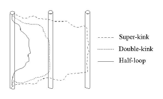
Figure 1: Thermally activated half-loop, double-kink, and super-kink excitations.

3.3 Static structure factor

The static structure factor, which is related to the scattering cross section, reveals spatial symmetries and ordered structures of materials in and out of equilibrium. It is basically the Fourier transform of the vortex density-density correlation function (here, in $d=2$ dimensions)

$$I(\boldsymbol{q})=\int\rme^{-\rmi\boldsymbol{q}\cdot(\boldsymbol{r}_{1}-\boldsymbol{r}_{2})}\,\langle n(\boldsymbol{r}_{1})\,n(\boldsymbol{r}_{2})\rangle\,\rmd^{\rmd}r_{1}\,\rmd^{\rmd}r_{2}=\langle n(\boldsymbol{q})\,n(\boldsymbol{-q})\rangle\ ,$$ (5)

where

$$n(\boldsymbol{q})=\int\rme^{-\rmi\boldsymbol{q}\cdot\boldsymbol{r}}\,n(\boldsymbol{r})\,\rmd^{\rmd}r$$ (6)

is the Fourier transform of the local vortex density $n(\boldsymbol{r})$. An ordered or quasi-ordered vortex structure such as the Abrikosov vortex lattice or Bragg glass would yield a periodic pattern of sharp peaks in the static structure factor. On the other hand, a disordered structure such as the vortex glass or vortex liquid would result in only a single diffuse peak at $\boldsymbol{q}=0$.

3.4 Voltage noise spectrum

The effect of disorder on the dynamics of driven vortices can also been studied by means of the velocity or voltage noise power spectrum which is defined by

$$S(\omega)=\Bigg{|}\int\boldsymbol{v}(t)\,\rme^{\rmi\omega t}\,\rmd t\Bigg{|}^{2}\ ,$$ (7)

and directly reflects periodicity of the average velocity in a moving vortex lattice. The voltage noise spectrum can display broadband or narrowband noise. It has been shown that in the presence of weak point defects, and at low driving force, vortices are in a plastic flow regime, characterized by a broadband noise signal $S(\omega)\sim\omega^{-\alpha}$ [44]. This power law may be interpreted as a remnant of the zero-temperature continuous depinning transition.

Narrowband noise is expected to exist provided the moving vortices maintain a long-range or quasi long-range positional order as in the moving Abrikosov vortex lattice or moving Bragg glass. For weak point or columnar pinning centers, a thorough study of the voltage noise power spectrum was reported in Ref. [30]. There, narrowband noise emerged at the characteristic washboard frequency which is given by $\omega=2\pi\langle v\rangle/a$, with the average velocity $\langle v\rangle$, and the typical intervortex distance $a$. The reason for the existence of this washboard noise is that quenched disorder in the system occasionally traps the vortices. As a consequence of the periodic vortex structure, this results in a periodically varying average overall velocity of the moving Abrikosov lattice or Bragg glass.

The existence of broadband noise and appearance of the washboard frequency in narrowband noise has been experimentally demonstrated [45]-[48] and numerically investigated both in two-dimensional [49]-[51] and three-dimensional systems [30, 33]. The magnitude of the broadband noise strongly depends on the applied current and the external field [52]. It was shown that the broadband noise in the ‘peak effect’ regime appears with the onset of vortex motion. The noise power increases to its maximum slightly above the critical current, and then decreases at large applied currents where the noise becomes suppressed. It was also suggested that the magnitude of the broadband noise would reach its maximum in the regime of plastic flow, and in three-dimensional simulations, narrowband noise with washboard frequency peaks was reported in the moving Bragg glass in the presence of weak pinning disorder [30]. In a recent experiment, narrowband noise was detected even in the peak effect regime, indicating apparent long-range temporal correlations of vortices near the critical temperature $T_{c}$ [53]. The characteristic frequency found in this experiment did not coincide with the washboard frequency, however: the associated length scale matched the sample width rather than the intervortex distance. Voltage noise has also been used to study the transition from a moving disordered phase, such as the moving vortex glass, to a moving ordered phase, such as moving Bragg glass or moving Abrikosov vortex lattice [33, 49]. The existence of washboard noise in systems with strong point or columnar defects is one of the issues to be addressed in this present study.

4 Simulation results

4.1 I-V characteristics

We first address the effect of different defect configuration on the I-V curves. In our simulations, we have studied six defect configurations: regular triangular and rectangular arrays of columnar defects; randomly placed splayed columnar defects; a mixture of point and randomly placed columnar defects; and randomly placed point defects. In order to generate columnar pinning centers, defect elements in each layer are arranged on top of each other which results in highly correlated defects with the highest critical currents. For our system with mixed point and linear defects, we chose the ratio between point and randomly placed columnar defect elements as 1:1. Splayed defects are created by placing columnar defects at random positions and tilting them slightly at fixed angle in random directions. In our simulations we tilt them such that the displacement between the top and the bottom layer for each defect is about 5 $b_{0}$. (A larger lateral displacement value would result essentially in a randomly placed point defect configuration and therefore lower critical currents.) With the same defect density, the difference in the value of critical currents for each I-V curve directly reflects the distinct spatial defect configurations. Small sample slices for each defect configuration type are depicted in figure 2.

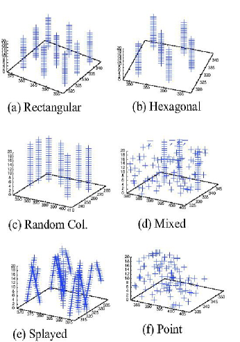
Figure 2: Small sample cross sections of systems with (a) rectangularly, (b) hexagonally, and (c) randomly placed columnar defects, (d) a mixed system with both randomly placed point and columnar pinning centers, and systems with (e) randomly placed splayed linear pins, and (f) point defects.

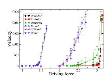
Figure 3: Force-velocity or I-V curves for systems with different defect configurations. Each system contains 16 flux lines. The systems with rectangularly (circles) and triangularly (squares) arranged columnar defects have higher critical currents than samples with randomly placed columnar defects (diamonds), splayed columnar defects (left triangles), a mixture between points and columnar defects (up triangle), or point defects (down triangle), respectively. This confirms that systems with correlated defects yield higher critical currents. Note that here the pinning strength (per unit length) for different defect configuration is set to be the same, 0.78 $\epsilon_{0}b_{0}$, while the real pinning strength for point defects is smaller by approximately an order of magnitude. Each of the data points was obtained from taking an average over 50 different defect realizations. Driving forces are given in units of $\epsilon_{0}/b_{0}$, and vortex velocities are measured in units $b_{0}$ / MCS.

Characteristic I-V curves for systems with different types of defect distributions are shown in figure 3. It is apparent that the critical currents for systems with triangular and rectangular arrangement of columnar defects are considerably higher than in samples with randomly placed columnar pins, randomly placed splayed columnar defects, a mixture of point and randomly placed columnar pinning centers, and randomly placed point defects, respectively. This is in good agreement with the experimental and numerical work [1, 24, 30], which clearly demonstrate that columnar defects are more effective and thus yield a larger critical current density $J_{c}$ than point pins. At low and intermediate drive, flux lines are trapped in metastable states and spend most of their time inside or in the immediate vicinity of the pinning potential. Flux line wandering between nearby defects may occur due to the thermally activated jumps. The average velocity is extremely small and can be explained by the theory of flux creep [54]. Far above the critical current, the flux lines flow freely. In the case of a system with randomly placed point defects, the pinning force density does not add coherently over the length of the vortex. Instead, the flux lines will attempt to find energetically optimized paths through the point pinning landscape, which promotes flux line wandering in the sample. Note that the real pinning strength for a columnar defect is stronger than for a point defect by approximately an order of magnitude. In our simulations, the pinning strength (per unit length) of all defect configurations is set to be the same, comparable to typical columnar pin strengths, whereas in Ref. [30] a much weaker pinning potential was chosen, more in line with typical oxygen vacancy pinning strengths. We have also confirmed that the depinning current (critical current at $T=0$) is lowered for all types of defects in denser vortex systems, where the repulsive vortex interactions tend to dominate over the attractive pinning energies [30, 31, 32]. This is demonstrated in figuress 4 and 5 for randomly placed columnar and point defects, respectively, showing the I-V characteristics obtained for systems with 16, 36, 64, and 100 lines in either case. In figure 6, we compare the approximate depinning forces or critical currents for systems with varying flux densities and randomly arranged columnar or point pinning centers, as obtained from the data shown in figures 4 and 5.

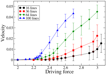
Figure 4: Force-velocity or I-V curves for systems with 1710 randomly placed columnar defects and different flux densities: 16 lines (circle), 36 lines (square), 64 lines (diamond), and 100 lines (triangle up). The depinning force or critical current becomes smaller for denser vortex systems.

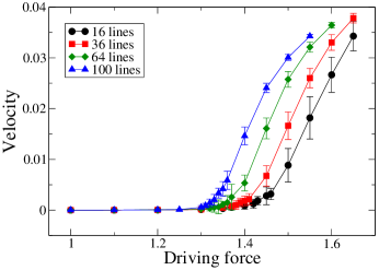
Figure 5: Force-velocity or I-V curves for systems with 34200 randomly placed point pinning centers and different flux densities: 16 lines (circle), 36 lines (square), 64 lines (diamond), and 100 lines (triangle up). Again, the depinning force or critical current goes down with increasing vortex density.

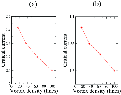
Figure 6: Critical current or depinning forces for (a) systems with randomly arranged columnar pins and (b) point defects as function of vortex density, as obtained from the data shown in figures 4 and 5.

4.2 Radius of gyration

Next we determined the root mean-square displacement or radius of gyration (4) near the depinning current, which allows us to obtain additional information about the shape of the moving flux lines in our three-dimensional samples. (This quantity is obviously not available in a two-dimensional simulation.) The radius of gyration represents the spatial fluctuations of the flux line from its center of mass. We omitted results in the regime of low driving forces since the dynamics there is extremely slow. Data in the regime of large driving forces are discarded also due to the unphysical limitation for each line element displacement as mentioned in the previous section.

4.2.1 Columnar defects.

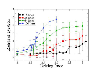
Figure 7: Mean radius of gyration (in units of $b_{0}$) along the drive direction for systems with randomly placed columnar defects with different flux densities: 16 lines (circle), 36 lines (square), 64 lines (diamond), and 100 lines (triangle up). The radius of gyration tends to grow at all drives as the density of flux lines increases, but saturates for dense systems. Recall that the mean columnar defect separation is 9 $b_{0}$.

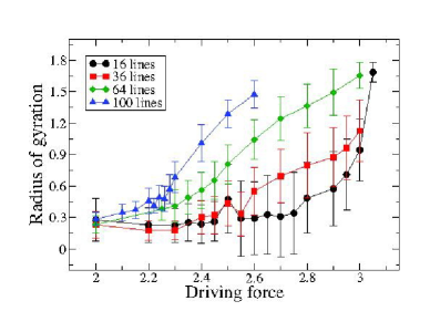
Figure 8: Mean radius of gyration in the direction transverse to the drive for systems with randomly placed columnar defects for different flux densities: 16 lines (circle), 36 lines (square), 64 lines (diamond), and 100 lines (triangle up).

Figures 7 and 8 display our results for the average radius of gyration (4) as functions of the driving force in systems of 16, 36, 64, and 100 flux lines with 1710 randomly placed columnar defects. For all investigated vortex densities, the radius of gyration in the direction of the drive increases with the driving force in the range studied here. At low drives, we observe the Bose glass phase with completely localized vortex lines inside the columnar defects as shown in the snapshot in figure 9a. In this state, the mean radius of gyration would be smaller than the columnar pin radius, which is set to 1 in our simulations. Since the pinning force of a columnar defect is very large and overcomes the repulsive vortex interaction, the flux lines become localized at different defect locations resulting in the disordered Bose glass phase. At intermediate drives close to the critical regime, some flux lines become delocalized and move along the drive direction, with enhanced transverse line fluctuations. This coexistence of a fluid of moving flux lines and the localized Bose glass is shown in figure 9b. One would expect a small average radius of gyration induced by the moving flux lines. At high drives, all flux lines are in motion, and hence a larger radius of gyration ensues, see figure 9c. The radius of gyration also increases with the number of vortices, but saturates at large flux densities, in our system at 64 and 100 lines, as shown in figure 7. This increase with flux density is again a consequence of the repulsive vortex interactions beginning to dominate over the attractive pinning energies. Flux lines are increasingly caged by their neighbors, and transverse wandering away from the linear defects becomes a collective excitation affecting several vortices. The observed saturation indicates that caging due to the effectively stronger vortex interaction at large densities governs the flux line dynamics at high driving currents. Notice that for the largest flux density in our simulation, the gyration radius reaches beyond the mean columnar pin distance, allowing for pinning of single lines to several defects. Qualitatively similar behavior of the mean radius of gyration is seen both along and transverse to the drive direction; vortex line fluctuations along the drive direction are however an order magnitude larger than the transverse fluctuations.

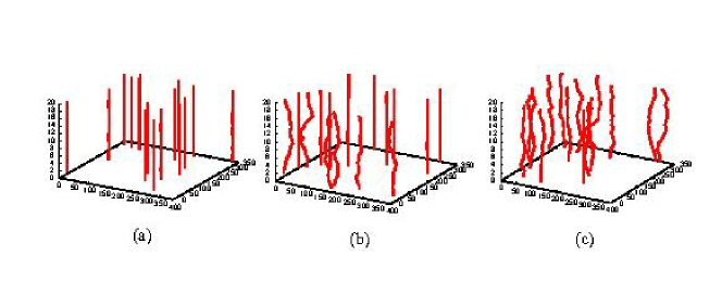
Figure 9: Snapshots of (moving) vortices in the presence of randomly placed columnar defects at (a) low, (b) intermediate, and (c) large drive. The flux line system is in the (a) pinned Bose glass phase, (b) partially pinned Bose glass and moving vortex glass / liquid phase, and (c) moving vortex glass / liquid phase.

Note that the above results differ characteristically from the data reported in Ref. [30] for systems with much smaller pinning strengths. In the moving vortex states of the weak pinning regime, the radius of gyration, both along the drive and transverse to it, was found to decrease for increasing flux density. This situation corresponds to a dynamics which is dominated by the vortex interaction rather than the pinning energies. This marked difference to the trend reported for our presented data arises from the fact that the pinning strength used in the current simulations is stronger by a factor of approximately 10: here we address a defect-dominated regime. In addition, we simulated our system with a larger penetration length which requires a larger system size in order to avoid the numerical artifact due to the interaction cut-off. With the same number of vortex lines, but in a larger system size and much stronger pinning strength, we are here working in a regime where the flux lines are rather weakly interacting, and their structure and dynamics is dominated by the defects. Thus, the investigated current range effectively remains rather close to the depinning threshold.

4.2.2 Point defects.

Point defects directly affect the vortex dynamics. In contrast to systems with columnar defects, uncorrelated point disorder promotes spatial wandering, transverse to the magnetic field direction, of the moving flux lines. The spatially randomly distributed pinning centers try to pull the vortex lines in different directions as they traverse the sample, which leads to less effective pinning compared to linear defects. In the regime where the defects dominate the dynamics, the radius of gyration for point defect is then expected to be larger than for systems with columnar pins.

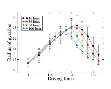
Figure 10: Mean radius of gyration along the drive direction for systems with point defects with different flux densities: 16 lines (circle), 36 lines (square), 64 lines (diamond), and 100 lines (triangle up). The radius of gyration starts to grow as the drive increases, reaching its highest value at the critical current; at larger drives, it decreases again. Note that even for the largest flux density the peak gyration radius is only about 1/2 the corresponding vortex lattice constant, see table 1.

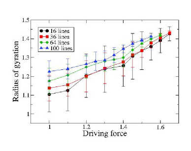
Figure 11: Mean radius of gyration transverse to the drive and magnetic field for systems with point defects with different flux densities: 16 lines (circle), 36 lines (square), 64 lines (diamond), and 100 lines (triangle up). The radius of gyration grows monotonously as the drive increases.

Figure 10 shows the radius of gyration along the direction of the drive. The shape of the curve differs from the one depicted in figure 7 for randomly placed columnar defects. At small drives, the radius of gyration at a specific driving force slightly increases with growing flux density, while we observed a larger deviation in the system with columnar defects. For increasing drives, the radius of gyration keeps growing and reaches its maximal value just above the depinning threshold. This indicates that the dynamics of the system is only marginally dominated by the point pinning centers, and only until the critical threshold is reached. In an infinite system at zero temperature, critical fluctuations would lead to a divergence of the mean radius of gyration at the nonequilibrium depinning phase transition. In the moving glass phase, we observe that the gyration radius decreases with flux density. At lower densities, point disorder plays a more prominent role, and has the effect of enhancing flux wandering which allows the vortex lines to more efficiently explore favorable sites in the pinning landscape. We note that the gyration radius along the drive direction peaks at values well below the typical vortex lattice constants, see table 1.

The radius of gyration in the direction transverse to the drive behaves quite differently. As shown in figure 11, at any vortex density the transverse radius of gyration keeps monotonously increasing with the driving force, and no tendency of a maximum or saturation is evident. The curves tend to merge towards the same value at high drive. The transverse radius of gyration is hardly affected by the drive; flux lines can only diffuse about their center of mass in the absence of the drive. The distance that the flux line element can move away from the center of mass is limited by the elastic line tension, which tries to pull the vortex line element back towards its center of mass. For increasing vortex density, the radius of gyration becomes larger since the dynamics becomes increasingly dominated by the vortex interactions rather than the pinning potentials; displacement of a line element of any vortex thus typically induces motion of nearby elements of other flux lines as well. Snapshots of moving vortices subject to point pinning centers at different drives are plotted in figure 12; Figure 12b at intermediate driving force corresponds to the largest radius of gyration observed in our simulations. Indeed, transverse line wandering is prominent near the depinning current, as is evident in figure 12b. (Note, however, that the layer-to-layer displacements still range within the applicability limit of the London approximation.)

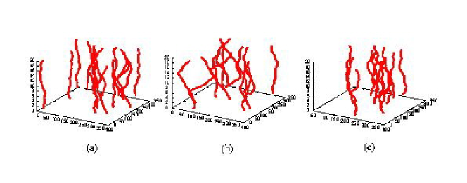
Figure 12: Snapshots of moving vortices in the presence of randomly placed point defects at (a) low, (b) intermediate, and (c) large drive. Flux lines are in the (a) pinned vortex glass phase, (b) and (c) moving liquid / vortex glass phase. The vortices display the largest average radius of gyration at intermediate drive.

4.3 Half-loop and double-kink excitations

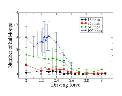
Figure 13: Measured number of half-loops for systems with random columnar defects with different flux densities: 16 lines (circle), 36 lines (square), 64 lines (diamond), and 100 lines (triangle up). The number of half-loops shows a maximum just above the critical current and then tends to decrease at all drives as the density of flux lines increases.

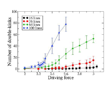
Figure 14: Measured number of double-kinks for systems with random columnar defects with different flux densities: 16 lines (circle), 36 lines (square), 64 lines (diamond), and 100 lines (triangle up). The number of double-kinks tends to increase with growing vortex density at all drives, similar to the mean radius of gyration.

The crossover of the dynamics from a disorder- to an interaction-dominated regime as induced by the driving force has been explained in the previous section. A large mean vortex radius of gyration appears at elevated driving forces for systems with both randomly placed point and columnar defects. At low driving force, the structure of the flux line system is different in both cases. Columnar defects tend to straighten the flux lines, whereas in a system with point defects flux line wandering is promoted. At low driving force, we observed the localized Bose glass in systems with columnar defects. At low temperatures and low external driving current, flux creep happens via the formation of vortex half-loop, double-kink, and superkink excitations (see figure 1) [19, 55, 56], which represent saddle point configurations whose excitation energies $U_{\rm b}(J)$ represents the effective current-depending barrier energy that enters the thermal activation factor $\exp[-U_{\rm b}(J)/T]$ for flux flow. In the localized Bose glass phase, these excitations occurred extremely rarely in our simulations, preventing us from obtaining statistically significant data.

At intermediate driving forces near the depinning threshold, however, half-loop excitations become quite prominent, as seen in figure 13, and at given vortex density, their typical number decreases with increasing drive. Also, a larger number of half-loop excitations is observed as the density is increased, which indicates again that the vortex interactions play an important role for the existence of multiple, ‘coherent’ half-loop excitations.

We do not observe double kinks at small driving currents; they only appear at drives larger than the critical depinning force. The presence of double-kinks is largely due to an interplay of pulling on the vortices and strong pinning forces rather than thermal fluctuations. As a flux line is moving, some vortex elements will enter columnar pinning centers. These flux line elements become trapped while other segments are pulled along the drive direction. The vortex line keeps stretching until the elastic energy overcomes the pinning energy, whereupon the trapped flux line elements depin from the defect. This would result in the emergence of double-kinks, as depicted in figure 14. These prominent double-kinks are likely largely responsible for the observed continuing increase of the mean radius of gyration, see figure 7.

4.4 Static structure factor

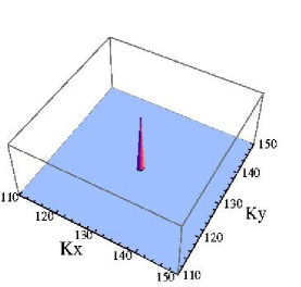
Figure 15: Static structure factor plot of moving vortex lines in a system with randomly placed point defects in the nonequilibrium steady state. The strong pinning centers destroy any translational order, and the ensuing single structure factor peak indicates a moving plastic or liquid phases of vortices, as also seen in the snapshot 12c. We obtain similar static structure factors at all vortex densities, driving forces, and for all defect configurations studied here.

In this present study, the abundant point or linear pinning centers are always sufficiently strong to destroy any spatially ordered structures in the accessible range of driving forces. In contrast with our earlier investigations of vortex transport in the presence of much weaker pinning sites [30], here we observe neither positional nor orientational long-range order. In this strong pinning situation, flux transport happens via plastic or liquid motion at drives larger than the depinning force. Correspondingly, we observe a single peak in the static structure factor of the moving vortex system, for all defect configurations investigated here. This corresponds to a single peak in the diffraction plot as the experimental signature for plastic motion [32, 57]. As an example, figure 15 shows the structure factor (5) obtained from our simulations for a system with point defects. The single peak indicates the presence of an isotropic liquid or a disordered solid of moving flux lines, as indeed confirmed by the snapshot depicted in figure 12c. (We have also measured the static structure factor in a different system with weak pinning defects, and instead observed hexagonal Bragg peaks corresponding to the triangular moving vortex lattice or Bragg glass.)

4.5 Voltage noise spectrum

Finally, we report and discuss the measured voltage noise power spectrum (7) stemming from the vortex motion in systems with randomly placed point and columnar defects.

4.5.1 Randomly placed point defects.

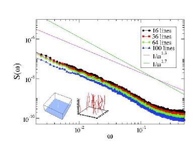
Figure 16: Voltage noise along the drive direction for systems with randomly placed point defects at various vortex densities. The driving force along the x-axis for each curve was set to 1.5. The noise amplitude grows as the vortex density increases from 16 to 36, 64, and 100 lines in the system. The broadband noise in these systems reflects the presence of a moving disordered phase, such as a moving liquid or plastic phase. This is also supported by the structure factor plot and the snapshot shown in the inset. The power laws $S(\omega)\propto 1/\omega^{1.3}$ and $S(\omega)\propto 1/\omega^{1.7}$ are indicated also, to match to the data at low and intermediate frequencies, respectively.

As shown in figure 16, we observe broadband noise in our simulations of systems with point defects at all vortex densities. The results are averaged over 50 defect realizations and initial vortex positions. We specifically investigate the regime where the driving force is set to 1.5, and after the system has reached its nonequilibrium steady state. The absence of narrowband noise indicates the presence of a moving vortex liquid phase, in agreement with experiments in the peak effect regime [52]. This interpretation is supported by the appearance of the single peak in the structure factor and the snapshot of the moving vortices in the inset of figure 16. Each flux line in this system subject to strong point disorder moves largely independently, which implies the loss of any washboard signal in contrast with the results obtained in samples with very weak point defects [30]. In the presence of weak pinning centers, the vortices arrange themselves into the quasi long-range ordered moving Bragg glass, and essentially move with the same speed. As this ordered structure traverses the disordered substrate with almost homogeneous speed $\langle v\rangle$, periodic trapping induces a narrowband washboard noise signal with a characteristic peak frequency $\omega=2\pi\langle v\rangle/a_{0}$, where $a_{0}$ denotes the vortex lattice constant.

The magnitude of the broadband noise signal decreases for increasing vortex density, indicating that the flux lines tend to reorder at higher flux density. This is also reflected by the decrease of the radius of gyration for increasing vortex density. The magnitude of the noise indicates the fluctuations of the velocity about its mean. At higher flux densities, the vortex interactions dominate and cause a stiffening of the flux lines as they become caged by their neighbors. Stronger vortex interactions favor the Abrikosov vortex lattice or Bragg glass with reduced noise. A decrease of the noise power for increasing vortex density or interaction strength has also been reported in experimental data [52] and numerical simulations [49].

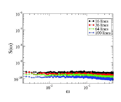
Figure 17: Voltage noise in the transverse direction to the driving force (y-direction) for systems with randomly placed point defects at various vortex densities. The driving force along the x-axis for each curve is set to 1.5. Similar to the voltage noise in the x-direction, the magnitude for each curve decreases as the vortex density increases from 16 to 36, 64, and 100. The broadband noises in these systems reflect the property of a moving disordered phase.

A power law broadband noise spectrum $S(\omega)\sim 1/\omega^{\alpha}$ was also reported in simulations of two- and three-dimensional XY and dual Coulomb gas models [44], where at zero magnetic field an exponent $\alpha=1.5$ was found, whereas $\alpha\approx 1$ in a system with small applied magnetic field. These results are similar to the experimental data reported in Refs. [58, 59], where the voltage noise spectrum decays at high frequency like $1/\omega$ at elevated temperature and like $1/\omega^{3/2}$ at lower temperature. The exponent $\alpha=1.5$ also emerges from a functional renormalization group calculation for point defects to one-loop order in three dimensions [60]. The voltage noise power spectrum in our data, with strong pinning centers, varies approximately like $S(\omega)\sim 1/\omega^{\alpha}$ with $\alpha\approx 1.3$, which is well fitted in the low frequency regime, whereas we find $\alpha\approx 1.7$ at intermediate frequencies. Our exponent value is smaller than the exponent $\alpha=2$, which is in fact the mean-field value, and was measured in a system of non-interacting driven vortices subject to weak point and columnar defects [40].

As shown in figure 17, the y-component of the broadband noise is observed to be nearly flat white noise, and to decrease in magnitude for increasing vortex density. Transverse to the drive direction, there are much smaller velocity fluctuations, and no typical time scale exists. Each moving flux line can only fluctuate around its center of mass which results in zero average velocity.

4.5.2 Randomly placed columnar defects.

In our system with 1710 randomly placed parallel columnar defects, we observe narrowband voltage noise peaks on top of a broadband background, as shown in figure 18 for systems with a 16, 36, 64, and 100 flux lines, with the data taken in the nonequilibrium steady state at driving force 2.7 along the x direction, and the average taken over 50 realizations of the defect and initial vortex positions. As can be readily confirmed by computing the associated characteristic time, the presence of these narrowband peaks at low frequencies can however be simply attributed to the traversal time of the vortices through the entire system. The observed periodicity is merely due to the moving vortices encountering the identical linear defect configurations in our system with periodic boundary conditions. Even though our system with point defects has similarly strong pinning centers, no narrowband peaks are observed here since each flux line element moves almost independently. During their repeated traversal through the sample, each flux line element may become trapped at point pins at different locations. The various associated time scales yield quite different frequencies and result in the characteristic broadband noise. In comparison to the system with point defects, our sample with randomly placed columnar pins yields a power law $S(\omega)\sim 1/\omega$ in the low frequency regime. Thus, different defect configurations induce distinct values of the broadband noise scaling exponent: correlated defects produce a larger exponent value in the strong pinning regime.

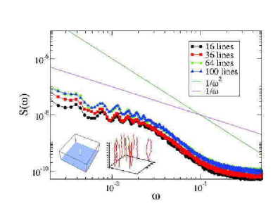
Figure 18: Voltage noise power spectrum in the direction of the driving force for systems with randomly placed columnar defects at various flux densities. The driving force along the x axis for each curve is set to 2.7. The amplitude for each curve increases with the vortex density. The low-frequency oscillations originate from repeated traversal through the finite system with periodic boundary conditions.

5 Discussion and conclusion

In this paper, we have presented numerical investigations of the nonequilibrium steady states of driven magnetic flux lines in type-II superconductors subject to various configurations of strong point or columnar pinning centers. We have employed a versatile three-dimensional Metropolis Monte Carlo code based on an elastic line model and used the measured current-voltage curve, vortex structure factor, mean radius of gyration, number of half-loop and double-kink excitations, and the voltage noise power spectrum to thoroughly characterize the ensuing moving vortex structures and fluctuations.

Interesting features arise due to the competition between the elastic energy, pinning potential, repulsive vortex interactions, and the driving force. In the absence of the driving force and defects, we observed the Abrikosov vortex lattice as expected. A pinned vortex glass is found in systems with strong point defects, while a localized Bose glass is observed in the presence of strong columnar defects. From our simulation results, the snapshots of these two systems from the top view look very similar, i.e., each flux line looks like a point-like particle located inside the pinning center. However, these flux line systems behave quite differently if a small driving force is applied. The effect due to different defect structures is reflected in their different force-velocity or I-V curves. We have found that systems with correlated defects such as parallel or splayed columnar defects yield higher critical depinning currents. The presence of strong point defects strongly promotes flux line wandering, which results in a liquid-like vortex structure. This feature is also captured by measuring the radius of gyration and studying snapshots of the driven vortex system. By investigating the radius of gyration for various driving forces, we observed that the driving force changed the moving flux line dynamics from a regime dominated by the disorder at low drives to a regime dominated by the vortex interactions at high drives. This is, for example, evident in the system with point defects as the driving force or the vortex density are varied. In contrast, in systems with weak pinning centers the disorder-dominated regime is not accessible.

In the low driving force regime, we did not observe double-kinks excitations, but a small number of half-loop excitations were detectable at intermediate driving forces. At large driving force, we observed a liquid-like or amorphous disordered structure of moving flux lines in our samples with strong point or columnar defects. The static structure factor in all our results show a single peak which corresponds to a disordered structure. Another noticeable difference between the vortex systems subject to point and columnar pinning centers emerges when studying the voltage noise spectrum. While just above the critical threshold broadband noise is observed at all vortex densities and driving forces in either case, the characteristic exponent describing the power-law decay of the voltage noise signal turns out to be larger for randomly distributed point defects.

References

References

- [1] Blatter G, Feigel’man M V, Geshkenbein V B, Larkin A I and Vinokur V M 1994 Rev. Mod. Phys. 66, 1125.
- [2] Bolle C A, De La Cruz F, Gammel P L , Waszczak J V and Bishop D J 1993 Phys. Rev. Lett. 71, 4039.
- [3] Chang A M et al1992 Appl. Phys. Lett. 61, 1974.
- [4] Gammel P L et al1994 Phys. Rev. Lett. 72, 278.
- [5] Hess H F, Murray C A and Waszczak J V 1992 Phys. Rev. Lett. 69, 2138.
- [6] Harada K et al1993 Phys. Rev. Lett. 71, 3371.
- [7] Yaron U et al1994 Phys. Rev. Lett. 73, 2748.
- [8] Nattermann T 1990 Phys. Rev. Lett. 64, 2454.
- [9] Giamarchi T and Le Doussal P 1994 Phys. Rev. Lett. 72, 1530.
- [10] Giamarchi T and Le Doussal P 1995 Phys. Rev. B 52, 1242.
- [11] Kierfeld J, Nattermann T and Hwa T 1997 Phys. Rev. B 55, 626.
- [12] Fisher D S 1997 Phys. Rev. Lett. 78, 1964.
- [13] Le Doussal P and Giamarchi T 1997 Phys. Rev. B 55, 6577.
- [14] Giamarchi T and Le Doussal P 1996 Phys. Rev. Lett. 76, 3408.
- [15] Fisher M P A 1989 Phys. Rev. Lett. 62, 1415.
- [16] Feigel’man M V, Geshkenbein V B, Larkin A I and Vinokur V M 1989 Phys. Rev. Lett. 63, 2303.
- [17] Nattermann T 1990 Phys. Rev. Lett. 64, 2454.
- [18] Fisher D S, Fisher M P A and Huse D A 1990 Phys. Rev. B 43, 130.
- [19] Nelson D R and Vinokur V M 1992 Phys. Rev. Lett. 68, 2398.
- [20] Lyuksyutov I F 1992 Europhys. Lett. 200, 273.
- [21] Nelson D R and Vinokur V M 1993 Phys. Rev. B 48, 13060.
- [22] Fisher M P A, Weichman P B, Grinstein G and Fisher D S 1989 Phys. Rev. B 40, 546.
- [23] Täuber U C and Nelson D R 1997 Phys. Rep. 289 157.
- [24] Civale L et al1991 Phys. Rev. Lett. 67, 648.
- [25] Kardar M 1998 Phys. Rep. 301, 85.
- [26] Fisher D S 1998 Phys. Rep. 301, 113.
- [27] Le Doussal P and Giamarchi T 1996 Phys. Rev. Lett. 76, 3408.
- [28] Le Doussal P and Giamarchi T 1998 Phys. Rev. B 57, 11356.
- [29] Olive E, Soret J C, Le Doussal P and Giamarchi T 2003 Phys. Rev. Lett. 91, 037005.
- [30] Bullard T J, Das J, Daquila G L and Täuber U C 2008 Eur. Phys. J. B 65, 469.
- [31] Olson C J, Zimanyi G T, Kolton A B and Gronbach-Jensen N 2000 Phys. Rev. Lett. 85, 5416.
- [32] Kolton A B, Dominguez D, Olson C J and Gronbach-Jensen N 2000 Phys. Rev. B 62, R14657.
- [33] Chen Q and Hu X 2003 Phys. Rev. Lett. 90, 117005.
- [34] Chen Q and Hu X 2007 Phys. Rev. B 75, 064504.
- [35] Dong M, Marchetti M C and Middleton A A 1993 Phys. Rev. Lett. 70, 662.
- [36] Tang C, Feng S and Golubovic L 1994 Phys. Rev. Lett. 72, 1264.
- [37] Sen P, Trivedi N and Ceperley D M 2001 Phys. Rev. Lett. 86, 4092.
- [38] Rosso A and Krauth W 2001 Phys. Rev. B 65, 012202.
- [39] Tyagi S and Goldschmidt Y Y 2003 Phys. Rev. B 67, 214501.
- [40] Das J, Bullard T J and Täuber U C 2003 Physica A 318, 48.
- [41] Bullard T J, Das J and Täuber U C 2004 Trends in Superconductivity Research p 63.
- [42] Petäjä V, Alava M and Rieger M 2004 Europhys. Lett. 66, 778.
- [43] Lawrence W E and Doniach S 1970 and 1971 Proc. 12th Int. Conf. Low Temp. Phys. ed Kanda E (Kyoto, Keigaku Tokyo) p 361.
- [44] Vestergren A and Wallin M 2004 Phys. Rev. B 69, 144522.
- [45] Fiory A T 1971 Phys. Rev. Lett. 27, 501.
- [46] Harris J M, Ong N P, Gagnon R and Taillefer L 1995 Phys. Rev. Lett. 74, 3684.
- [47] Troyanovski A M, Aarts J and Kes P H 1999 Nature (London) 399, 665.
- [48] Togawa Y, Abiru R, Iwaya K, Kitano H and Maeda A 2000 Phys. Rev. Lett. 85, 3716.
- [49] Olson C J, Reichhardt C and Nori F 1998 Phys. Rev. Lett. 81, 3757.
- [50] Kolton A B, Dominguez D and Gronbech-Jensen N 2002 Phys. Rev. B 65, 184508.
- [51] Fangohr H, Cox S J and de Groot P A J 2001 Phys. Rev. B 64, 064505.
- [52] Marley A C et al1995 Phys. Rev. Lett. 74, 3029.
- [53] Pautrat A and Scola J 2009 Phys. Rev. B 79, 024507.
- [54] Anderson P W 1962 Phys. Rev. Lett. 9, 309.
- [55] Hwa T, Nelson D R and Vinokur V M 1993 Phys. Rev. B 48, 1167.
- [56] Täuber U C, Dai H, Nelson D R and Lieber C M 1995 Phys. Rev. Lett. 74, 5132.
- [57] Kolton A B and Dominguez D 1999 Phys. Rev. Lett. 83, 3061.
- [58] Rogers C T, Myers K E, Eckstein J N and Bozovic I 1992 Phys. Rev. Lett. 69, 160.
- [59] Festin Ö, Svedlindh P, Kim B J, Minnhagen P, Chakalov R and Ivanov Z 1999 Phys. Rev. Lett. 83, 5567.
- [60] Ertas D and Kardar M 1994 Phys. Rev. Lett. 73, 1703.