Sequential optimizing strategy in multi-dimensional bounded forecasting games

Abstract

We propose a sequential optimizing betting strategy in the multi-dimensional bounded forecasting game in the framework of game-theoretic probability of Shafer and Vovk (2001). By studying the asymptotic behavior of its capital process, we prove a generalization of the strong law of large numbers, where the convergence rate of the sample mean vector depends on the growth rate of the quadratic variation process. The growth rate of the quadratic variation process may be slower than the number of rounds or may even be zero. We also introduce an information criterion for selecting efficient betting items. These results are then applied to multiple asset trading strategies in discrete-time and continuous-time games. In the case of continuous-time game we present a measure of the jaggedness of a vector-valued continuous process. Our results are examined by several numerical examples.

Keywords and phrases: game-theoretic probability, Hölder exponent, information criterion, Kullback-Leibler divergence, quadratic variation, strong law of large numbers, universal portfolio.

1 Introduction

Since the advent of the game-theoretic probability and finance by Shafer and Vovk [10], the field has been expanding rapidly. The present authors have been contributing to this emerging field by showing the essential role of the Kullback-Leibler divergence for the strong law of large numbers (SLLN) [8, 9] and by proposing a new approach to continuous-time games [12, 13]. Our approach to continuous-time games has been further developed by V. Vovk [14, 15, 16].

In this paper we propose a sequential optimizing betting strategy for the multi-dimensional bounded forecasting game in discrete time and apply it as a high-frequency limit order type betting strategy for vector-valued continuous price processes.

Our strategy is very flexible and the analysis of its asymptotic behavior allows us to generalize game-theoretic statements of SLLN to a wide variety of cases. SLLN for the bounded forecasting game is already established in Chapter 3 of [10]. In [8] we gave a simple strategy forcing SLLN with the rate of $O(\sqrt{\log n/n})$, where $n$ is the number of rounds. However the convergence rate of SLLN should depend on the growth rate of the quadratic variation process. For example, in view of Kolmogorov’s three series theorem (e.g. Section IV.2 of [11]), the sum $s_{n}=x_{1}+\dots+x_{n}\in{\mathbb{R}}^{1}$ of centered independent measure-theoretic random variables converges a.s. if the sum of their variances converges (i.e. $\sum_{n}{\rm Var}(x_{n})<\infty$). Therefore in this case the sample average $\bar{x}_{n}=s_{n}/n$ is of order $O(1/n)$. By our sequential optimizing betting strategy, we can give a unified game-theoretic treatment on the asymptotic behavior of $s_{n}$, which depends on the asymptotic behavior of $\sum_{i=1}^{n}x_{i}^{2}$ as $n\rightarrow\infty$.

The strength of our results can be seen when we interpret our results in the standard measure-theoretic framework. Let $s_{n}=x_{1}+\dots+x_{n}$ be a one-dimensional measure-theoretic martingale w.r.t. a filtration $\{{\cal F}_{n}\}$ with uniformly bounded differences $\|x_{n}\|\leq 1$, a.e. Let $V_{n}=x_{1}^{2}+\dots+x_{n}^{2}$. Then with probability one the sequence $\|s_{n}\|/\sqrt{\max(0,V_{n}\log V_{n})}$, $n=1,2,\dots$, is bounded. See Proposition 2.1 below. Note that in this statement no assumption is made on the growth rate of $V_{n}$. The rate itself may be random.

From more practical viewpoint, our sequential betting strategy is very simple to implement even for high dimensions and shows a very competitive performance when applied to various price processes. In Section 6 we compare the performance of our strategy with the well-known universal portfolio strategy developed by Thomas Cover and collaborators ([3, 4, 5, 6]). The performance of our sequential betting strategy is competitive against the universal portfolio. Note that the numerical integration needed for implementing universal portfolio is computationally heavy for high dimensions.

When we can bet on a large number of price processes, it is not always best to form a portfolio comprising all price processes, because estimating the best weight vector for the price processes might take a long time. By approximating the capital process of our sequential optimizing strategy, we will introduce an information criterion for selecting price processes in a portfolio.

The organization of this paper is as follows. In Section 2 we formulate the multi-dimensional bounded forecasting game, introduce our sequential optimizing strategy and state our main theoretical result. In Section 3 we give a proof of our result by analyzing asymptotic behavior of its capital process. We also introduce an information criterion for selecting efficient betting items. These results are then applied to multiple asset trading games in Section 4. In Section 4 we formulate the multiple asset trading game in continuous time and based on high-frequency limit order type betting strategies we present a measure for the jaggedness of a path of a vector-valued continuous process. In Section 5, as indicating the generality of our results, we provide a multiple type of Girsanov’s theorem for geometric Brownian motion and an argument concerning the mutual information quantity between betting games. In Section 6 we give numerical results for several Japanese stock price processes. We conclude the paper with some remarks in Section 7.

2 A sequential optimizing strategy and its implication to strong law of large numbers

We treat the following type of discrete time bounded forecasting game between Skeptic and Reality. ${\cal K}_{0}$ is the initial capital of Skeptic, $D$ is a compact region in ${\mathbb{R}}^{d}$ such that its convex hull $\mathop{{\rm co}}D$ contains the origin in its interior, and $\cdot$ denotes the standard inner product of ${\mathbb{R}}^{d}$.

Discrete Time Bounded Forecasting Game
Protocol:

${\cal K}_{0}:=1$.
FOR $n=1,2,\dots$:
Skeptic announces $M_{n}\in{\mathbb{R}}^{d}$.
Reality announces $x_{n}\in D$.
${\cal K}_{n}={\cal K}_{n-1}+M_{n}\cdot x_{n}$.
END FOR

In this paper we regard $d$-dimensional vectors such as $x_{n}=(x_{n}^{1},\dots,x_{n}^{d})^{\mathrm{t}}$ as column vectors with ^t denoting the transpose. $\|x\|=\sqrt{x^{\mathrm{t}}x}=\sqrt{x\cdot x}$ denotes the Euclidean norm of $x$. Letting $\alpha_{n}=M_{n}/{\cal K}_{n-1}$, we can rewrite Skeptic’s capital as ${\cal K}_{n}={\cal K}_{n-1}(1+\alpha_{n}\cdot x_{n}),\ \alpha_{n}\in{\mathbb{R}}^{d}$. In the protocol, we require that Skeptic observes his collateral duty, in the sense that ${\cal K}_{n}\geq 0$ for all $n$ irrespective of Reality’s moves $x_{1},x_{2},\dots$.

For constructing a strategy of Skeptic, consider that Skeptic himself generates ‘training data’ $\{x_{-n_{0}+1},x_{-n_{0}+2},\dots,x_{0}\}$ of size $n_{0}\geq d+1$. This operation is similar to a construction of a prior distribution in Bayesian statistics, where a prior distribution can be specified by a set of prior observations. Throughout this paper we fix an arbitrarily $\epsilon_{0}\in(0,1)$ and choose the training data $\{x_{-n_{0}+1},\dots,x_{0}\}$ in such a way that

$$1+\alpha\cdot x_{n}\geq 0,\ n=-n_{0}+1,\dots,0,\quad\Rightarrow\quad 1+\alpha\cdot x\geq\epsilon_{0},\ \forall x\in D.$$ (1)

Let $P^{d}_{n_{0},\epsilon_{0}}=\{\alpha\mid 1+\alpha\cdot x_{n}\geq 0,\ n=-n_{0}+1,\dots,0\}$. Then (1) is equivalent to

$$P^{d}_{n_{0},\epsilon_{0}}\subset-(1-\epsilon_{0})(\mathop{{\rm co}}D)^{\perp},$$

where $(\mathop{{\rm co}}D)^{\perp}$ denotes the convex dual of $\mathop{{\rm co}}D$. For example, for $d=1$ and $D=[-1,1]$, we can take $x_{-1}=1/(1-\epsilon_{0})$ and $x_{0}=-1/(1-\epsilon_{0})$. Then $\alpha$ has to satisfy $|\alpha|\leq 1-\epsilon_{0}$ and the right-hand side of (1) holds. For general $D\subset{\mathbb{R}}^{d}$ let $\bar{\delta}=\max_{x\in D}\|x\|$ and let $c=\bar{\delta}\sqrt{d}/(1-\epsilon_{0})$. Then we can take $n_{0}=2d$ training vectors as

$$(0,\dots,0,\pm c,0,\dots,0)^{\mathrm{t}},$$

where $c$ is in the $i$-th coordinate ($1\leq i\leq d$). Then each element $\alpha^{i}$, $1\leq i\leq d$, of $\alpha=(\alpha^{1},\dots,\alpha^{d})^{\mathrm{t}}$ has to satisfy $|\alpha^{i}|\leq 1/c$ and $\|\alpha\|\leq(1-\epsilon_{0})/\bar{\delta}$. Hence the right-hand side of (1) holds by Cauchy-Schwarz inequality. It should also be noted that (1) implies that the training vectors span the whole ${\mathbb{R}}^{d}$.

The strategy with a constant vector $\alpha_{n}\equiv\alpha\in{\mathbb{R}}^{d}$ is called a constant proportional betting strategy. For $N\geq 0$ we define

$$\Phi_{0,N}(\alpha)=\sum_{n=-n_{0}+1}^{N}\log(1+\alpha\cdot x_{n}),$$ (2)

which is the log capital at round $N$ under the constant proportional betting strategy, including the training data. We add ‘$0$’ to the subscript to indicate that the training data are included in a summation. Since the game starts at time $1$, actually the log capital of the constant proportional betting strategy is $\Phi_{0,N}(\alpha)-\Phi_{0,0}(\alpha)=\sum_{n=1}^{N}\log(1+\alpha\cdot x_{n})$.

Let us consider the maximization of $\Phi_{0,N}(\alpha)$ with respect to $\alpha\in{\mathbb{R}}^{d}$. The maximum corresponds to the log capital at time $N$ of a ‘hindsight’ constant proportional betting strategy. Note that $\Phi_{0,N}(\alpha)$ is a strictly concave function of $\alpha$. The condition (1) ensures that the maximum of $\Phi_{0,N}(\alpha)$ is attained at the unique point $\alpha=\alpha_{N}^{*}$ in the interior of $P^{d}_{n_{0},\epsilon_{0}}$ so that

$$\frac{\partial\Phi_{0,N}}{\partial\alpha}\Bigm{|}_{\alpha=\alpha_{N}^{*}}=\sum_{n=-n_{0}+1}^{N}\frac{x_{n}}{1+\alpha_{N}^{*}\cdot x_{n}}=0.$$ (3)

From numerical viewpoint we note that the numerical maximization of $\Phi_{0,N}(\alpha)$ is straightforward even in high dimensions.

We now define sequential optimizing strategy (SOS) of Skeptic, which is a realizable strategy unlike the hindsight strategy. It is given by

$$\alpha_{n}=\alpha_{n-1}^{*},\ \ n\geq 1.$$ (4)

The idea of SOS is very simple. We employ the empirically best constant proportion until the previous round for betting at the current round. Note that SOS depends on the choice of the training data. Skeptic’s log capital $\log{\cal K}_{1,N}^{*}$ at round $N$ under SOS is written as

$$\log{\cal K}_{1,N}^{*}=\sum_{n=1}^{N}\log(1+\alpha_{n-1}^{*}\cdot x_{n}).$$

Let $\xi=x_{1}x_{2}\dots\in D^{\infty}$ denote a path, which is an infinite sequence of Reality’s moves. The set $\Omega=D^{\infty}$ of paths is called the sample space and any subset $E$ of $\Omega$ is called an event. $\xi^{n}=x_{1}\dots x_{n}$ denotes a partial path of Reality until the round $n$. A strategy ${\cal P}$ specifies $\alpha_{n}$ in terms of $\xi^{n-1}$, i.e. $\alpha_{n}={\cal P}(\xi^{n-1})$. The capital process under ${\cal P}$ is given as ${\cal K}^{{\cal P}}_{1,N}=\prod_{n=1}^{N}(1+{\cal P}(\xi^{n-1})\cdot x_{n})$. ${\cal P}$ is called prudent, if Skeptic observes his collateral duty by ${\cal P}$, i.e.  ${\cal K}^{{\cal P}}_{1,N}\geq 0$, $\forall N\geq 0$, irrespective of Reality’s moves $x_{1},x_{2},\dots$. In this paper we only consider prudent strategies of Skeptic. We say that Skeptic can weakly force an event $E\subset\Omega$ by a strategy ${\cal P}$ if $\limsup_{N}{\cal K}^{{\cal P}}_{1,N}=\infty$ for every $\xi\not\in E$. As in Section 1 we write

$$s_{N}=x_{1}+\dots+x_{N}\in{\mathbb{R}}^{d},\quad V_{N}=x_{1}x_{1}^{\mathrm{t}}+\cdots+x_{N}x_{N}^{\mathrm{t}}\quad(:d\times d).$$ (5)

Then $\mathop{{\rm tr}}V_{N}=\sum_{n=1}^{N}\|x_{n}\|^{2}$. We are now ready to state our main theorem.

Theorem 2.1.

By the sequential optimizing strategy Skeptic can weakly force

$$E:\limsup_{N}\frac{\|s_{N}\|}{\sqrt{\max(1,\mathop{{\rm tr}}V_{N}\log(\mathop{{\rm tr}}V_{N})})}<\infty.$$ (6)

The maximum in the denominator is needed only for the case that $\sup_{N}\mathop{{\rm tr}}V_{N}\leq 1$, such as $0\in D$ and Reality always chooses $x_{n}\equiv 0$. It is important to emphasize that $E$ in (6) is weakly forced irrespective of the rate of growth of $\mathop{{\rm tr}}V_{N}$, including the zero-growth case, i.e. the case that $\mathop{{\rm tr}}V_{N}$ converges to a finite value. A measure-theoretic interpretation of our result shows the flexibility of our result. When $x_{n}$’s are measure-theoretic martingale differences, then the capital process under SOS is a non-negative measure-theoretic martingale, which converges to a finite value almost surely. Therefore as in Chapter 8 of [10] we have the following proposition. We use the same notation as above.

Proposition 2.1.

Let $s_{n}=x_{1}+\dots+x_{n}$ be a $d$-dimensional measure-theoretic martingale w.r.t. a filtration $\{{\cal F}_{n}\}$. Assume that the differences $x_{n}\in D$ are uniformly bounded a.e.. Then with probability one the sequence $\|s_{n}\|/\sqrt{\max(1,\mathop{{\rm tr}}V_{n}\log(\mathop{{\rm tr}}V_{n}))}$, $n=1,2,\dots$, is bounded.

Let $\lambda_{\max,N}$ and $\lambda_{\min,N}$ denote the maximum and the minimum eigenvalues of $V_{N}$. Consider the event

$$E^{\prime}:\lim_{N}\frac{\log\lambda_{\max,N}}{\lambda_{\min,N}}=0.$$ (7)

Theorem 2.1 gives only the order of $s_{N}$. If we condition the paths on the event $E^{\prime}$, then we can derive a more accurate numerical bound as follows.

Theorem 2.2.

By the sequential optimizing strategy Skeptic can weakly force

$$E^{\prime}\ \Rightarrow\ \limsup_{N}\frac{s_{N}^{\mathrm{t}}V_{N}^{-1}s_{N}}{\log|V_{N}|}\leq 1.$$

This theorem follows from the fact that on $E^{\prime}$ Skeptic can weakly force $\alpha_{N}^{*}\rightarrow 0$, as shown in the proof of this theorem in Section 3.4.

Note that $\lambda_{\min,N}\rightarrow\infty$ on $E^{\prime}$. Note also that $E$ in (6) holds if and only if $\limsup_{N}\|s_{N}\|/\allowbreak\sqrt{\max(1,\lambda_{\max,N}\log\lambda_{\max,N})}<\infty$, because $\lambda_{\max,N}\leq\mathop{{\rm tr}}V_{N}\leq d\lambda_{\max,N}$. Hence on $E^{\prime}$ we have

$$1 \geq\limsup_{N}\frac{s_{N}^{\mathrm{t}}V_{N}^{-1}s_{N}}{\log|V_{N}|}\geq\limsup_{N}\frac{\|s_{N}\|^{2}}{d\lambda_{\max,N}\log\lambda_{\max,N}}.$$

Therefore, although we only have a conditional statement in Theorem 2.2, it gives a more accurate numerical bound than Theorem 2.1.

3 Proof of the theorem and some other results on sequential optimizing strategy

In this section we provide proofs of the above theorems and present other results on the sequential optimizing strategy. For readability, we divide the section into several subsections.

3.1 Properties of $\alpha_{N}^{*}$ and the empirical risk neutral distribution

Let $\delta_{x}$ denote a unit point mass at $x\in{\mathbb{R}}^{d}$ and let $g_{N}=\sum_{n=-n_{0}+1}^{N}\delta_{x_{n}}/(N+n_{0})$ denote the empirical distribution of the training data and Reality’s moves $x_{1},\dots,x_{N}$ up to round $N$. In view of (3) we define the empirical risk neutral distribution $g_{N}^{*}$ up to round $N$ by

$$g_{N}^{*}=\frac{1}{N+n_{0}}\sum_{n=-n_{0}+1}^{N}\frac{\delta_{x_{n}}}{1+\alpha_{N}^{*}\cdot x_{n}}.$$

For notational simplicity we omit ‘0’ from the subscript of $g_{N}$ and $g_{N}^{*}$, although they involve the training data. $g_{N}^{*}$ is indeed a probability measure, because by (3) we have

$$\sum_{x_{n}}g_{N}(\{x_{n}\})=\frac{1}{N+n_{0}}\sum_{n=-n_{0}+1}^{N}\frac{1}{1+\alpha_{N}^{*}\cdot x_{n}}=\frac{1}{N+n_{0}}\sum_{n=-n_{0}+1}^{N}\frac{1+\alpha_{N}^{*}\cdot x_{n}}{1+\alpha_{N}^{*}\cdot x_{n}}=1,$$

where the summation on the left-hand side is over distinct values of $x_{n}$, $n=-n_{0}+1,\dots,N$. By $E_{g_{N}^{*}}[\cdot]$ we denote the expected value under $g_{N}^{*}$. Then (3) is written as $E_{g_{N}^{*}}[x]=0$.

The log capital $\log{\bar{\cal K}}_{0,N}^{*}=\Phi_{0,N}(\alpha_{N}^{*})$ of the constant hindsight strategy $\alpha_{N}^{*}$ up to round $N$ including the training data is expressed as

$$\log{\bar{\cal K}}_{0,N}^{*}=\Phi_{0,N}(\alpha_{N}^{*})=(N+n_{0})\sum_{x_{n}}g_{N}(\{x_{n}\})\log\frac{g_{N}(\{x_{n}\})}{g_{N}^{*}(\{x_{n}\})}=(N+n_{0})D(g_{N}\|g_{N}^{*}),$$ (8)

where $D(g_{N}\|g_{N}^{*})$ denotes the Kullback-Leibler divergence between two probability distributions $g_{N}$ and $g_{N}^{*}$.

Now note that $\log(1+\alpha_{n-1}^{*}\cdot x_{n})=\Phi_{n}(\alpha_{n-1}^{*})-\Phi_{n-1}(\alpha_{n-1}^{*})$. By summation by parts, the difference $\log{\bar{\cal K}}_{0,N}^{*}-\log{\cal K}_{1,N}^{*}$ between the hindsight strategy and SOS can be expressed as

$$\log{\bar{\cal K}}_{0,N}^{*}-\log{\cal K}_{1,N}^{*}=\sum_{n=1}^{N}\Delta\Phi_{n}+\Phi_{0,0}(\alpha_{0}^{*}),$$ (9)

where $\Delta\Phi_{n}=\Phi_{n}(\alpha_{n}^{*})-\Phi_{n}(\alpha_{n-1}^{*})\geq 0$ and $\Phi_{0,0}(\alpha_{0}^{*})$ is a constant depending only on the training data. We will analyze the behavior the log capital $\log{\cal K}_{1,N}^{*}$ of SOS by analyzing $\log{\bar{\cal K}}_{0,N}^{*}$ and $\sum_{n=0}^{N}\Delta\Phi_{n}$.

We call

$${\bar{V}}_{N}^{*}=\frac{1}{N+n_{0}}V_{0,N}^{*}=E_{g_{N}^{*}}[xx^{\mathrm{t}}]=\frac{1}{N+n_{0}}\sum_{n=-n_{0}+1}^{N}\frac{x_{n}x_{n}^{\mathrm{t}}}{1+\alpha_{N}^{*}\cdot x_{n}}$$

the empirical risk neutral covariance matrix for Reality’s moves up to round $N$. Write

$$s_{0,N}=\sum_{n=-n_{0}+1}^{N}x_{n},\quad\bar{x}_{0,N}=\frac{1}{N+n_{0}}s_{0,N}.$$

Noting $g_{N}(\{x_{n}\})=(1+\alpha_{N}^{*}\cdot x_{n})g_{N}^{*}(\{x_{n}\})$, we have

$$\bar{x}_{0,N}=E_{g_{N}}[x]=E_{g_{N}^{*}}[(1+\alpha_{N}^{*}\cdot x)x]=E_{g_{N}^{*}}[x]+E_{g_{N}^{*}}[xx^{\mathrm{t}}]\alpha_{N}^{*}=E_{g_{N}^{*}}[xx^{\mathrm{t}}]\alpha_{N}^{*}.$$

Therefore $\alpha_{N}^{*}$ is expressed as

$$\alpha_{N}^{*}={\bar{V}}_{N}^{*-1}{\bar{x}}_{0,N}=V_{0,N}^{*-1}s_{0,N}.$$ (10)

Since ${\bar{V}}_{N}^{*}$ itself contains $\alpha_{N}^{*}$, (10) does not give an explicit expression of $\alpha_{N}^{*}$. However it is a very useful exact relation for our analysis.

We now consider $\Delta\alpha_{n}^{*}=\alpha_{n}^{*}-\alpha_{n-1}^{*}$. In the following we use the notation

$$x_{n}(\alpha)=\frac{x_{n}}{1+\alpha\cdot x_{n}}.$$

Taking the difference of the following two equalities

$$0=\sum_{i=-n_{0}+1}^{n}x_{i}(\alpha_{n}^{*}),\qquad 0=\sum_{i=-n_{0}+1}^{n-1}x_{i}(\alpha_{n-1}^{*})$$

we obtain

$$0=\sum_{i=-n_{0}+1}^{n-1}x_{i}\frac{(\alpha_{n-1}^{*}-\alpha_{n}^{*})\cdot x_{i}}{(1+\alpha_{n-1}^{*}\cdot x_{i})(1+\alpha_{n}^{*}\cdot x_{i})}+x_{n}(\alpha_{n}^{*}).$$

Therefore

$$\Big{(}\sum_{i=-n_{0}+1}^{n-1}\frac{x_{i}x_{i}^{\mathrm{t}}}{(1+\alpha_{n-1}^{*}\cdot x_{i})(1+\alpha_{n}^{*}\cdot x_{i})}\Big{)}(\alpha_{n}^{*}-\alpha_{n-1}^{*})=x_{n}(\alpha_{n}^{*}).$$

Note that the denominator on the left-hand side is a scalar and the matrix on the left-hand side is positive definite. Then

$$\Delta\alpha_{n}^{*}=V_{0,n-1}(\alpha_{n-1}^{*},\alpha_{n}^{*})^{-1}x_{n}(\alpha_{n}^{*}),$$ (11)

where $V_{0,n-1}(\alpha,\beta)=\sum_{i=-n_{0}+1}^{n-1}x_{i}(\alpha)x_{i}(\beta)^{\mathrm{t}}$.

Concerning the behavior of $\Delta\alpha_{n}^{*}$ we state the following lemma, which will be used in Section 3.4.

Lemma 3.1.

$\lim_{n}\Delta\alpha_{n}^{*}=0$ for every $\xi\in D^{\infty}$.

We give a proof of this lemma in Appendix.

3.2 Bounding the difference between the hindsight strategy and SOS from above

We now give a detailed analysis of $\sum_{n=1}^{N}\Delta\Phi_{n}$ on the right-hand side of (9) and bound it from above. We note the following simple fact on $\Delta\Phi_{n}$:

$$\Delta\Phi_{n} =\Phi_{n}(\alpha_{n}^{*})-\Phi_{n}(\alpha_{n-1}^{*})=\Phi_{n-1}(\alpha_{n}^{*})-\Phi_{n-1}(\alpha_{n-1}^{*})+\log\frac{1+\alpha_{n}^{*}\cdot x_{n}}{1+\alpha_{n-1}^{*}\cdot x_{n}}$$

$$\leq\log\frac{1+\alpha_{n}^{*}\cdot x_{n}}{1+\alpha_{n-1}^{*}\cdot x_{n}}=\log\big{(}1+\frac{\Delta\alpha_{n}^{*}\cdot x_{n}}{1+\alpha_{n-1}^{*}\cdot x_{n}}\big{)},$$ (12)

where the inequality holds since $\alpha_{n-1}^{*}$ maximizes $\Phi_{n-1}(\alpha)$. Substituting (11) into the right-hand side we obtain

$$\Delta\Phi_{n}\leq\log\big{(}1+x_{n}(\alpha_{n}^{*})^{\mathrm{t}}V_{0,n-1}(\alpha_{n-1}^{*},\alpha_{n}^{*})^{-1}x_{n}(\alpha_{n-1}^{*})\big{)}.$$ (13)

Note that we can also rewrite

$$1+x_{n}(\alpha_{n}^{*})^{\mathrm{t}}V_{0,n-1}(\alpha_{n-1}^{*},\alpha_{n}^{*})^{-1}x_{n}(\alpha_{n-1}^{*}) =\frac{|V_{0,n}(\alpha_{n-1}^{*},\alpha_{n}^{*})|}{|V_{0,n-1}(\alpha_{n-1}^{*},\alpha_{n}^{*})|},$$ (14)

where we used a well-known relation between determinants (e.g. Corollary A.3.1 of [1]).

Let

$$C_{1}=\max\big{(}\sup_{\alpha\in-(\mathop{{\rm co}}D)^{\perp},\;x\in D}(1+\alpha\cdot x),\sup_{-n_{0}+1\leq n\leq 0\atop\alpha\in P_{n_{0},\epsilon_{0}}^{d}}(1+\alpha\cdot x_{n})\big{)},$$ (15)

which is a constant depending only on the training data. The first argument $C_{1,0}=\sup_{\alpha\in-(\mathop{{\rm co}}D)^{\perp},\;x\in D}(1+\alpha\cdot x)$ on the right-hand side of (15) corresponds to the maximum one-step growth rate of Skeptic’s capital under the collateral duty and $C_{1,0}$ equals 2 if $D$ is symmetric w.r.t. the origin. $C_{1,0}$ may be large if $D$ is highly asymmetric w.r.t. the origin. For example, for $d=1$ and $D=[-0.1,1]$, we have $C_{1,0}=11$.

For two symmetric matrices $A,B$, let $A\geq B$ mean that $A-B$ is non-negative definite. Then

$$V_{0,n-1}(\alpha_{n-1}^{*},\alpha_{n}^{*})\geq\frac{1}{C_{1}^{2}}V_{0,n-1},$$

where $V_{0,n-1}=V_{0,n-1}(0,0)=\sum_{i=-n_{0}+1}^{n}x_{i}x_{i}^{\mathrm{t}}$. Note that $V_{0,n-1}$ is positive definite because of the training data, although $V_{n-1}$ in (5) may be singular. Note also that $1+\alpha_{m}^{*}\cdot x_{n}\geq\epsilon_{0}$ for $m,n\geq 1$. Therefore

$$x_{n}(\alpha_{n}^{*})^{\mathrm{t}}V_{0,n-1}(\alpha_{n-1}^{*},\alpha_{n}^{*})^{-1}x_{n}(\alpha_{n-1}^{*})\leq C_{2}x_{n}^{\mathrm{t}}V_{0,n-1}^{-1}x_{n},\qquad C_{2}=\frac{C_{1}^{2}}{\epsilon_{0}^{2}}.$$

Hence we can bound

$$\sum_{n=1}^{N}\Delta\Phi_{n}\leq\sum_{n=1}^{N}\log(1+C_{2}x_{n}^{\mathrm{t}}V_{0,n-1}^{-1}x_{n}).$$

Write $a_{n}=x_{n}^{\mathrm{t}}V_{0,n-1}^{-1}x_{n}\geq 0$. Note that $1+a_{n}=|V_{0,n}|/|V_{0,n-1}|$. Also for $c\geq 1$ and $a\geq 0$ we have $1+ac\leq(1+a)^{c}$ and hence

$$\log(1+ac)\leq c\log(1+a).$$

Therefore

$$\sum_{n=1}^{N}\log(1+C_{2}a_{n})\leq C_{2}\sum_{n=1}^{N}\log(1+a_{n})=C_{2}\log\frac{|V_{0,N}|}{|V_{0,0}|}.$$

Now we have proved the following lemma.

Lemma 3.2.

The difference $\sum_{n=1}^{N}\Delta\Phi_{n}$ on the right-hand side of (9) is bounded from above as

$$\sum_{n=1}^{N}\Delta\Phi_{n}\leq C_{2}(\log|V_{0,N}|-\log|V_{0,0}|).$$

Since $|V_{0,N}|$ involves the training data, for simplicity in our statement we further bound it as follows. By the inequality between the geometric mean and arithmetic mean we have $|V_{0,N}|^{1/d}\leq\mathop{{\rm tr}}V_{0,N}/d$. Hence

$$\log|V_{0,N}| \leq d\log\mathop{{\rm tr}}V_{0,N}-d\log d=d\log(\mathop{{\rm tr}}V_{N}+\mathop{{\rm tr}}V_{0,0})-d\log d$$

$$\leq d\log(\mathop{{\rm tr}}V_{N}+\mathop{{\rm tr}}V_{0,0}).$$

If $\mathop{{\rm tr}}V_{N}\leq 1$, then $\log(\mathop{{\rm tr}}V_{N}+\mathop{{\rm tr}}V_{0,0})\leq\log(1+\mathop{{\rm tr}}V_{0,0})\leq\mathop{{\rm tr}}V_{0,0}$. On the other hand if $\mathop{{\rm tr}}V_{N}>1$, then

$$\log(\mathop{{\rm tr}}V_{N}+\mathop{{\rm tr}}V_{0,0}) =\log\mathop{{\rm tr}}V_{N}+\log(1+\frac{\mathop{{\rm tr}}V_{0,0}}{\mathop{{\rm tr}}V_{N}})\leq\log\mathop{{\rm tr}}V_{N}+\frac{\mathop{{\rm tr}}V_{0,0}}{\mathop{{\rm tr}}V_{N}}$$

$$\leq\log\mathop{{\rm tr}}V_{N}+\mathop{{\rm tr}}V_{0,0}.$$

Therefore for both cases $\log|V_{0,N}|\leq d\max(0,\log\mathop{{\rm tr}}V_{N})+d\mathop{{\rm tr}}V_{0,0}$. Let $C_{3}=C_{2}(d\mathop{{\rm tr}}V_{0,0}-\log|V_{0,0}|)$. In summary we have the following bound.

Lemma 3.3.

The difference $\sum_{n=1}^{N}\Delta\Phi_{n}$ on the right-hand side of (9) is bounded from above as

$$\sum_{n=1}^{N}\Delta\Phi_{n}\leq dC_{2}\max(0,\log\mathop{{\rm tr}}V_{N})+C_{3},$$ (16)

where $C_{2},C_{3}$ depend only on the training data.

Note that (16) is true even for the case that $\lim_{N}\mathop{{\rm tr}}V_{N}<\infty$. Note also that $\log\mathop{{\rm tr}}V_{N}$ is of order $O(\log N)$ even for $V_{N}=O(N^{\gamma})$, $0<\gamma<1$. However for $\mathop{{\rm tr}}V_{N}=\log N$ we have $\log\mathop{{\rm tr}}V_{N}=\log\log N$.

3.3 Bounding the hindsight strategy from below

In this subsection we bound the hindsight strategy from below and thus finish the proof of Theorem 2.1.

Consider the function $(1+t)\log(1+t)$, $t>-1$. By Taylor expansion we have

$$(1+t)\log(1+t)=t+\frac{1}{2}\frac{t^{2}}{1+\theta t},\qquad 0<\theta<1.$$

By the definition of $C_{1}$ in (15) we have

$$(1+\alpha_{N}^{*}\cdot x_{n})\log(1+\alpha_{N}^{*}\cdot x_{n})\geq\alpha_{N}^{*}\cdot x_{n}+\frac{(\alpha_{N}^{*}\cdot x_{n})^{2}}{2C_{1}},\quad\forall N\geq 1,\ -n_{0}+1\leq\forall n\leq N,$$

and

$$\Phi_{0,N}(\alpha_{N}^{*}) =\sum_{n=-n_{0}+1}^{N}(1+\alpha_{N}^{*}\cdot x_{n})\log(1+\alpha_{N}^{*}\cdot x_{n})\frac{1}{1+\alpha_{N}^{*}\cdot x_{n}}$$

$$\geq\sum_{n=-n_{0}+1}^{N}\frac{\alpha_{N}^{*}\cdot x_{n}}{1+\alpha_{N}^{*}\cdot x_{n}}+\frac{1}{2C_{1}}\sum_{n=-n_{0}+1}^{N}\frac{(\alpha_{N}^{*}\cdot x_{n})^{2}}{1+\alpha_{N}^{*}\cdot x_{n}}$$

$$=\frac{1}{2C_{1}}\sum_{n=-n_{0}+1}^{N}\frac{(\alpha_{N}^{*}\cdot x_{n})^{2}}{1+\alpha_{N}^{*}\cdot x_{n}},$$ (17)

where we have used the fact $E_{g_{N}^{*}}[x]=0$. By (10) the summation on the right-hand side can be written as

$$\sum_{n=-n_{0}+1}^{N}\frac{(\alpha_{N}^{*}\cdot x_{n})^{2}}{1+\alpha_{N}^{*}\cdot x_{n}}=\alpha_{N}^{*\;{\mathrm{t}}}V_{0,N}^{*}\alpha_{N}^{*}=\alpha_{N}^{*\;{\mathrm{t}}}s_{0,N}=s_{0,N}^{\mathrm{t}}V_{0,N}^{*-1}s_{0,N}.$$ (18)

In analyzing the behavior of (18) we need to be careful about the following fact: $1+\alpha_{N}^{*}\cdot x_{n}$, $n\leq 0$, may be arbitrarily close to zero for the training data $x_{-n_{0}+1},\dots,x_{0}$. In particular we might have different behavior between eigenvalues of $V_{0,N}^{*}$ and and those of $V_{N}$. To assess the effect of training data let

$$A_{N}=\sum_{n=-n_{0}+1}^{0}\frac{1}{1+\alpha_{N}^{*}\cdot x_{n}}$$

and define the following event

$$E_{1}:\limsup_{N}\frac{A_{N}}{\max(0,\log\mathop{{\rm tr}}V_{N})}<\infty.$$

Again $\max$ is needed only for the case that $\mathop{{\rm tr}}V_{N}\leq 1$ for all $N$. We now show that Skeptic can weakly force $E_{1}$. Fix an arbitrary $\xi\in E_{1}^{c}$, where $E_{1}^{c}$ denotes the complement of $E_{1}$. Then $\limsup_{N}A_{N}/\max(0,\log\mathop{{\rm tr}}V_{N})=\infty$ and hence there exists some $n_{1}\leq 0$ such that

$$\limsup_{N}\frac{1/(1+\alpha_{N}^{*}\cdot x_{n_{1}})}{\max(0,\log\mathop{{\rm tr}}V_{N})}=\infty.$$

Then there exits a subsequence of rounds $N_{1}<N_{2}<\cdots$ such that

$$\lim_{k}\frac{1/(1+\alpha_{N_{k}}^{*}\cdot x_{n_{1}})}{\max(0,\log\mathop{{\rm tr}}V_{N_{k}})}=\infty.$$

Because $\alpha_{N_{k}}^{*}\cdot x_{n_{1}}\rightarrow-1$ we have

$$\limsup_{N}\frac{\frac{(\alpha_{N}^{*}\cdot x_{n_{1}})^{2}}{1+\alpha_{N}^{*}\cdot x_{n_{1}}}}{\max(0,\log\mathop{{\rm tr}}V_{N})}=\infty.$$

If we compare this with the left-hand side of (18), we see that a single term $x_{n_{1}}$ of the training data contributes arbitrary large gain to Skeptic in comparison to the right-hand side of (16). This implies that $\limsup_{N}\log{\cal K}_{1,N}^{*}=\infty$. We have proved that by SOS Skeptic can weakly force $E_{1}$. Therefore from now we only consider $\xi\in E_{1}$.

At this point we distinguish two cases 1) $E_{2}:\lim_{N}\mathop{{\rm tr}}V_{N}<\infty$ or 2) $E_{2}^{c}:\lim_{N}\mathop{{\rm tr}}V_{N}=\infty$. Consider the first case and fix an arbitrary $\xi\in E_{2}\cap E_{1}$. For such a $\xi$ there exists $\delta(\xi)>0$ such that $\liminf_{N}(1+\alpha_{N}^{*}\cdot x_{n})\geq\delta(\xi)$ for all $n<0$. Then

$$V_{0,N}^{*}\leq\frac{1}{\max(\epsilon_{0},\delta(\xi))}\sum_{n=-n_{0}+1}^{N}x_{n}x_{n}^{\mathrm{t}}$$

and hence the maximum eigenvalue $\lambda_{\max,0,N}$ of $V_{0,N}^{*}$ is bounded. Then

$$s_{0,N}^{\mathrm{t}}V_{0,N}^{*-1}s_{0,N}\geq\frac{\|s_{0,N}\|^{2}}{\lambda_{\max,0,N}}$$

and $\limsup_{N}\log{\cal K}_{1,N}^{*}=\infty$ if $\limsup_{N}\|s_{0,N}\|^{2}=\infty$. Noting that $\limsup_{N}\|s_{0,N}\|^{2}=\infty$ if and only if $\limsup_{N}\|s_{N}\|^{2}=\infty$, we have shown that by SOS skeptic can weakly force

$$\lim_{N}\mathop{{\rm tr}}V_{N}<\infty\ \Rightarrow\limsup_{N}\|s_{N}\|^{2}<\infty.$$

Now consider the second case $E_{2}^{c}\cap E_{1}$. On $E_{2}^{c}\cap E_{1}$

$$\lim_{N}\frac{\log\mathop{{\rm tr}}V_{N}}{\mathop{{\rm tr}}V_{N}}=0$$

always holds. Also on $E_{2}^{c}\cap E_{1}$

$$\limsup_{N}\frac{\mathop{{\rm tr}}V_{0,0}(\alpha_{N}^{*})}{\log\mathop{{\rm tr}}V_{N}}<\infty\quad\text{where}\ \ V_{0,0}(\alpha_{N}^{*})=\sum_{n=-n_{0}+1}^{0}\frac{x_{n}x_{n}^{\mathrm{t}}}{1+\alpha_{N}^{*}\cdot x_{n}}.$$

Therefore on $E_{2}^{c}\cap E_{1}$

$$\lim_{N}\frac{\mathop{{\rm tr}}V_{0,0}(\alpha_{N}^{*})}{\mathop{{\rm tr}}V_{N}}=0.$$

Also

$$\mathop{{\rm tr}}(V_{0,N}^{*}-V_{0,0}(\alpha_{N}^{*}))\leq\frac{1}{\epsilon_{0}}\mathop{{\rm tr}}V_{N},$$

and hence on $E_{2}^{c}\cap E_{1}$

$$\limsup_{N}\frac{\mathop{{\rm tr}}V_{0,N}^{*}}{\mathop{{\rm tr}}V_{N}}=\limsup_{N}\frac{\mathop{{\rm tr}}V_{0,0}(\alpha_{N}^{*})+\mathop{{\rm tr}}(V_{0,N}^{*}-V_{0,0}(\alpha_{N}^{*}))}{\mathop{{\rm tr}}V_{N}}\leq\frac{1}{\epsilon_{0}}.$$

Now on the right-hand side of (18), for every $\xi\in E_{2}^{c}\cap E_{1}$ there exists $N_{0}=N_{0}(\xi)$ such that for all $n\geq N_{0}$

$$\Phi_{0,N}(\alpha_{N}^{*})\geq\frac{1}{2C_{1}}\frac{\|s_{0,N}\|^{2}}{\mathop{{\rm tr}}V_{0,N}^{*}}\geq\frac{\epsilon_{0}}{4C_{1}}\frac{\|s_{0,N}\|^{2}}{\mathop{{\rm tr}}V_{N}}.$$

Hence if for this $\xi$

$$\limsup_{N}\frac{\|s_{0,N}\|^{2}}{\mathop{{\rm tr}}V_{N}\log\mathop{{\rm tr}}V_{N}}=\infty$$

then $\limsup\log{\cal K}_{1,N}^{*}=\infty$ in view of Lemma 3.3. However on $E_{2}^{c}$ the following two events are equivalent:

$$\limsup_{N}\frac{\|s_{0,N}\|^{2}}{\mathop{{\rm tr}}V_{N}\log\mathop{{\rm tr}}V_{N}}=\infty\ \ \Leftrightarrow\ \ \limsup_{N}\frac{\|s_{N}\|^{2}}{\mathop{{\rm tr}}V_{N}\log\mathop{{\rm tr}}V_{N}}=\infty.$$

This completes the proof of Theorem 2.1.

3.4 Better approximation to the capital process of SOS

Note that (13) is convenient because it gives an upper bound which always holds. However bounding by $\Phi_{n}(\alpha_{n}^{*})-\Phi_{n}(\alpha_{n-1}^{*})\leq 0$ in (12) is not very accurate. By expanding $\Phi_{n}(\alpha_{n-1}^{*})$ at $\alpha=\alpha_{n}^{*}$ and by noting $\partial\Phi_{n}(\alpha_{n}^{*})=0$, we have

$$\Delta\Phi_{n}=\frac{1}{2}\Delta\alpha_{n}^{*\textrm{t}}I_{n}({\bar{\alpha}}_{n}^{*})\Delta\alpha_{n}^{*},\quad{\bar{\alpha}}_{n}^{*}=\theta\alpha_{n-1}^{*}+(1-\theta)\alpha_{n}^{*},\ 0<\theta<1,$$ (19)

where $I_{n}(\alpha)=V_{0,n}(\alpha,\alpha)$ is a $d\times d$ positive-definite matrix given by

$$I_{n}(\alpha)=-\partial\partial^{\mathrm{t}}\Phi_{n}(\alpha)=\sum_{i=-n_{0}+1}^{n}x_{i}(\alpha)x_{i}(\alpha)^{\mathrm{t}}.$$

Comparing (19) with the right-hand side of (12), we see that the upper bound in (12) is about twice the actual value of $\Delta\Phi_{n}$. Now by Lemma 3.1 and (14), we can approximate $\Delta\Phi_{n}$ as

$$\Delta\Phi_{n}\sim\frac{1}{2}\log\frac{|I_{n}(\alpha_{n}^{*})|}{|I_{n-1}(\alpha_{n}^{*})|}.$$

Then accumulated these sum is approximated as

$$\sum_{n=1}^{N}\Delta\Phi_{n} \sim\frac{1}{2}\sum_{n=1}^{N}\log\frac{|I_{n}(\alpha_{n}^{*})|}{|I_{n-1}(\alpha_{n}^{*})|}=\frac{1}{2}\log\ [I_{N}],\quad[I_{N}]=\prod_{n=1}^{N}\frac{|I_{n}(\alpha_{n}^{*})|}{|I_{n-1}(\alpha_{n}^{*})|}.$$ (20)

Hence from (8), (9) and (20) we obtain

$$\log{\cal K}_{1,N}^{*} =\log{\bar{\cal K}}_{N}^{*}-\sum_{n=1}^{N}\Delta\Phi_{n}-\Phi_{0,0}(\alpha_{0}^{*})\sim ND(g_{N}\|g^{*}_{N})-\frac{1}{2}\log\ [I_{N}].$$

The above result is summarized in the following theorem.

Theorem 3.1.

The log capital of the sequential optimizing strategy $\log{\cal K}_{1,N}^{*}$ is approximated as

$$\log{\cal K}_{1,N}^{*}\sim ND(g_{N}\|g^{*}_{N})-\frac{1}{2}\log\ [I_{N}],\quad[I_{N}]=\prod_{n=1}^{N}\frac{|I_{n}(\alpha_{n}^{*})|}{|I_{n-1}(\alpha_{n}^{*})|}.$$ (21)

Here we note that the quantity $|I_{n}(\alpha_{n}^{*})|$ also appeared in the evaluation of Cover’s universal portfolio [3] in the name of sensitivity (curvature, volatility) index. Differently from the form $[I_{N}]$ in SOS, only the last term $|I_{N}(\alpha_{N}^{*})|$ enters in the sensitivity index. This difference reflects the fact that SOS depends on the intermediate moves of Reality’s path $\xi^{N}=x_{1}\cdots x_{N}$, whereas the universal portfolio is independent of them.

We found that the approximation (21) is extremely accurate in practice (cf. Section 6). Thus we propose to use this approximation as an information criterion for selecting betting items. Let us denote the betting game with $d$ items by $Game(d)$, and suppose that there is a sequence of nested betting games such that

$$Game(1)\subset Game(2)\subset\cdots\subset Game({\bar{d}}).$$

We also write the main terms of (21) in $Game(d)$ as

$$\log{\cal K}_{1,N}^{*}(d)\sim ND_{d}(g_{N}\|g^{*}_{N})-\frac{1}{2}\log\ [I_{N}]_{d}.$$

As functions of $d$, $D_{d}(g_{N}\|g^{*}_{N})$ increases monotonically and $\log\ [I_{N}]_{d}$ is also expected to increase monotonically (cf. Section 6). Hence due to the trade-off between $D_{d}(g_{N}\|g^{*}_{N})$ and $\log\ [I_{N}]_{d}$ with respect to $d$, we can expect that $\max_{1\leq d\leq{\bar{d}}}\log{\cal K}_{1,N}^{*}(d)$ provides the optimal number $d^{*}$ of betting items. Including this subject, we will examine the obtained results by numerical examples in Section 6.

Finally we give a brief proof of Theorem 2.2. The point of the proof is to show that $\alpha_{N}^{*}\rightarrow 0$ on $E^{\prime}$.

Proof of Theorem 2.2.

$E^{\prime}$ in (7) holds only if $\lambda_{\min,N}\rightarrow\infty$. Then by (17) and (18) we have

$$\Phi_{0,N}(\alpha_{N}^{*})\geq\frac{1}{C_{1}^{2}}\|\alpha_{N}^{*}\|^{2}\lambda_{\min,N}.$$

Note that $\log|V_{N}|\leq d\log\lambda_{\max,N}$. Therefore if $\limsup\|\alpha_{N}^{*}\|>0$ then $\limsup_{N}{\cal K}_{1,N}^{*}=\infty$. This shows that conditional on $E^{\prime}$ Skeptic can weakly force the event $\alpha_{N}^{*}\rightarrow 0$.

However when $\alpha_{N}^{*}\rightarrow 0$, for all sufficiently large $N$ we can approximate

$$\Phi(\alpha_{N}^{*})\sim\frac{1}{2}s_{N}^{\mathrm{t}}V_{N}^{-1}s_{N},\qquad\sum_{n=1}^{N}\Delta\Phi_{n}\sim\frac{1}{2}\log|V_{N}|.$$

Since $\log|V_{N}|\rightarrow\infty$ on $E^{\prime}$, if $\limsup_{N}s_{N}^{\mathrm{t}}V_{N}^{-1}s_{N}/\log|V_{N}|>1$ then $\limsup_{N}\log K_{1,N}^{*}=\infty$. Therefore conditional on $E^{\prime}$, by SOS Skeptic can weakly force $\limsup_{N}s_{N}^{\mathrm{t}}V_{N}^{-1}s_{N}/\log|V_{N}|\leq 1$. ∎

4 High frequency limit order SOS in multiple asset trading games in continuous time

In this section we generalize the results of [12] to the multi-dimensional case and apply SOS as a high-frequency limit order type investing strategy to multiple asset trading games in continuous time. We follow the notation and the definitions in [12]. For simplicity of statements we make convenient assumptions and only present salient aspects of SOS.

Let $\Omega^{d}$ denote the set of $d$-dimensional (component-wise) positive continuous functions on $[0,\infty)$. Market (Reality) chooses an element $S(\cdot)\in\Omega^{d}$. Investor (Skeptic) enters the market at time $t=t_{0}=0$ with the initial capital of ${\cal K}(0)=1$ and he will buy or sell any amount of the assets $S(t)=(S^{1}(t),\dots,S^{d}(t))^{\mathrm{t}}$ at discrete time points $0=t_{0}<t_{1}<t_{2}<\cdots$, provided that his capital always remains non-negative. His repeated tradings up to time $t_{i}$ determine $M_{i}=(M_{i}^{1},\dots,M_{i}^{d})^{\mathrm{t}}\in{\mathbb{R}}^{d}$, where $M_{i}^{j}$ denotes the amount of the asset $S^{j}(t)$ he holds for the time interval $[t_{i},t_{i+1})$. Let ${\cal K}(t)$ denote the capital of Investor at time $t$, which is written as

$${\cal K}(t)={\cal K}(t_{i})+M_{i}\cdot(S(t)-S(t_{i}))\quad\textrm{for}\ \ t_{i}\leq t<t_{i+1},$$ (22)

with ${\cal K}(0)=1$. By defining

$$\alpha_{i}=(\alpha_{i}^{1},\dots,\alpha_{i}^{d})^{\mathrm{t}},\quad\alpha_{i}^{j}=\frac{M_{i}^{j}S^{j}(t_{i})}{{\cal K}(t_{i})},$$

we rewrite (22) as

$${\cal K}(t)={\cal K}(t_{i})\left(1+\alpha_{i}\cdot\frac{S(t)-S(t_{i})}{S(t_{i})}\right)\quad\textrm{for}\ \ t_{i}\leq t<t_{i+1}$$

in terms of the returns of the assets given by

$$\frac{S(t)-S(t_{i})}{S(t_{i})}=\left(\frac{S^{1}(t)-S^{1}(t_{i})}{S^{1}(t_{i})},\dots,\frac{S^{d}(t)-S^{d}(t_{i})}{S^{d}(t_{i})}\right)^{\mathrm{t}}.$$

Investor takes some constant $\delta>0$ and decides the trading times $t_{1},t_{2},\dots$ by the “limit order” type strategy as follows. After $t_{i}$ is determined, let $t_{i+1}$ be the first time after $t_{i}$ when

$$\left\|\frac{S(t_{i+1})-S(t_{i})}{S(t_{i})}\right\|=\delta$$ (23)

happens. This process leads to a discrete time bounded forecasting game embedded into the asset trading game in the following manner. Let

$$x_{n}=(x_{n}^{1},\dots,x_{n}^{d})^{\mathrm{t}}\in C_{\delta},\quad x_{n}^{j}=\frac{S^{j}(t_{n+1})-S^{j}(t_{n})}{S^{j}(t_{n})},$$

where $C_{\delta}$ denotes the sphere of radius $\delta$ in ${\mathbb{R}}^{d}$ given by (23), and also write ${\cal K}_{n}={\cal K}(t_{n+1})$. Then we have the protocol of an embedded discrete time bounded forecasting game.

Embedded Discrete Time Bounded Forecasting Game
Protocol:

${\cal K}_{0}:=1$, $\delta>0$.
FOR $n=1,2,\dots$:
Investor announces $\alpha_{n}\in{\mathbb{R}}^{d}$.
Market announces $x_{n}\in C_{\delta}$.
${\cal K}_{n}={\cal K}_{n-1}(1+\alpha_{n}\cdot x_{n})$.
END FOR

We now fix $T>0$, and Investor trades in the time interval $[0,T]$ by SOS in (4). For $A>0$ let

$$E_{A,0,T}=\{S\in\Omega^{d}\ \mid\ |\log S^{j}(x)-\log S^{j}(y)|\leq A,\ \exists j\in\{1,\dots,d\},\ 0\leq\forall x<\forall y\leq T\}.$$

Market is assumed to choose $S(\cdot)\in E_{A,0,T}^{c}$, which means that all $d$ items are active in some time interval in $[0,T]$. We define $N=N(T,\delta,S(\cdot))$ by $t_{N}<T\leq t_{N+1}$. Note that by taking $\delta$ sufficiently small,

$$N(T,\delta,S(\cdot))\geq\frac{A}{\delta}$$

for every $S(\cdot)\in E_{A,0,T}^{c}$, so that $N\rightarrow\infty$ as $\delta\rightarrow 0$. Investor’s capital ${\cal K}_{\delta}(T)$ at $t=T$ is written as

$${\cal K}_{\delta}(T)={\cal K}^{*}_{1,N}\left(1+\alpha_{N-1}^{*}\cdot\frac{S(T)-S(t_{N})}{S(t_{N})}\right).$$

Since $\left\|\frac{S(T)-S(t_{N})}{S(t_{N})}\right\|\leq\delta$, we have from (21)

$$\log{\cal K}_{\delta}(T)=\log{\cal K}^{*}_{1,N}+O(1)\sim ND(g_{N}\|g_{N}^{*})-\frac{1}{2}\log\ [I_{N}].$$ (24)

The strategy (10) is written as $\alpha_{N}^{*}=\alpha_{N}^{*}(T,\delta,S(\cdot))=V_{0,N}^{*-1}s_{0,N}$. We now assume (cf. Theorem 2.2) that $\delta\alpha_{N}^{*}\rightarrow 0$ as $\delta\rightarrow 0$, i.e., Market chooses a path $S(\cdot)\in E_{T}^{\prime}$, where

$$E_{T}^{\prime}=\{S(\cdot)\in\Omega^{d}\mid\lim_{\delta\rightarrow 0}\delta\alpha_{N}^{*}(T,\delta,S(\cdot))=0\}.$$

Then

$$\alpha_{N}^{*}=\Big{(}\sum_{n=-n_{0}+1}^{N}x_{n}x_{n}^{\mathrm{t}}\Big{)}^{-1}\sum_{n=-n_{0}+1}^{N}x_{n}\;(1+O(\delta))=V_{0,N}^{-1}\Big{(}L(T)+\frac{1}{2}v_{0,N}\Big{)}(1+O(\delta)),$$

where

$$V_{0,N} =\sum_{n=-n_{0}+1}^{N}x_{n}x_{n}^{\mathrm{t}},\quad v_{0,N}=\Big{(}\sum_{n=-n_{0}+1}^{N}(x_{n}^{1})^{2},\dots,\sum_{n=-n_{0}+1}^{N}(x_{n}^{d})^{2}\Big{)}^{\mathrm{t}},$$

$$L(T) =\log S(T)-\log S(0).$$

We consider the first term $ND(g_{N}\|g_{N}^{*})$ in (24). As was indicated by (18),

$$ND(g_{N}\|g_{N}^{*}) =\frac{1}{2}\alpha_{N}^{*\textrm{t}}V_{0,N}^{*}\alpha_{N}^{*}(1+O(\delta))=\frac{1}{2}\alpha_{N}^{*\textrm{t}}V_{0,N}\alpha_{N}^{*}(1+O(\delta))$$

$$=\frac{1}{2}\Big{[}L(T)^{\mathrm{t}}V_{0,N}^{-1}L(T)+\frac{1}{2}\big{(}L(T)^{\mathrm{t}}V_{0,N}^{-1}v_{0,N}+v_{0,N}^{\mathrm{t}}V_{0,N}^{-1}L(T)\big{)}$$

$$\qquad\qquad\qquad+\frac{1}{4}v_{0,N}^{\mathrm{t}}V_{0,N}^{-1}v_{0,N}\Big{]}(1+O(\delta)).$$ (25)

The middle term is dominated by the first term and the third term by Cauchy-Schwarz:

$$|L(T)^{\mathrm{t}}V_{0,N}^{-1}v_{0,N}+v_{0,N}^{\mathrm{t}}V_{0,N}^{-1}L(T)|\leq 2\sqrt{L(T)^{\mathrm{t}}V_{0,N}^{-1}L(T)}\sqrt{v_{0,N}^{\mathrm{t}}V_{0,N}^{-1}v_{0,N}}\ .$$

Thus we consider the behavior of the first term and the third term. Because $C_{\delta}$ is the sphere of radius $\delta$ we have

$$\textrm{tr}V_{N}=\textrm{tr}D_{N}=N\delta^{2},$$

where

$$V_{N}=\sum_{n=1}^{N}x_{n}x_{n}^{\mathrm{t}},\quad D_{N}=\textrm{diag}\ \Big{(}\sum_{n=1}^{N}(x_{n}^{1})^{2},\dots,\sum_{n=1}^{N}(x_{n}^{d})^{2}\Big{)}.$$

Also the training data are of order $\delta$. Hence $\textrm{tr}V_{0,N}-\textrm{tr}V_{N}=\textrm{tr}D_{0,N}-\textrm{tr}D_{N}=O(\delta^{2})$.

Let us decompose $V_{0,N}$ and $v_{0,N}$ as

$$V_{0,N}=D_{0,N}^{1/2}R_{0,N}D_{0,N}^{1/2},\quad v_{0,N}=D_{0,N}1_{d},\quad 1_{d}=(1,\dots,1)^{\mathrm{t}},$$

$$D_{0,N}=\textrm{diag}\ \Big{(}\sum_{n=-n_{0}+1}^{N}(x_{n}^{1})^{2},\dots,\sum_{n=-n_{0}+1}^{N}(x_{n}^{d})^{2}\Big{)},$$

where $R_{0,N}$ is the correlation matrix in $\{x^{1}_{n},\dots,x^{d}_{n}\},\ n=-n_{0}+1,\dots,N$. Then

$$v_{0,N}^{\mathrm{t}}V_{0,N}^{-1}v_{0,N}=1_{d}^{\mathrm{t}}D_{0,N}^{1/2}R_{0,N}^{-1}D_{0,N}^{1/2}1_{d}\geq\frac{1}{d}\textrm{tr}D_{0,N},$$

because the maximum eigenvalue of $R_{0,N}$ is less than or equal to $d$.

Suppose that the Hölder exponent of $S(\cdot)$ is $0<H<1$ in the sense that

$$S(\cdot)\in E_{H,T}=\{S(\cdot)\mid 0<\liminf_{\delta\rightarrow 0}\frac{\textrm{tr}V_{N}}{\delta^{(2-\frac{1}{H})}}\leq\limsup_{\delta\rightarrow 0}\frac{\textrm{tr}V_{N}}{\delta^{(2-\frac{1}{H})}}<\infty\}.$$

By combining the arguments so far, if $S(\cdot)\in E_{A,0,T}^{c}\cap E_{T}^{\prime}\cap E_{H,T}$ then the following implications hold:

$$H>0.5\ \Rightarrow\ \textrm{tr}D_{N}\to 0\ \Rightarrow\ L(T)^{\mathrm{t}}V_{0,N}^{-1}L(T)\to\infty,$$

$$H<0.5\ \Rightarrow\ \textrm{tr}D_{N}\to\infty\ \Rightarrow\ v_{0,N}^{\mathrm{t}}V_{0,N}^{-1}v_{0,N}\to\infty.$$

Also it is easily shown that the second term $\frac{1}{2}\log[I_{N}]$ in (24) is of smaller order than $ND(g_{N}\|g_{N}^{*})$. We summarize our result as a theorem, which is a multi-dimensional generalization of Theorem 3.1 in [12].

Theorem 4.1.

By a high frequency $(\delta\to 0)$ limit order type sequential optimizing strategy in multiple asset trading games in continuous time, Investor can essentially force $H=0.5$ for $S(\cdot)\in E_{A,0,T}^{c}$ in the sense

$$S(\cdot)\in E_{A,0,T}^{c}\cap E_{T}^{\prime}\cap E_{H,T}\ \text{and}\ H\neq 0.5\ \ \Rightarrow\ \ {\cal K}_{\delta}(T)\to\infty\ \ \textrm{as}\ \ \delta\to 0.$$

5 Generality of high frequency limit order SOS

In this section we show a generality of the high-frequency limit order SOS developed in the previous section, which implies that when the asset price $S(t)$ follows the vector-valued geometric Brownian motion, our strategy automatically incorporates the well-known constant proportional betting strategy originated with Kelly ([7]) and yields the likelihood ratio in the Girsanov’s theorem for geometric Brownian motion. The convergence results in this section are of measure-theoretic almost everywhere convergence.

When $S(t)$ is subject to the $d$-dimensional geometric Brownian motion with drift vector $\mu$ and non-singular volatility matrix $\sigma$,

$$L(T)=\bigg{(}\mu-\frac{1}{2}\sigma^{2}\bigg{)}T+\sigma W(T),$$

where $W(\cdot)$ denotes the $d$-dimensional standard Brownian motion, and $\sigma^{2}$ denotes the $d$-dimensional vector with the diagonal elements of $\sigma\sigma^{\mathrm{t}}$. In this section we let $T\rightarrow\infty$ and also let $\delta=\delta_{T}\rightarrow 0$ in such a way that $|\log\delta_{T}|=o(\sqrt{T})$. We have

$$V_{0,N}=(\sigma\sigma^{\mathrm{t}})T(1+O(\delta_{T})),$$

and hence we can evaluate

$$\alpha_{N}^{*}=\Big{[}(\sigma\sigma^{\mathrm{t}})^{-1}{\mu}+\frac{(\sigma^{-1})^{\mathrm{t}}W(T)}{T}\Big{]}(1+O(\delta_{T})).$$ (26)

The first term in the right-hand side of (26) is the constant vector, which is derived also from the so-called Kelly criterion of maximizing $E[\log{\cal K}(T)]$.

Next consider $ND(g_{N}\|g_{N}^{*})$ in (24), which was also indicated by (4),

$$ND(g_{N}\|g_{N}^{*}) =\frac{1}{2}\alpha_{N}^{*\textrm{t}}V_{0,N}\alpha_{N}^{*}(1+O(\delta_{T}))$$

$$=\Big{[}\frac{T}{2}\mu^{\mathrm{t}}(\sigma\sigma^{\mathrm{t}})^{-1}\mu+\frac{1}{2}\big{(}(\sigma^{-1}\mu)^{\mathrm{t}}W(T)+W(T)^{\mathrm{t}}(\sigma^{-1}\mu)\big{)}\Big{]}(1+O(\delta_{T})).$$

The log capital (24) is then expressed as

$$\log{\cal K}_{\delta_{T}}(T) =\Big{[}\frac{1}{2}\big{(}(\sigma^{-1}\mu)^{\mathrm{t}}W(T)+W(T)^{\mathrm{t}}(\sigma^{-1}\mu)\big{)}+\frac{T}{2}\mu^{\mathrm{t}}(\sigma\sigma^{\mathrm{t}})^{-1}\mu$$

$$\qquad-\frac{1}{2}\log T+\log\delta_{T}\Big{]}(1+O(\delta_{T}))+O(1).$$

Hence the main terms on the right-hand side

$$-\log{\cal K}(T)=-\frac{1}{2}\big{(}(\sigma^{-1}\mu)^{\mathrm{t}}W(T)+W(T)^{\mathrm{t}}(\sigma^{-1}\mu)\big{)}-\frac{T}{2}\mu^{\mathrm{t}}(\sigma\sigma^{\mathrm{t}})^{-1}\mu+o(\sqrt{T})$$

provide the likelihood ratio of the unique martingale measure known as the Girsanov’s theorem in multiple assets case, and we obtain

$$\lim_{T\to\infty}\frac{\log{\cal K}(T)}{T}=\frac{1}{2}\mu^{\mathrm{t}}(\sigma\sigma^{\mathrm{t}})^{-1}\mu.$$ (27)

Finally we discuss mutual information quantities among subgames of the multi-dimensional bounded forecasting game. Let us denote the quadratic form in the right-hand side of (27) by

$$Q(S)=Q(S^{1},\dots,S^{d})=\frac{1}{2}\mu^{\mathrm{t}}(\sigma\sigma^{\mathrm{t}})^{-1}\mu,$$ (28)

which designates the optimal exponential growth rate of Investor’s capital process with $d$ joint betting items $S=(S^{1},\dots,S^{d})$. We partition $S$ into the following form

$$S_{[1]}=(S^{j_{1}},\dots,S^{j_{k_{1}}}),\ S_{[2]}=(S^{j_{k_{1}+1}},\dots,S^{j_{k_{2}}}),\ \dots,\ S_{[m]}=(S^{j_{k_{m-1}+1}},\dots,S^{j_{k_{m}}}),$$

and assume that Investor is allowed to trade the above $m$ groups of joint sub-betting items successively during the one period of the $d$ joint trading. Then the corresponding optimal exponential growth rate of Investor’s capital process becomes

$$Q(S_{[1]})+Q(S_{[2]})+\cdots+Q(S_{[m]}).$$ (29)

Note that among (28) and (29) for all possible partitions there is no general dominance relations and this argument leads to the notion of mutual information quantity between betting games, which will be treated in a forthcoming paper.

6 Numerical examples

In this section we give some numerical examples on the stock price data from the Tokyo Stock Exchange. The data are daily closing prices from January 4th in 2000 to March 31st in 2006 for several Japanese companies listed on the first section of the TSE. There are $T=1536$ daily closing prices.

From this data we construct the bounded forecasting game in the following manner. At first the daily returns $s_{t}^{j}=(S_{t+1}^{j}-S_{t}^{j})/S_{t}^{j},\ t=1,\dots,T-1,\ j=1,\dots,d$ of $d$ items are transformed to $[-1,1]$ by

$$z_{t}^{j}=\frac{2s_{t}^{j}-{\bar{s}}_{t}^{j}-\underline{s}_{t}^{j}}{{\bar{s}}_{t}^{j}-\underline{s}_{t}^{j}}\in[-1,1],\quad{\bar{s}}_{t}^{j}=\max_{1\leq t\leq T-1}s_{t}^{j},\ \ \underline{s}_{t}^{j}=\min_{1\leq t\leq T-1}s_{t}^{j}.$$

Next $2^{d}$ training data $\tilde{z}_{t}=(\pm 1,\dots,\pm 1)^{\mathrm{t}},\ t=1,\dots 2^{d}$, and a forecasting time $F=cT,\ 0<c<1$ are prepared, and forecasting value for the $j$-th component is

$$\rho^{j}=\frac{1}{2^{d}+F}\Big{(}\sum_{t=1}^{2^{d}}\tilde{z}_{t}^{j}+\sum_{t=1}^{F}z_{t}^{j}\Big{)},\quad j=1,\dots,d.$$

Then the bounded variables $x_{n}=(x_{n}^{1},\dots,x_{n}^{d})^{\mathrm{t}}$ in the protocol are introduced as

$$x_{n}^{j}=\begin{cases}\tilde{z}_{n}^{j}-\rho^{j},&1\leq n\leq 2^{d}\\ z_{n-2^{d}+F}^{j}-\rho^{j},&2^{d}<n\leq N=2^{d}+T-1-F.\end{cases}$$

Figures 1-5 and Figures 6-10 exhibit the cases of three items Takeda, Toyota, Kirin with $F=0.17T$ and $F=0.25T$, respectively. The notations in the figures are as follows and their final values at the end of round $N$ are indicated in the figures.

$$K_{n}^{0}=\bar{{\cal K}}_{n}^{*}=\exp(nD(g_{n}\|g_{n}^{*})),\quad K_{n}^{1}={\cal K}_{n}^{*},\quad K_{n}^{2}=\frac{\bar{{\cal K}}_{n}^{*}}{\sqrt{[I_{n}]}},$$

$$LK_{n}^{0}=\log\bar{{\cal K}}_{n}^{*}=nD(g_{n}\|g_{n}^{*}),\quad LK_{n}^{1}=\log{\cal K}_{n}^{*},\quad LK_{n}^{2}=nD(g_{n}\|g_{n}^{*})-\frac{1}{2}\log\ [I_{n}],$$

$$LD_{n}^{1}=\log\bar{{\cal K}}_{n}^{*}-\log{\cal K}_{n}^{*},\quad LD_{n}^{2}=\frac{1}{2}\log\ [I_{n}],\quad LD_{n}^{3}=\frac{3}{2}\log n,$$

$$GR_{n}=D(g_{n}\|g_{n}^{*}),\quad QR_{n}=\frac{1}{2}{\bar{x}}_{n}^{\mathrm{t}}{\bar{V}}_{n}^{*-1}{\bar{x}}_{n},\quad DR_{n}=\frac{\log\ [I_{n}]}{2n}.$$

As suggested in Section 3.4, $K_{n}^{1}$ and $K_{n}^{2}$, $LK_{n}^{1}$ and $LK_{n}^{2}$, $LD_{n}^{1}$ and $LD_{n}^{2}$ are almost overlapped in the figures. We can also see that the actual log deficiency $LD_{n}^{1}$ or $LD_{n}^{2}$ is far less than $LD_{3}$ which is the typical log deficiency in the case of finite items such as in the horse race game. Furthermore Figures 5,10 show that the deficiency rate process $DR_{n}$ gives the precise convergence border rate for the growth rate process $GR_{n}$ or its approximated quadratic rate process $QR_{n}$.

Figures 11-16 illustrate the cases of composite games

$$Game(1)\subset Game(2)\subset Game(3)\subset Game(4)\subset Game(5)$$

with five items 1. Takeda, 2. Toyota, 3. Kirin, 4. Tepco, 5. NNK in this order. As expected the following trade-off can be seen in the figures.

$$LK_{n}^{0}\ :\ G(1)\ <G(2)\ <G(3)\ <G(4)\ <G(5)\ ,$$

$$LD_{n}^{2}\ :\ G(1)\ <G(2)\ <G(3)\ <G(4)\ <G(5)\ ,$$

$$LK_{n}^{1}\ :\ G(1)\ <G(5)\ <G(2)\ <G(4)\ <G(3)\ .$$

Hence the choice of the three items 1. Takeda, 2. Toyota, 3. Kirin is the most profitable one in the above composite games.

Figures 17-20 compare the sequential optimizing strategy with the universal portfolio for one item Takeda, Toyota, Kirin, an imaginary data, respectively. The universal portfolio in its simplest form with one item can be performed in the following way.

Divide the closed interval $A=\{\alpha\in\mathbb{R}\mid 1+\alpha x\geq 0,\forall x\in D\}$ of prudent strategies into disjoint subintervals $A_{1},\dots,A_{M}$. Then for the $m$-th account $A_{m}$ with the initial capital ${\cal K}_{0}^{(m)}=1/M$, Skeptic continues the game with constant betting ratio $\alpha_{m}\in A_{m},\ m=1,\dots,M$. His capital at the end of round $n$ is expressed as ${\cal K}_{n}^{U}=\sum_{m=1}^{M}{\cal K}_{n}^{(m)}$. The figures are the cases with $M=100$ and the notations are

$$K_{n}^{U0}={\cal K}_{n}^{U}\ \textrm{without the training data}\ \{-1,\ 1\},$$

$$K_{n}^{U1}={\cal K}_{n}^{U}\ \textrm{with the training data}\ \{-1,\ 1\}.$$

Figures 20-22 show the case of an imaginary data given by

$$x_{-1}=-1,\quad x_{0}=1,\quad x_{n}=\frac{1}{n+1},\quad n=1,\dots,2000.$$

In this case $LK_{n}^{1}\sim a\log n-c,\ 0<a<1,\ c>0$, which contrasts with the case of coin-tossing game $LK_{n}^{1}\sim nD({\bar{x}}_{n}\|\rho)-\frac{1}{2}\log n$.

Figures 17-20 suggest that there is no general superiority between the sequential optimizing strategy and the universal portfolio.

Figure 1 : Closing prices of Takeda, Toyota,

Kirin $F=0.17T$

Figure 2 : Capital processes

$K_{n}^{0},\ K_{n}^{1},\ K_{n}^{2}$

Figure 3 : Log capital processes

$LK_{n}^{0},\ LK_{n}^{1},\ LK_{n}^{2}$

Figure 4 : Log deficiency processes

$LD_{n}^{1},\ LD_{n}^{2},\ LD_{n}^{3}$

Figure 5 : Rate processes

$GR_{n},\ QR_{n},\ DR_{n}$

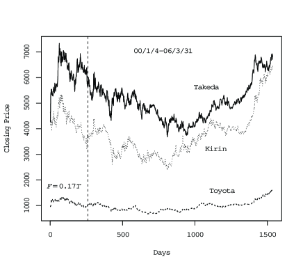
Figure 1: Closing prices

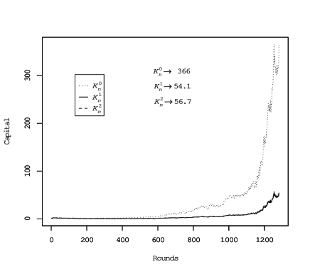
Figure 2: Capital processes

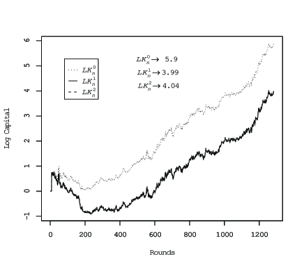
Figure 3: Log capital processes

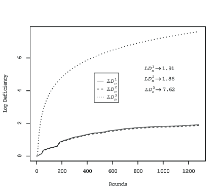
Figure 4: Log deficiency processes

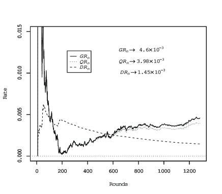
Figure 5: Rate processes

Figure 6 : Closing prices of Takeda, Toyota,

Kirin $F=0.25T$

Figure 7 : Capital processes

$K_{n}^{0},\ K_{n}^{1},\ K_{n}^{2}$

Figure 8 : Log capital processes

$LK_{n}^{0},\ LK_{n}^{1},\ LK_{n}^{2}$

Figure 9 : Log deficiency processes

$LD_{n}^{1},\ LD_{n}^{2},\ LD_{n}^{3}$

Figure 10 : Rate processes

$GR_{n},\ QR_{n},\ DR_{n}$

Figure 6: Closing prices

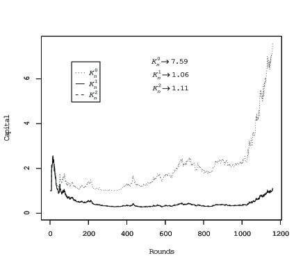
Figure 7: Capital processes

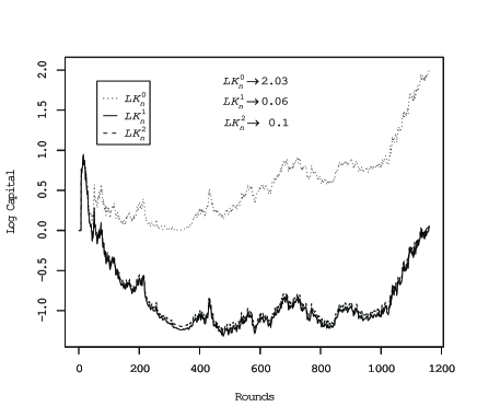
Figure 8: Log capital processes

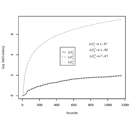
Figure 9: Log deficiency processes

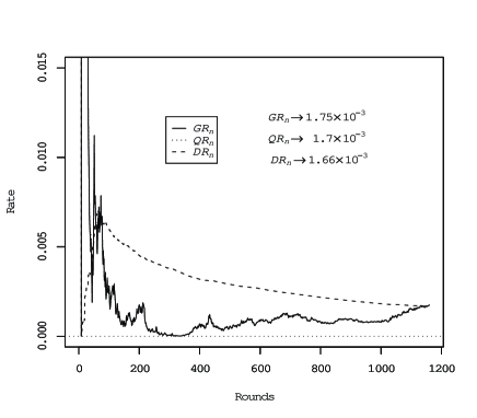
Figure 10: Rate processes

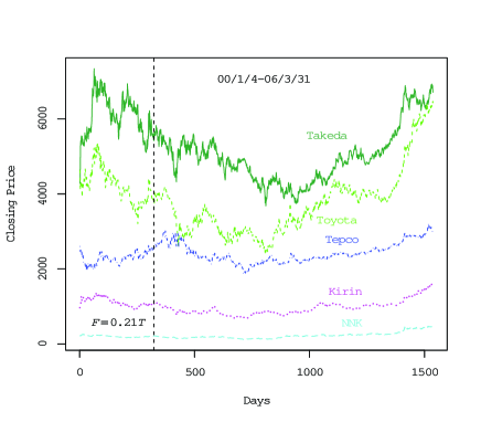
Figure 11: Closing prices

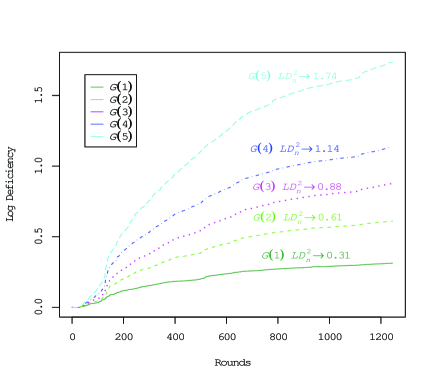
Figure 12: Log deficiency processes $LD_{n}^{2}$

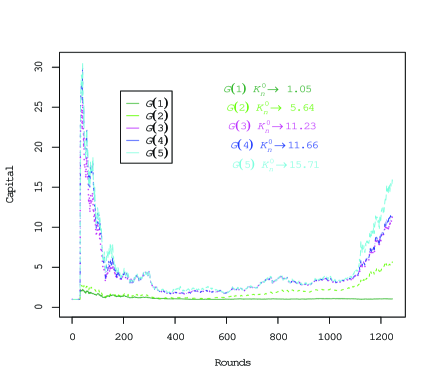
Figure 13: Capital processes $K_{n}^{0}$

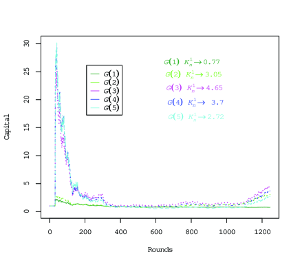
Figure 14: Capital processes $K_{n}^{1}$

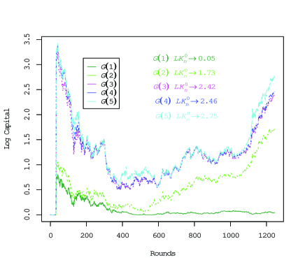
Figure 15: Log capital processes $LK_{n}^{0}$

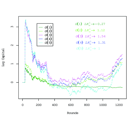
Figure 16: Log capital processes $LK_{n}^{1}$

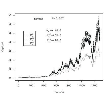
Figure 17: $K_{n}^{1},\ K_{n}^{U0},\ K_{n}^{U1}$

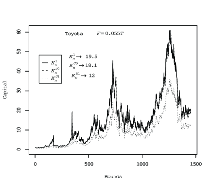
Figure 18: $K_{n}^{1},\ K_{n}^{U0},\ K_{n}^{U1}$

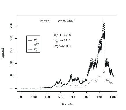
Figure 19: $K_{n}^{1},\ K_{n}^{U0},\ K_{n}^{U1}$

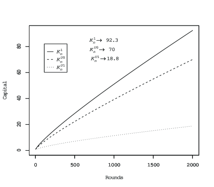
Figure 20: $K_{n}^{1},\ K_{n}^{U0},\ K_{n}^{U1}$

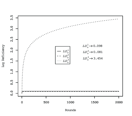
Figure 21: Log deficiency processes

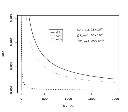
Figure 22: Rate processes

7 Some discussions

In this paper we proposed a sequential optimizing strategy in multi-dimensional bounded forecasting game and showed that it is a very flexible strategy. From a theoretical viewpoint it allowed us to prove a generalized form of the strong law of large numbers. From a practical viewpoint the strategy is easy to implement even in high dimensions and its performance is competitive against universal portfolio.

Theoretical comparison of our strategy with universal portfolio needs more detailed asymptotic investigation of the capital processes of these strategies. This is left to our future research.

In Section 4 as a limit order type strategy we considered successive stopping times defined by a sphere of radius $\delta$ for the vector of returns (cf. (23)), which is based on the standard Euclidean norm in ${\mathbb{R}}^{d}$. We note that other boundaries based on other norms which are equivalent to the standard one provide the same result stated in Theorem 4.1.

Theorem 2.1 for the case of $\sup_{N}V_{N}<\infty$ does not provide a game-theoretic version of Kolmogorov’s three series theorem. It only implies that $S_{N}$, $N=1,2,\dots$, are bounded. However we expect that a game-theoretic version of Kolmogorov’s three series theorem can be established by appropriate modification of our strategy. This topic is also left to our future research.

Appendix A A convergence lemma

Let $u_{1},u_{2},\dots$ be a sequence of points in ${\mathbb{R}}^{d}$. We assume that they are bounded: $\|u_{n}\|\leq 1$, $\forall n$, and that $u_{1},\dots,u_{d}$ are linearly independent. Define

$$y_{n}=(u_{1}u_{1}^{\mathrm{t}}+u_{2}u_{2}^{\mathrm{t}}+\dots+u_{n-1}u_{n-1}^{\mathrm{t}})^{-1}u_{n}\in{\mathbb{R}}^{d}.$$

Then we have the following lemma. It is trivial for $d=1$, but for $d>1$ we need a careful argument.

Lemma A.1.

$$y_{n}\rightarrow 0,\qquad(n\rightarrow\infty).$$

Proof.

We first show that $y_{n}$ is bounded. Let $\lambda_{\min,d}>0$ denote the minimum eigenvalue of $u_{1}u_{1}^{\mathrm{t}}+\cdots+u_{d}u_{d}^{\mathrm{t}}$. Then all the eigenvalues of $u_{1}u_{1}^{\mathrm{t}}+\cdots+u_{n}u_{n}^{\mathrm{t}}$, $n\geq d$, are greater then equal to $\lambda_{\min,d}$. Then all the eigenvalues of $(u_{1}u_{1}^{\mathrm{t}}+\cdots+u_{n}u_{n}^{\mathrm{t}})^{-2}$ are less than or equal to $\lambda_{\min,d}^{-2}$. Hence

$$\|y_{n}\|^{2}\leq\lambda_{\min,d}^{-2}\|u_{n}\|^{2}$$ (30)

and $y_{n}$, $n=1,2,\dots$, are bounded.

Now we argue by contradiction. Suppose that $y_{n}$, $n=1,2,\dots$, do not converge to zero. Then there exists a subsequence $n_{k}$, $k=1,2,\dots$ such that $y_{n_{k}}\rightarrow a\neq 0$, $(k\rightarrow\infty)$. In view of (30), if $u_{n_{k}}\rightarrow 0$ then $y_{n_{k}}\rightarrow 0$, which is a contradiction. Therefore $u_{n_{k}}$, $k=1,2,\dots$, do not converge to 0. Then there exists a further subsequence $\{\tilde{n}_{k}\}\subset\{n_{k}\}$ such that $u_{\tilde{n}_{k}}\rightarrow b\neq 0$. Then $y_{\tilde{n}_{k}}\rightarrow a$, $u_{\tilde{n}_{k}}\rightarrow b$. Consider

$$(u_{1}u_{1}^{\mathrm{t}}+\dots+u_{\tilde{n}_{k}-1}u_{\tilde{n}_{k}-1}^{\mathrm{t}})y_{\tilde{n}_{k}}=u_{\tilde{n}_{k}}.$$

Then

$$(u_{1}u_{1}^{\mathrm{t}}+\dots+u_{\tilde{n}_{k}-1}u_{\tilde{n}_{k}-1}^{\mathrm{t}})y_{\tilde{n}_{k}}\rightarrow b.$$

Multiplying by $y_{\tilde{n}_{k}}^{\mathrm{t}}$ from the left we have

$$y_{\tilde{n}_{k}}^{\mathrm{t}}(u_{1}u_{1}^{\mathrm{t}}+\dots+u_{\tilde{n}_{k}-1}u_{\tilde{n}_{k}-1}^{\mathrm{t}})y_{\tilde{n}_{k}}=y_{\tilde{n}_{k}}^{\mathrm{t}}u_{\tilde{n}_{k}}\rightarrow a^{\mathrm{t}}b.$$

Now the left-hand side is written as

$$(y_{\tilde{n}_{k}}^{\mathrm{t}}u_{1})^{2}+\dots+(y_{\tilde{n}_{k}}^{\mathrm{t}}u_{\tilde{n}_{k}-1})^{2}.$$

Note that for sufficiently large $k,k^{\prime}$, $(y_{\tilde{n}_{k}}^{\mathrm{t}}u_{\tilde{n}_{k^{\prime}}})^{2}$ are all close to $(b^{\mathrm{t}}a)^{2}$. Since we have infinitely many such terms, the left-hand side diverges to $\infty$ if $b^{\mathrm{t}}a\neq 0$. This contradicts the fact that the right-hand side converges to a finite value. Therefore $b^{\mathrm{t}}a=0$. But then

$$\liminf(y_{\tilde{n}_{k}}^{\mathrm{t}}u_{1})^{2}+\dots+(y_{\tilde{n}_{k}}^{\mathrm{t}}u_{\tilde{n}_{k}-1})^{2}\geq(y_{\tilde{n}_{k}}^{\mathrm{t}}u_{1})^{2}+\dots+(y_{\tilde{n}_{k}}^{\mathrm{t}}u_{d})^{2}$$

$$\qquad\rightarrow(a^{\mathrm{t}}u_{1})^{2}+\dots+(a^{\mathrm{t}}u_{d})^{2}>0,$$

which is again a contradiction. ∎

We also present the following corollary of the above lemma.

Corollary A.1.

With the same notation and conditions as in Lemma 3.1

$$\tilde{y}_{n}=(u_{1}u_{1}^{\mathrm{t}}+u_{2}u_{2}^{\mathrm{t}}+\dots+u_{n-1}u_{n-1}^{\mathrm{t}})^{-1/2}u_{n}\rightarrow 0,\quad(n\rightarrow\infty).$$

This corollary follows easily from the fact that $\|\tilde{y}_{n}\|^{2}=u_{n}^{\mathrm{t}}y_{n}$ and $u_{n}$ is bounded.

Based on the above corollary we give a proof of Lemma 3.1. Before going into the proof, we summarize some facts on matrix inequalities. For a symmetric matrix $A$, let $A>0$ mean that $A$ is positive definite. If $A\geq B>0$, then $B^{-1}\geq A^{-1}>0$ (Lemma 4.2 of [2]). Note that $A\geq B\geq 0$ does not imply $A^{2}\geq B^{2}$ (e.g. Chapter 1 of [17]), which complicates our proof.

Proof of Lemma 3.1.

By the definition of $C_{1}$ in (15) we have

$$V_{0,n-1}(\alpha_{n-1}^{*},\alpha_{n}^{*})\geq\frac{1}{C_{1}^{2}}V_{0,n-1}(0,0),$$

where $V_{0,n-1}(0,0)=\sum_{i=-n_{0}+1}^{n}x_{i}x_{i}^{\mathrm{t}}$ is positive definite because of the training data. Write

$$\Delta\alpha_{n}^{*}=V_{0,n-1}(\alpha_{n-1}^{*},\alpha_{n}^{*})^{-1/2}V_{0,n-1}(\alpha_{n-1}^{*},\alpha_{n}^{*})^{-1/2}x_{n}(\alpha_{n-1}^{*}).$$

Then

$$\|\Delta\alpha_{n}^{*}\|^{2}\leq\frac{x_{n}(\alpha_{n}^{*})^{\mathrm{t}}V_{0,n-1}(\alpha_{n-1}^{*},\alpha_{n}^{*})^{-1}x_{n}(\alpha_{n}^{*})}{\lambda_{\min,0,n-1}(\alpha_{n-1}^{*},\alpha_{n}^{*})},$$

where $\lambda_{\min,0,n-1}(\alpha_{n-1}^{*},\alpha_{n}^{*})$ is the minimum eigenvalue of $V_{0,n-1}(\alpha_{n-1}^{*},\alpha_{n}^{*})$. Let $\lambda_{\min,0,0}$ denote the minimum eigenvalue of $V_{0,0}$. Then $\lambda_{\min,0,n-1}(\alpha_{n-1}^{*},\alpha_{n}^{*})\geq\lambda_{\min,0,0}/C_{1}^{2}$ for all $n\geq 1$ and

$$\|\Delta\alpha_{n}^{*}\|^{2}\leq\frac{C_{1}^{2}}{\lambda_{\min,0,0}}x_{n}(\alpha_{n}^{*})^{\mathrm{t}}V_{0,n-1}(\alpha_{n-1}^{*},\alpha_{n}^{*})^{-1}x_{n}(\alpha_{n}^{*}).$$

For $n\geq 1$, $1+\alpha_{n}^{*}\cdot x_{n}\geq\epsilon_{0}$. Hence

$$\|\Delta\alpha_{n}^{*}\|^{2}\leq\frac{C_{1}^{2}}{\epsilon_{0}^{2}\lambda_{\min,0,0}}x_{n}^{\mathrm{t}}V_{0,n-1}(\alpha_{n-1}^{*},\alpha_{n}^{*})^{-1}x_{n}\leq\frac{C_{1}^{4}}{\epsilon_{0}^{2}\lambda_{\min,0,0}}x_{n}^{\mathrm{t}}V_{0,n-1}(0,0)^{-1}x_{n}.$$

The right-hand side converges to 0 by Corollary A.1. ∎

References

- [1] T. W. Anderson. An Introduction to Multivariate Statistical Analysis. 3rd ed., Wiley, Hoboken, New Jersey, 2003.
- [2] T. W. Anderson and A. Takemura. A new proof of admissibility of tests in the multivariate analysis of variance. Journal of Multivariate Analysis, 12, 457–478, 1982.
- [3] Thomas M. Cover. Universal portfolios. Mathematical Finance, 1, (1), 1-29, 1991.
- [4] Thomas M. Cover and E. Ordentlich. Universal portfolios with side information. IEEE Trans. Inf. Theory, IT-42, 348-363, 1996.
- [5] E. Ordentlich and Thomas M. Cover. The cost of achieving the best portfolio in hindsight. Math. Operations Res., 23, (4), 960-982, 1998.
- [6] Thomas M. Cover and Joy A. Thomas. Elements of Information Theory. 2nd ed., Wiley, New York, 2006.
- [7] John L. Kelly. A new interpretation of information rate. Bell System Technical Journal, 35, 917–26, 1956.
- [8] Masayuki Kumon and Akimichi Takemura. On a simple strategy weakly forcing the strong law of large numbers in the bounded forecasting game. Annals of the Institute of Statistical Mathematics, 60, 801–812, 2008.
- [9] Masayuki Kumon, Akimichi Takemura and Kei Takeuchi. Capital process and optimality properties of a Bayesian Skeptic in coin-tossing games. Stochastic Analysis and Applications, 26, 1161–1180, 2008.
- [10] Glenn Shafer and Vladimir Vovk. Probability and Finance: It’s Only a Game! Wiley, New York, 2001.
- [11] Albert N. Shiryaev. Probability. Second edition. Springer, New York, 1996.
- [12] Kei Takeuchi, Masayuki Kumon and Akimichi Takemura. A new formulation of asset trading games in continuous time with essential forcing of variation exponent. arXiv:0708.0275v1, 2007. To appear in Bernoulli.
- [13] Kei Takeuchi, Masayuki Kumon and Akimichi Takemura. Multistep Bayesian strategy in coin-tossing games and its application to asset trading games in continuous time. arXiv:0802.4311v2, 2008. Submitted for publication.
- [14] Vladimir Vovk. Continuous-time trading and the emergence of randomness. Stochastics, 81, 455–466, 2009.
- [15] Vladimir Vovk. Continuous-time trading and the emergence of volatility Elect. Comm. in Probab. 13, 319–324, 2008.
- [16] Vladimir Vovk. Continuous-time trading and the emergence of probability. arXiv:0904.4364v1, 2009.
- [17] Xingzhi Zhan. Matrix Inequalities. Springer, Berlin, 2002.