Combined CDF and D0 Upper Limits on Standard Model Higgs-Boson Production with 2.1 - 5.4 fb^-1 of Data

Abstract

We combine results from CDF and D0 on direct searches for a standard model (SM) Higgs boson ($H$) in $p\bar{p}$ collisions at the Fermilab Tevatron at $\sqrt{s}=1.96$ TeV. Compared to the previous Tevatron Higgs search combination more data have been added and some previously used channels have been reanalyzed to gain sensitivity. We use the latest parton distribution functions and $gg\rightarrow H$ theoretical cross sections when comparing our limits to the SM predictions. With 2.0-4.8 fb^-1 of data analyzed at CDF, and 2.1-5.4 fb^-1 at D0, the 95% C.L. upper limits on Higgs boson production are a factor of 2.70 (0.94) times the SM cross section for a Higgs boson mass of $m_{H}=$115 (165) GeV/$c^{2}$. The corresponding median upper limits expected in the absence of Higgs boson production are 1.78 (0.89). The mass range excluded at 95% C.L. for a SM Higgs is $163<m_{H}<166$ GeV/$c^{2}$, with an expected exclusion of $159<m_{H}<168$ GeV/$c^{2}$.
                                               Preliminary Results

I Introduction

The search for a mechanism for electroweak symmetry breaking, and in particular for a standard model (SM) Higgs boson has been a major goal of particle physics for many years, and is a central part of the Fermilab Tevatron physics program. Both the CDF and D0 experiments have performed new combinations CDFHiggs ; DZHiggs of multiple direct searches for the SM Higgs boson. The new searches include more data and improved analysis techniques compared to previous analyses. The sensitivities of these new combinations significantly exceed those of previous combinations prevhiggs .

In this note, we combine the most recent results of all such searches in $p\bar{p}$ collisions at $\sqrt{s}=1.96$ TeV. The analyses combined here seek signals of Higgs bosons produced in association with vector bosons ($q\bar{q}\rightarrow W/ZH$), through gluon-gluon fusion ($gg\rightarrow H$), and through vector boson fusion (VBF) ($q\bar{q}\rightarrow q^{\prime}\bar{q}^{\prime}H$) corresponding to integrated luminosities ranging from 2.0 to 4.8 fb^-1 at CDF and 2.1 to 5.4 fb^-1 at D0. The Higgs boson decay modes studied are $H\rightarrow b{\bar{b}}$, $H\rightarrow W^{+}W^{-}$, $H\rightarrow\tau^{+}\tau^{-}$ and $H\rightarrow\gamma\gamma$.

To simplify the combination, the searches are separated into 90 mutually exclusive final states (36 for CDF and 54 for D0; see Table 2 and  3) referred to as “analyses” in this note. The selection procedures for each analysis are detailed in Refs. cdfWH2J through dzttH , and are briefly described below.

II Acceptance, Backgrounds, and Luminosity

Event selections are similar for the corresponding CDF and D0 analyses. For the case of $WH\rightarrow\ell\nu b\bar{b}$, an isolated lepton ($\ell=$ electron or muon) and two jets are required, with one or more $b$-tagged jet, i.e., identified as containing a weakly-decaying $B$ hadron. Selected events must also display a significant imbalance in transverse momentum (referred to as missing transverse energy or $E\kern-5.70007pt\raise 0.81805pt\hbox{/}_{T}$). Events with more than one isolated lepton are vetoed. For the D0 $WH\rightarrow\ell\nu b\bar{b}$ analyses, two and three jet events are analyzed separately, and in each of these samples two non-overlapping $b$-tagged samples are defined, one being a single “tight” $b$-tag (ST) sample, and the other a double “loose” $b$-tag (DT) sample. The tight and loose $b$-tagging criteria are defined with respect to the mis-identification rate that the $b$-tagging algorithm yields for light quark or gluon jets (“mistag rate”) typically $\leq 0.5\%$ or $\leq 1.5\%$, respectively. The final variable is a neural network output which takes as input seven kinematic variables for the two-jet sample, while for the three-jet sample the dijet invariant mass is used.

For the CDF $WH\rightarrow\ell\nu b\bar{b}$ analyses, the events are analyzed in two- and three-jet subsamples separately, and in each of these samples the events are grouped into various lepton and $b$-tag categories. In addition to the selections requiring an identified lepton, events with an isolated track failing lepton selection requirements in the two-jet sample, or an identified loose muon in the extended muon coverage in the three-jet sample, are grouped into their own categories. This provides some acceptance for single prong tau decays. Within the lepton categories there are four $b$-tagging categories considered in the two-jets sample – two tight $b$-tags (TDT), one tight $b$-tag and one loose $b$-tag (LDT), one tight $b$-tag and one looser $b$-tag (LDTX), and a single, tight, $b$- tag (ST). These $b$-tag category names are also used in the three-jets, ${\mbox{$E\kern-5.70007pt\raise 0.81805pt\hbox{/}_{T}$}}b{\bar{b}}$, and $\ell^{+}\ell^{-}b{\bar{b}}$ channel descriptions, except the LDTX events are included in ST events where the looser $b$- tag is ignored. A Bayesian neural network discriminant is trained at each $m_{H}$ in the test range for the two-jet sample, separately for each category, while for the three-jet sample a matrix element discriminant is used.

For the $ZH\rightarrow\nu\bar{\nu}b\bar{b}$ analyses, the selection is similar to the $WH$ selection, except all events with isolated leptons are vetoed and stronger multijet background suppression techniques are applied. Both CDF and D0 analyses use a track-based missing transverse momentum calculation as a discriminant against false $E\kern-5.70007pt\raise 0.81805pt\hbox{/}_{T}$. In addition, D0 trains a boosted decision tree to discriminate against the multijet background. There is a sizable fraction of the $WH\rightarrow\ell\nu b\bar{b}$ signal in which the lepton is undetected that is selected in the $ZH\rightarrow\nu\bar{\nu}b\bar{b}$ samples, so these analyses are also referred to as $VH\rightarrow{\mbox{$E\kern-5.70007pt\raise 0.81805pt\hbox{/}_{T}$}}b\bar{b}$. The CDF analysis uses three non-overlapping samples of events (TDT, LDT and ST as for $WH$). D0 uses orthogonal ST and tight-loose double-tag (TLDT) channels. CDF uses neural-network discriminants as the final variables, while D0 uses boosted decision trees as the advanced analysis technique.

The $ZH\rightarrow\ell^{+}\ell^{-}b\bar{b}$ analyses require two isolated leptons and at least two jets. D0’s $ZH\rightarrow\ell^{+}\ell^{-}b\bar{b}$ analyses separate events into non-overlapping samples of events with one tight $b$-tag (ST) and two loose $b$-tags (DT). CDF separates events into ST, TDT, and LDT samples. For the D0 analysis boosted decision trees provide the final variables for setting limits, while CDF uses the output of a two-dimensional neural network. For this combination D0 has increased the signal acceptance by loosening the selection criteria for one of the leptons. In addition a kinematic fit is now applied to the $Z-$boson and jets. CDF corrects jet energies for $E\kern-5.70007pt\raise 0.81805pt\hbox{/}_{T}$ using a neural network approach. In this analysis the events are divided into three tagging categories: tight double tags, loose double tags, and single tags. Both CDF and D0 further subdivide the channels into lepton categories with different signal-to-background characteristics.

For the $H\rightarrow W^{+}W^{-}$ analyses, signal events are characterized by a large $E\kern-5.70007pt\raise 0.81805pt\hbox{/}_{T}$ and two opposite-signed, isolated leptons. The presence of neutrinos in the final state prevents the reconstruction of the candidate Higgs boson mass. D0 selects events containing electrons and muons, dividing the data sample into three final states: $e^{+}e^{-}$, $e^{\pm}\mu^{\mp}$, and $\mu^{+}\mu^{-}$. CDF separates the $H\rightarrow W^{+}W^{-}$ events in six non-overlapping samples, labeled “high $s/b$” and “low $s/b$” for the lepton selection categories, and also split by the number of jets: 0, 1, or 2+ jets. The sample with two or more jets is not split into low $s/b$ and high $s/b$ lepton categories. The sixth CDF channel is a new low dilepton mass ($m_{\ell^{+}\ell^{-}}$) channel, which accepts events with $m_{\ell^{+}\ell^{-}}<16$ GeV. This channel increases the sensitivity of the $H\rightarrow W^{+}W^{-}$ analyses at low $m_{H}$, adding 10% additional acceptance at $m_{H}=120$ GeV. CDF’s division of events into jet categories allows the analysis discriminants to separate three different categories of signals from the backgrounds more effectively. The signal production mechanisms considered are $gg\rightarrow H\rightarrow W^{+}W^{-}$, $WH+ZH\rightarrow jjW^{+}W^{-}$, and the vector-boson fusion process. For $gg\rightarrow H$, however, recent work anastasiouwebber indicates that the theoretical uncertainties due to scale and PDF variations are significantly different in the different jet categories. CDF and D0 now divide the theoretical uncertainty on $gg\rightarrow H$ into PDF and scale pieces, and use the differential uncertainties of anastasiouwebber . D0 uses neural-networks, including the number of jets as an input, as the final discriminant. CDF likewise uses neural-networks, including likelihoods constructed from matrix-element probabilities (ME) as input in the 0-jet bin. All analyses in this channel have been updated with more data and analysis improvements.

The CDF collaboration also contributes an analysis searching for Higgs bosons decaying to a tau lepton pair, in three separate production channels: direct $gg\rightarrow H$ production, associated $WH$ or $ZH$ production, or vector boson production with $H$ and forward jets in the final state. Two jets are required in the event selection. In this analysis, the final variable for setting limits is a combination of several neural-network discriminants. The theoretical systematic uncertainty on the $gg\rightarrow H$ production rate now takes into account recent theoretical work anastasiouwebber which provides uncertainties in each jet category.

D0 also contributes an analysis for the final state $\tau\tau$ jet jet, which is sensitive to the $VH\rightarrow jj\tau\tau$, $ZH\rightarrow\tau\tau b\bar{b}$, VBF and gluon gluon fusion (with two additional jets) mechanisms. A neural network output is used as the discriminant variable for RunIIa (the first 1.0 fb^-1 of data), while a boosted decision tree output is used for later data.

The CDF collaboration introduces a new all-hadronic channel, $WH+ZH\rightarrow jjb{\bar{b}}$ for this combination. Events are selected with four jets, at least two of which are $b$-tagged with the tight $b$-tagger. The large QCD backgrounds are estimated with the use of data control samples, and the final variable is a matrix element signal probability discriminant.

The D0 collaboration contributes three $WH\rightarrow WW^{+}W^{-}$ analyses, where the associated $W$ boson and the $W$ boson from the Higgs boson decay that has the same charge are required to decay leptonically, thereby defining three like-sign dilepton final states ($e^{\pm}e^{\pm}$, $e^{\pm}\mu^{\pm}$, and $\mu^{\pm}\mu^{\pm}$) containing all decays of the third $W$ boson. In this analysis the final variable is a likelihood discriminant formed from several topological variables. CDF contributes a $WH\rightarrow WW^{+}W^{-}$ analysis using a selection of like-sign dileptons and a neural network to further purify the signal.

D0 also contributes an analysis searching for direct Higgs boson production decaying to a photon pair in 4.2 fb^-1 of data. In this analysis, the final variable is the invariant mass of the two-photon system. Finally, D0 includes the channel $t\bar{t}H\rightarrow t\bar{t}b\bar{b}$. Here the samples are analyzed independently according to the number of $b$-tagged jets (1,2,3, i.e. ST,DT,TT) and the total number of jets (4 or 5). The total transverse energy of the reconstructed objects ($H_{T}$) is used as discriminant variable.

We normalize our Higgs boson signal predictions to the most recent high-order calculations available. The $gg\rightarrow H$ production cross section is calculated at NNLL in QCD and also includes two-loop electroweak effects; see Refs. anastasiou ; grazzinideflorian and references therein for the different steps of these calculations. The newer calculation includes a more thorough treatment of higher-order radiative corrections, particularly those involving $b$ quark loops. The $gg\rightarrow H$ production cross section depends strongly on the PDF set chosen and the accompanying value of $\alpha_{s}$. The cross sections used here are calculated with the MSTW 2008 NNLO PDF set mstw2008 . The new $gg\rightarrow H$ cross sections supersede those used in the update of Summer 2008 TevHiggsICHEP ; nnlo1 ; aglietti , which had a simpler treatment of radiative corrections and used the older MRST 2002 PDF set mrst2002 . The Higgs boson production cross sections used here are listed in Table 1 grazzinideflorian . Furthermore, we now include the larger theoretical uncertainties due to scale variations and PDF variations separately for each jet bin for the $gg\rightarrow H$ processes as evaluated in anastasiouwebber . We treat the scale uncertainties as 100% correlated between jet bins and between CDF and D0, and also treat the PDF uncertainties in the cross section as correlated between jet bins and between CDF and D0. We include all significant Higgs production modes in the high mass search. Besides gluon-gluon fusion through a virtual top quark loop (ggH), we include production in association with a $W$ or $Z$ vector boson (VH) nnlo2 ; Brein ; Ciccolini , and vector boson fusion (VBF) nnlo2 ; Berger . In order to predict the distributions of the kinematics of Higgs boson signal events, CDF and D0 use the PYTHIA pythia Monte Carlo program, with CTEQ5L or CTEQ6L cteq leading-order (LO) parton distribution functions. The Higgs boson decay branching ratio predictions are calculated with HDECAY hdecay , and are also listed in Table 1.

For both CDF and D0, events from multijet (instrumental) backgrounds (“QCD production”) are measured in independent data samples using several different methods. For CDF, backgrounds from SM processes with electroweak gauge bosons or top quarks were generated using PYTHIA, ALPGEN alpgen , MC@NLO MC@NLO and HERWIG herwig programs. For D0, these backgrounds were generated using PYTHIA, ALPGEN, and COMPHEP comphep , with PYTHIA providing parton-showering and hadronization for all the generators. These background processes were normalized using either experimental data or next-to-leading order calculations (including MCFM mcfm for $W+$ heavy flavor process).

Table 1: The (N)NLO production cross sections and decay branching fractions for the SM Higgs boson assumed for the combination

$m_{H}$	$\sigma_{gg\rightarrow H}$	$\sigma_{WH}$	$\sigma_{ZH}$	$\sigma_{\rm{VBF}}$	$B(H\rightarrow b{\bar{b}})$	$B(H\rightarrow\tau^{+}{\tau^{-}})$	$B(H\rightarrow W^{+}W^{-})$
(GeV/$c^{2}$)	(fb)	(fb)	(fb)	(fb)	(%)	(%)	(%)
100	1861	286.1	166.7	99.5	81.21	7.924	1.009
105	1618	244.6	144.0	93.3	79.57	7.838	2.216
110	1413	209.2	124.3	87.1	77.02	7.656	4.411
115	1240	178.8	107.4	79.1	73.22	7.340	7.974
120	1093	152.9	92.7	71.6	67.89	6.861	13.20
125	967	132.4	81.1	67.4	60.97	6.210	20.18
130	858	114.7	70.9	62.5	52.71	5.408	28.69
135	764	99.3	62.0	57.6	43.62	4.507	38.28
140	682	86.0	54.2	52.6	34.36	3.574	48.33
145	611	75.3	48.0	49.2	25.56	2.676	58.33
150	548	66.0	42.5	45.7	17.57	1.851	68.17
155	492	57.8	37.6	42.2	10.49	1.112	78.23
160	439	50.7	33.3	38.6	4.00	0.426	90.11
165	389	44.4	29.5	36.1	1.265	0.136	96.10
170	349	38.9	26.1	33.6	0.846	0.091	96.53
175	314	34.6	23.3	31.1	0.663	0.072	95.94
180	283	30.7	20.8	28.6	0.541	0.059	93.45
185	255	27.3	18.6	26.8	0.420	0.046	83.79
190	231	24.3	16.6	24.9	0.342	0.038	77.61
195	210	21.7	15.0	23.0	0.295	0.033	74.95
200	192	19.3	13.5	21.2	0.260	0.029	73.47

Tables 2 and 3 summarize, for CDF and D0 respectively, the integrated luminosities, the Higgs boson mass ranges over which the searches are performed, and references to further details for each analysis.

Table 2: Luminosity, explored mass range and references for the different processes and final state ($\ell=e,\mu$) for the CDF analyses

Channel	Luminosity (fb-1)	$m_{H}$ range (GeV/$c^{2}$)	Reference
$WH\rightarrow\ell\nu b\bar{b}$ 2-jet channels   3$\times$(TDT,LDT,ST,LDTX)	4.3	100-150	cdfWH2J
$WH\rightarrow\ell\nu b\bar{b}$ 3-jet channels   2$\times$(TDT,LDT,ST)	4.3	100-150	cdfWH3J
$ZH\rightarrow\nu\bar{\nu}b\bar{b}$    (TDT,LDT,ST)	3.6	105-150	cdfmetbb
$ZH\rightarrow\ell^{+}\ell^{-}b\bar{b}$    (low,high $s/b$)$\times$(TDT,LDT,ST)	4.1	100-150	cdfZHll
$H\rightarrow W^{+}W^{-}$    (low,high $s/b$)$\times$(0,1 jets)+(2+ jets)+Low-$m_{\ell\ell}$	4.8	110-200	cdfHWW
$WH\rightarrow WW^{+}W^{-}\rightarrow\ell^{\pm}\nu\ell^{\pm}\nu$	4.8	110-200	cdfHWW
$H$ + $X\rightarrow\tau^{+}\tau^{-}$ + 2 jets	2.0	110-150	cdfHtt
$WH+ZH\rightarrow jjb{\bar{b}}$	2.0	100-150	cdfjjbb

Table 3: Luminosity, explored mass range and references for the different processes and final state ($\ell=e,\mu$) for the D0 analyses

Channel	Luminosity (fb-1)	$m_{H}$ range (GeV/$c^{2}$)	Reference
$WH\rightarrow\ell\nu b\bar{b}$    2$\times$(ST,DT)	5.0	100-150	dzWHl
$VH\rightarrow\tau\tau b\bar{b}/q\bar{q}\tau\tau$	4.9	105-145	dzVHt1 ; dzVHt2
$ZH\rightarrow\nu\bar{\nu}b\bar{b}$    (ST,TLDT)	5.2	100-150	dzZHv
$ZH\rightarrow\ell^{+}\ell^{-}b\bar{b}$    2$\times$(ST,DT)	4.2	100-150	dzZHll
$WH\rightarrow WW^{+}W^{-}\rightarrow\ell^{\pm}\nu\ell^{\pm}\nu$	3.6	120-200	dzWWW1 ; dzWWW2
$H\rightarrow W^{+}W^{-}\rightarrow\ell^{\pm}\nu\ell^{\mp}\nu$	5.4	115-200	dzHWW
$H\rightarrow\gamma\gamma$	4.2	100-150	dzHgg
$t\bar{t}H\rightarrow t\bar{t}b\bar{b}$    2$\times$(ST,DT,TT)	2.1	105-155	dzttH

III Distributions of Candidates

All analyses provide binned histograms of the final discriminant variables for the signal and background predictions, itemized separately for each source, and the data. The number of channels combined is large, and the number of bins in each channel is large. Therefore, the task of assembling histograms and checking whether the expected and observed limits are consistent with the input predictions and observed data is difficult. We therefore provide histograms that aggregate all channels’ signal, background, and data together. In order to preserve most of the sensitivity gain that is achieved by the analyses by binning the data instead of collecting them all together and counting, we aggregate the data and predictions in narrow bins of signal-to-background ratio, $s/b$. Data with similar $s/b$ may be added together with no loss in sensitivity, assuming similar systematic errors on the predictions. The aggregate histograms do not show the effects of systematic uncertainties, but instead compare the data with the central predictions supplied by each analysis.

The range of $s/b$ is quite large in each analysis, and so $\log_{10}(s/b)$ is chosen as the plotting variable. Plots of the distributions of $\log_{10}(s/b)$ are shown for $m_{H}=115$ and 165 GeV/$c^{2}$ in Figure 1. These distributions can be integrated from the high-$s/b$ side downwards, showing the sums of signal, background, and data for the most pure portions of the selection of all channels added together. These integrals can be seen in Figure 2. The most significant candidates are be found in the bins with the highest $s/b$; an excess in these bins relative to the background prediction drives the Higgs boson cross section limit upwards, while a deficit drives it downwards. The lower-$s/b$ bins show that the modeling of the rates and kinematic distributions of the backgrounds is very good. The integrated plots show the excess of events in the high-$s/b$ bins for the analyses seeking a Higgs boson mass of 115 GeV/$c^{2}$, and a deficit of events in the high-$s/b$ bins for the analyses seeking a Higgs boson of mass 165 GeV/$c^{2}$.

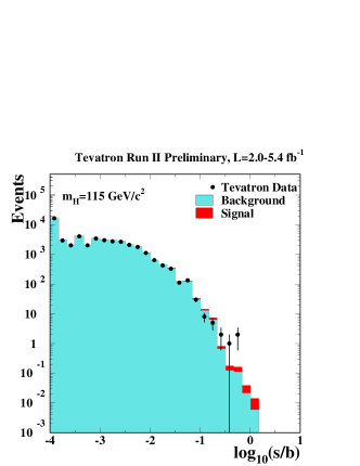
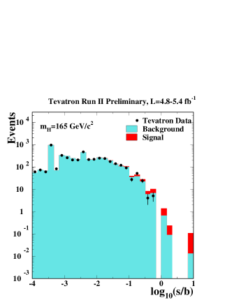
Figure 1: Distributions of $\log_{10}(s/b)$, for the data from all contributing channels from CDF and D0, for Higgs boson masses of 115 and 165 GeV/$c^{2}$. The data are shown with points, and the expected signal is shown stacked on top of the backgrounds. Underflows and overflows are collected into the bottom and top bins.

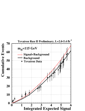
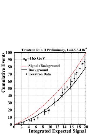
Figure 2: Integrated distributions of $s/b$, starting at the high $s/b$ side. The total signal+background and background-only integrals are shown separately, along with the data sums. Data are only shown for bins that have data events in them.

IV Combining Channels

To gain confidence that the final result does not depend on the details of the statistical formulation, we perform two types of combinations, using the Bayesian and Modified Frequentist approaches, which yield results that agree within 10%. Both methods rely on distributions in the final discriminants, and not just on their single integrated values. Systematic uncertainties enter on the predicted number of signal and background events as well as on the distribution of the discriminants in each analysis (“shape uncertainties”). Both methods use likelihood calculations based on Poisson probabilities.

IV.1 Bayesian Method

Because there is no experimental information on the production cross section for the Higgs boson, in the Bayesian technique CDFHiggs we assign a flat prior for the total number of selected Higgs events. For a given Higgs boson mass, the combined likelihood is a product of likelihoods for the individual channels, each of which is a product over histogram bins:

$${\cal{L}}(R,{\vec{s}},{\vec{b}}|{\vec{n}},{\vec{\theta}})\times\pi({\vec{\theta}})=\prod_{i=1}^{N_{C}}\prod_{j=1}^{Nbins}\mu_{ij}^{n_{ij}}e^{-\mu_{ij}}/n_{ij}!\times\prod_{k=1}^{n_{np}}e^{-\theta_{k}^{2}/2}$$ (1)

where the first product is over the number of channels ($N_{C}$), and the second product is over histogram bins containing $n_{ij}$ events, binned in ranges of the final discriminants used for individual analyses, such as the dijet mass, neural-network outputs, or matrix-element likelihoods. The parameters that contribute to the expected bin contents are $\mu_{ij}=R\times s_{ij}({\vec{\theta}})+b_{ij}({\vec{\theta}})$ for the channel $i$ and the histogram bin $j$, where $s_{ij}$ and $b_{ij}$ represent the expected background and signal in the bin, and $R$ is a scaling factor applied to the signal to test the sensitivity level of the experiment. Truncated Gaussian priors are used for each of the nuisance parameters $\theta_{k}$, which define the sensitivity of the predicted signal and background estimates to systematic uncertainties. These can take the form of uncertainties on overall rates, as well as the shapes of the distributions used for combination. These systematic uncertainties can be far larger than the expected SM signal, and are therefore important in the calculation of limits. The truncation is applied so that no prediction of any signal or background in any bin is negative. The posterior density function is then integrated over all parameters (including correlations) except for $R$, and a 95% credibility level upper limit on $R$ is estimated by calculating the value of $R$ that corresponds to 95% of the area of the resulting distribution.

IV.2 Modified Frequentist Method

The Modified Frequentist technique relies on the $CL_{s}$ method, using a log-likelihood ratio (LLR) as test statistic DZHiggs :

$$LLR=-2\ln\frac{p({\mathrm{data}}|H_{1})}{p({\mathrm{data}}|H_{0})},$$ (2)

where $H_{1}$ denotes the test hypothesis, which admits the presence of SM backgrounds and a Higgs boson signal, while $H_{0}$ is the null hypothesis, for only SM backgrounds. The probabilities $p$ are computed using the best-fit values of the nuisance parameters for each pseudo-experiment, separately for each of the two hypotheses, and include the Poisson probabilities of observing the data multiplied by Gaussian priors for the values of the nuisance parameters. This technique extends the LEP procedure pdgstats which does not involve a fit, in order to yield better sensitivity when expected signals are small and systematic uncertainties on backgrounds are large pflh .

The $CL_{s}$ technique involves computing two $p$-values, $CL_{s+b}$ and $CL_{b}$. The latter is defined by

$$1-CL_{b}=p(LLR\leq LLR_{\mathrm{obs}}|H_{0}),$$ (3)

where $LLR_{\mathrm{obs}}$ is the value of the test statistic computed for the data. $1-CL_{b}$ is the probability of observing a signal-plus-background-like outcome without the presence of signal, i.e. the probability that an upward fluctuation of the background provides a signal-plus-background-like response as observed in data. The other $p$-value is defined by

$$CL_{s+b}=p(LLR\geq LLR_{\mathrm{obs}}|H_{1}),$$ (4)

and this corresponds to the probability of a downward fluctuation of the sum of signal and background in the data. A small value of $CL_{s+b}$ reflects inconsistency with $H_{1}$. It is also possible to have a downward fluctuation in data even in the absence of any signal, and a small value of $CL_{s+b}$ is possible even if the expected signal is so small that it cannot be tested with the experiment. To minimize the possibility of excluding a signal to which there is insufficient sensitivity (an outcome expected 5% of the time at the 95% C.L., for full coverage), we use the quantity $CL_{s}=CL_{s+b}/CL_{b}$. If $CL_{s}<0.05$ for a particular choice of $H_{1}$, that hypothesis is deemed excluded at the 95% C.L.

Systematic uncertainties are included by fluctuating the predictions for signal and background rates in each bin of each histogram in a correlated way when generating the pseudo-experiments used to compute $CL_{s+b}$ and $CL_{b}$.

IV.3 Systematic Uncertainties

Systematic uncertainties differ between experiments and analyses, and they affect the rates and shapes of the predicted signal and background in correlated ways. The combined results incorporate the sensitivity of predictions to values of nuisance parameters, and include correlations between rates and shapes, between signals and backgrounds, and between channels within experiments and between experiments. More on these issues can be found in the individual analysis notes cdfWH2J through dzttH . Here we consider only the largest contributions and correlations between and within the two experiments.

IV.3.1 Correlated Systematics between CDF and D0

The uncertainties on the measurements of the integrated luminosities are 6% (CDF) and 6.1% (D0). Of these values, 4% arises from the uncertainty on the inelastic $p\bar{p}$ scattering cross section, which is correlated between CDF and D0. CDF and D0 also share the assumed values and uncertainties on the production cross sections for top-quark processes ($t\bar{t}$ and single top) and for electroweak processes ($WW$, $WZ$, and $ZZ$). In order to provide a consistent combination, the values of these cross sections assumed in each analysis are brought into agreement. We use $\sigma_{t\bar{t}}=7.88\pm 0.79$ pb, following the calculation of Moch and Uwer mochuwer , assuming a top quark mass $m_{t}=172.4\pm 1.2$ GeV/$c^{2}$ tevtop08 , and using the MRST2006nnlo PDF set mrst2006 . Other calculations of $\sigma_{t\bar{t}}$ are similar otherttbar . We use $\sigma_{\rm{SingleTop}}=3.38\pm 0.34$ pb, following the calculation of Kidonakis kidonakis . Other calculations of $\sigma_{\rm{SingleTop}}$ are similar for our purposes harris . We use $\sigma_{WW}=12.4\pm 0.7$ pb, $\sigma_{WZ}=3.7\pm 0.2$ pb, and $\sigma_{ZZ}=3.8\pm 0.2$ pb, calculated with MCFM mcfm .

In many analyses, the dominant background yields are calibrated with data control samples. The methods of measuring the multijet (“QCD”) backgrounds differ between CDF and D0, and even between analyses within the collaborations, there is no correlation assumed between these rates. Similarly, the large uncertainties on the background rates for $W$+heavy flavor (HF) and $Z$+heavy flavor are considered at this time to be uncorrelated, as both CDF and D0 estimate these rates using data control samples, but employ different techniques. The calibrations of fake leptons, unvetoed $\gamma\rightarrow e^{+}e^{-}$ conversions, $b$-tag efficiencies and mistag rates are performed by each collaboration using independent data samples and methods, hence are considered uncorrelated.

IV.3.2 Correlated Systematic Uncertainties for CDF

The dominant systematic uncertainties for the CDF analyses are shown in Table 4 for the $W^{\pm}H\rightarrow W^{\pm}b{\bar{b}}$ channels, in Table 6 for the $(W,Z)H\rightarrow{\mbox{$E\kern-5.70007pt\raise 0.81805pt\hbox{/}_{T}$}}b{\bar{b}}$ channels, in Table 8 for the $ZH\rightarrow\ell^{+}\ell^{-}b{\bar{b}}$ channels, in Table 10 for the $H\rightarrow W^{+}W^{-}\rightarrow\ell^{\prime\pm}\nu\ell^{\prime\mp}\nu$ channels, in Table 16 for the $H\rightarrow\tau^{+}\tau^{-}$ channel, in Table 17 for the $WH+ZH\rightarrow jjb{\bar{b}}$ channel, and in Table 12 for the $WH\rightarrow WWW\rightarrow\ell^{\prime\pm}\ell^{\prime\pm}$ channel. Each source induces a correlated uncertainty across all CDF channels’ signal and background contributions which are sensitive to that source. For $H\rightarrow b\bar{b}$, the largest uncertainties on signal arise from a scale factor for $b$-tagging (5.3-16%), jet energy scale (1-20%) and MC modeling (2-10%). The shape dependence of the jet energy scale, $b$-tagging and uncertainties on gluon radiation (“ISR” and “FSR”) are taken into account for some analyses (see tables). For $H\rightarrow W^{+}W^{-}$, the largest uncertainty comes from MC modeling (5%). For simulated backgrounds, the uncertainties on the expected rates range from 11-40% (depending on background). The backgrounds with the largest systematic uncertainties are in general quite small. Such uncertainties are constrained by fits to the nuisance parameters, and they do not affect the result significantly. Because the largest background contributions are measured using data, these uncertainties are treated as uncorrelated for the $H\rightarrow b\bar{b}$ channels. For the $H\rightarrow W^{+}W^{-}$ channel, the uncertainty on luminosity is taken to be correlated between signal and background. The differences in the resulting limits when treating the remaining uncertainties as correlated or uncorrelated, is less than $5\%$.

IV.3.3 Correlated Systematic Uncertainties for D0

The dominant systematic uncertainties for D0 analyses are shown in Tables V,7,9,13,14, 15, and 18. Each source induces a correlated uncertainty across all D0 channels sensitive to that source. Wherever appropriate the impact of the systematic effect on both the rate and shape of the predicted signal and background is included. For the low mass, $H\rightarrow b\bar{b}$ analyses, the largest sources of uncertainty originate from the $b$-tagging rate ($\sim$5-10% per tagged jet), the determination of the jet energy, acceptance, and resolution ($\sim$5-10%), the normalization of the W and Z + heavy flavor backgrounds ($\sim$20%) and the determination of the multijet background ($\sim 25\%$). For the $H\rightarrow W^{+}W^{-}$ and $WH\rightarrow WW^{+}W^{-}$analyses, one of the largest uncertainties is associated with the lepton measurement and acceptance, and is $\sim$5-10% depending on the final state. Significant sources for all analyses are the uncertainties on the luminosity and the cross sections for the simulated backgrounds, and are $\sim 6\%$ and 6-10% respectively. All systematic uncertainties arising from the same source are taken to be correlated between the different backgrounds and between signal and background.

Table 4: Systematic uncertainties on the signal and background contributions for CDF’s $WH\rightarrow\ell\nu b{\bar{b}}$ tight (TDT), loose (LDT) double tag, looser (LDTX) double tag, and single tag (ST) channels. Systematic uncertainties are listed by name; see the original references for a detailed explanation of their meaning and on how they are derived. Systematic uncertainties for $WH$ shown in this table are obtained for $m_{H}=115$ GeV/$c^{2}$. Uncertainties are relative, in percent, and are symmetric unless otherwise indicated.

CDF: tight (TDT) and loose (LDT) double-tag $WH\rightarrow\ell\nu b{\bar{b}}$ relative uncertainties (%)

Contribution	$W$+HF	Mistags	Top	Diboson	Non-$W$	$WH$
Luminosity ($\sigma_{\mathrm{inel}}(p{\bar{p}})$)	0	0	3.8	3.8	0	3.8
Luminosity Monitor	0	0	4.4	4.4	0	4.4
Lepton ID	0	0	2	2	0	2
Jet Energy Scale	0	0	0	0	0	2
Mistag Rate	0	35	0	0	0	0
$B$-Tag Efficiency	0	0	8.6	8.6	0	8.6
$t{\bar{t}}$ Cross Section	0	0	10	0	0	0
Diboson Rate	0	0	0	11.5	0	0
Signal Cross Section	0	0	0	0	0	5
HF Fraction in W+jets	45	0	0	0	0	0
ISR+FSR+PDF	0	0	0	0	0	5
QCD Rate	0	0	0	0	40	0

CDF: looser double-tag (LDTX) $WH\rightarrow\ell\nu b{\bar{b}}$ relative uncertainties (%)

Contribution	$W$+HF	Mistags	Top	Diboson	Non-$W$	$WH$
Luminosity ($\sigma_{\mathrm{inel}}(p{\bar{p}})$)	0	0	3.8	3.8	0	3.8
Luminosity Monitor	0	0	4.4	4.4	0	4.4
Lepton ID	0	0	2	2	0	2
Jet Energy Scale	0	0	0	0	0	2.2
Mistag Rate	0	36	0	0	0	0
$B$-Tag Efficiency	0	0	13.6	13.6	0	13.6
$t{\bar{t}}$ Cross Section	0	0	10	0	0	0
Diboson Rate	0	0	0	11.5	0	0
Signal Cross Section	0	0	0	0	0	5
HF Fraction in W+jets	45	0	0	0	0	0
ISR+FSR+PDF	0	0	0	0	0	7.7
QCD Rate	0	0	0	0	40	0

CDF: single tag (ST) $WH\rightarrow\ell\nu b{\bar{b}}$ relative uncertainties (%)

Contribution	$W$+HF	Mistags	Top	Diboson	Non-$W$	$WH$
Luminosity ($\sigma_{\mathrm{inel}}(p{\bar{p}})$)	0	0	3.8	3.8	0	3.8
Luminosity Monitor	0	0	4.4	4.4	0	4.4
Lepton ID	0	0	2	2	0	2
Jet Energy Scale	0	0	0	0	0	2
Mistag Rate	0	35	0	0	0	0
$B$-Tag Efficiency	0	0	4.3	4.3	0	4.3
$t{\bar{t}}$ Cross Section	0	0	10	0	0	0
Diboson Rate	0	0	0	11.5	0	0
Signal Cross Section	0	0	0	0	0	5
HF Fraction in W+jets	42	0	0	0	0	0
ISR+FSR+PDF	0	0	0	0	0	3.0
QCD Rate	0	0	0	0	40	0

Table 5: Systematic uncertainties on the signal contributions for D0’s $WH\rightarrow\ell\nu b{\bar{b}}$ single (ST) and double tag (DT) channels. Systematic uncertainties are listed by name, see the original references for a detailed explanation of their meaning and on how they are derived. Systematic uncertainties for $WH$ shown in this table are obtained for $m_{H}=115$ GeV/$c^{2}$. Uncertainties are relative, in percent, and are symmetric unless otherwise indicated.

D0: Single Tag (ST) $WH\rightarrow\ell\nu b\bar{b}$ analysis relative uncertainties (%)

Contribution	WZ/WW	Wbb/Wcc	Wjj/Wcj	$~{}~{}~{}t\bar{t}~{}~{}~{}$	single top	Multijet	WH
Luminosity	6	6	6	6	6	0	6
Trigger eff.	2–5	2–5	2–5	2–5	2–5	0	2–5
EM ID/Reco eff./resol.	3	3	3	3	3	0	3
Muon ID/Reco eff./resol.	4.1	4.1	4.1	4.1	4.1	0	4.1
Jet ID/Reco eff.	2	2	2	2	2	0	2
Jet Energy Scale	3	3	3	3	3	0	3
Jet mult./frag./modeling	3.5	3.5	3.5	3.5	3.5	0	3.5
$b$-tagging/taggability	4	4	11	4	4	0	4
Cross Section	6	9	9	10	10	0	6
Heavy-Flavor K-factor	0	20	0	0	0	0	0
Instrumental-WH	0	0	0	0	0	26	0

D0: Double Tag (DT) $WH\rightarrow\ell\nu b\bar{b}$ analysis relative uncertainties (%)

Contribution	WZ/WW	Wbb/Wcc	Wjj/Wcj	$~{}~{}~{}t\bar{t}~{}~{}~{}$	single top	Multijet	WH
Luminosity	6	6	6	6	6	0	6
Trigger eff.	2–5	2–5	2–5	2–5	2–5	0	2–5
EM ID/Reco eff./resol.	3	3	3	3	3	0	3
Muon ID/Reco eff./resol.	4.1	4.1	4.1	4.1	4.1	0	4.1
Jet ID/Reco eff.	2	2	2	2	2	0	2
Jet Energy Scale	3	3	3	3	3	0	3
Jet mult./frag./modeling	3.5	3.5	3.5	3.5	3.5	0	3.5
$b$-tagging/taggability	6	6	20	6	6	0	6
Cross Section	6	9	9	10	10	0	6
Heavy-Flavor K-factor	0	20	0	0	0	0	0
Instrumental-WH	0	0	0	0	0	26	0

Table 6: Systematic uncertainties for CDF’s $WH,ZH\rightarrow{\mbox{$E\kern-5.70007pt\raise 0.81805pt\hbox{/}_{T}$}}b{\bar{b}}$ tight (TDT and loose (LDT) double-tag, and single-tag (ST) channels. Systematic uncertainties are listed by name; see the original references for a detailed explanation of their meaning and on how they are derived. Systematic uncertainties for $ZH$ and $WH$ shown in this table are obtained for $m_{H}=120$ GeV/$c^{2}$. Uncertainties are relative, in percent, and are symmetric unless otherwise indicated.

CDF: $WH,ZH\rightarrow{\mbox{$E\kern-5.70007pt\raise 0.81805pt\hbox{/}_{T}$}}b{\bar{b}}$ tight double-tag (TDT) channel relative uncertainties (%)

	ZH	WH	Multijet	Top Pair	S. Top	Di-boson	W + h.f.	Z + h.f.
Correlated uncertainties
Luminosity	3.8	3.8		3.8	3.8	3.8	3.8	3.8
Lumi Monitor	4.4	4.4		4.4	4.4	4.4	4.4	4.4
Tagging SF	8.6	8.6		8.6	8.6	8.6	8.6	8.6
Trigger Eff. (shape)	1.0	1.2	1.1	0.7	1.1	1.6	1.7	1.3
Lepton Veto	2.0	2.0		2.0	2.0	2.0	2.0	2.0
PDF Acceptance	2.0	2.0		2.0	2.0	2.0	2.0	2.0
JES (shape)	${}^{+3.0}_{-3.0}$	${}^{+3.5}_{-4.7}$	${}^{-4.0}_{+3.8}$	${}^{+1.1}_{-1.1}$	${}^{+2.4}_{-4.7}$	${}^{+8.2}_{-6.1}$	${}^{+7.3}_{-11.8}$	${}^{+6.5}_{-8.3}$
ISR	${}^{+4.4}_{+3.7}$
FSR	${}^{+1.8}_{+4.4}$
Uncorrelated uncertainties
Cross-Section	5	5		10	10	11.5	40	40
Multijet Norm. (shape)			17

CDF: $WH,ZH\rightarrow{\mbox{$E\kern-5.70007pt\raise 0.81805pt\hbox{/}_{T}$}}b{\bar{b}}$ loose double-tag (LDT) channel relative uncertainties (%)

	ZH	WH	Multijet	Top Pair	S. Top	Di-boson	W + h.f.	Z + h.f.
Correlated uncertainties
Luminosity	3.8	3.8		3.8	3.8	3.8	3.8	3.8
Lumi Monitor	4.4	4.4		4.4	4.4	4.4	4.4	4.4
Tagging SF	9.1	9.1		9.1	9.1	9.1	9.1	9.1
Trigger Eff. (shape)	1.2	1.3	1.1	0.7	1.2	1.2	1.8	1.3
Lepton Veto	2.0	2.0		2.0	2.0	2.0	2.0	2.0
PDF Acceptance	2.0	2.0		2.0	2.0	2.0	2.0	2.0
JES (shape)	${}^{+3.7}_{-3.7}$	${}^{+4.0}_{-4.0}$	${}^{-5.4}_{+5.2}$	${}^{+1.1}_{-0.7}$	${}^{+4.2}_{-4.2}$	${}^{+7.0}_{-7.0}$	${}^{+1.3}_{-7.6}$	${}^{+6.2}_{-7.1}$
ISR	${}^{+1.4}_{-2.9}$
FSR	${}^{+5.3}_{+2.5}$
Uncorrelated uncertainties
Cross-Section	5.0	5.0		10	10	11.5	40	40
Multijet Norm. (shape)			11

CDF: $WH,ZH\rightarrow{\mbox{$E\kern-5.70007pt\raise 0.81805pt\hbox{/}_{T}$}}b{\bar{b}}$ single-tag (ST) channel relative uncertainties (%)

	ZH	WH	Multijet	Top Pair	S. Top	Di-boson	W + h.f.	Z + h.f.
Correlated uncertainties
Luminosity	3.8	3.8		3.8	3.8	3.8	3.8	3.8
Lumi Monitor	4.4	4.4		4.4	4.4	4.4	4.4	4.4
Tagging SF	4.3	4.3		4.3	4.3	4.3	4.3	4.3
Trigger Eff. (shape)	0.9	1.1	1.1	0.7	1.1	1.3	2.0	1.4
Lepton Veto	2.0	2.0		2.0	2.0	2.0	2.0	2.0
PDF Acceptance	2.0	2.0		2.0	2.0	2.0	2.0	2.0
JES (shape)	${}^{+3.8}_{-3.8}$	${}^{+3.8}_{-3.8}$	${}^{-5.2}_{+5.6}$	${}^{+0.7}_{-0.8}$	${}^{+4.6}_{-4.6}$	${}^{+7.0}_{-5.6}$	${}^{+12.4}_{-12.7}$	${}^{+8.3}_{-8.1}$
ISR	${}^{-1.0}_{-1.5}$
FSR	${}^{+2.0}_{-0.1}$
Uncorrelated uncertainties
Cross-Section	5.0	5.0		10	10	11.5	40	40
Multijet Norm. (shape)			3.9

Table 7: Systematic uncertainties on the contributions for D0’s $ZH\rightarrow\nu\nu b{\bar{b}}$ single (ST) and tight-loose double-tag (TLDT) channels. Systematic uncertainties are listed by name; see the original references for a detailed explanation of their meaning and on how they are derived. Systematic uncertainties for $ZH$, $WH$ shown in this table are obtained for $m_{H}=115$ GeV/$c^{2}$. Uncertainties are relative, in percent, and are symmetric unless otherwise indicated. Shape uncertainties are labeledwith an “s”.

D0: Single Tag (ST)  $ZH\rightarrow\nu\nu b\bar{b}$ analysis relative uncertainties (%)

Contribution	WZ/ZZ	Z+jets	W+jets	$t\bar{t}$	ZH,WH
Jet Energy Scale pos/neg (S)	6.9/-5.2	6.8/-5.5	6/-4.8	-1.4/1.2	2.2/-3.4
Jet ID (S)	0.8	1.0	1.0	0.3	0.8
Jet Resolution pos/neg (S)	5.0/1.8	5.0/-5.5	3.3/-1.0	-0.8/0.9	-0.8/-0.1
MC Heavy flavor $b$-tagging pos/neg (S)	4.2/-4.4	4.0/-4.4	3.9/-4.2	3.8/-4.3	0.9/-2.0
MC light flavor $b$-tagging pos/neg (S)	3.2/-3.3	0.3/-0.3	0.5/-0.5	0.0	0.0
Direct taggability (S)	5.6	3.2	3.1	0.9	3.7
Vertex Confirmation (S)	0.6	3.1	3.2	0.5	2.2
Trigger efficiency (S)	3.5	3.3	3.3	3.2	3.4
ALPGEN MLM pos/neg(S)	-	0.4/0.0	0.5/0.0	-	-
ALPGEN Scale (S)	-	0.6	0.6	-	-
Underlying Event (S)	-	0.4	0.4	-	-
Parton Distribution Function (S)	2.0	2.0	2.0	2.0	2.0
EM ID	0.2	0	0.3	0.1	0.2
Muon ID	1.1	0.3	1.8	0.9	0.9
Cross Section	7	6.0	6.0	10	6.0
Heavy Flavor Ratio	-	20	20	-	-
Luminosity	6.1	6.1	6.1	6.1	6.1

D0: Double Tag (TLDT)  $ZH\rightarrow\nu\nu b\bar{b}$ analysis relative uncertainties (%)

Contribution	WZ/ZZ	Z+jets	W+jets	$t\bar{t}$	ZH,WH
Jet Energy Scale pos/neg (S)	9.3/-11.1	4.1/-5.6	7.1/-5.2	-0.9/0.5	2.3/-3.0
Jet ID (S)	1.7	0.1	1.1	0.0	0.8
Jet Resolution pos/neg (S)	-0.3/-7.4	1.2/-3.2	1.3	-1.0/0.5	-1.2/0.7
MC Heavy flavor $b$-tagging pos/neg (S)	7.6/-7.4	7.9/-7.7	7.8/-7.6	8.4/-8.2	8.5/-8.4
MC light flavor $b$-tagging pos/neg (S)	2.1/-2.1	0.7/-0.7	0.9/-0.9	0.5/-0.5	0.1/-0.1
Direct taggability (S)	4.5	5.5	4.5	1.6	3.7
Vertex Confirmation (S)	2.4	0.0	4.6	2.4	2.5
Trigger efficiency (S)	3.4	3.3	3.3	3.4	3.4
ALPGEN MLM pos/neg (S)	-	0.0/0.3	0.6/-0.1	-	-
ALPGEN Scale (S)	-	0.4	0.8	-	-
Underlying Event (S)	-	0.4	0.4	-	-
Parton Distribution Function (S)	2.0	2.0	2.0	2.0	2.0
EM ID	0.2	0	0.4	0.7	0.1
Muon ID	0.9	0.5	1.0	1.9	1.0
Cross Section	7	6.0	6.0	10	6.0
Heavy Flavor Ratio	-	20	20	-	-
Luminosity	6.1	6.1	6.1	6.1	6.1

Table 8: Systematic uncertainties on the contributions for CDF’s $ZH\rightarrow\ell^{+}\ell^{-}b{\bar{b}}$ single-tag (ST), tight double-tag (TDT), and loose double-tag (LDT) channels. The channels are further divided into low- and high $s/b$ categories. Systematic uncertainties are listed by name; see the original references for a detailed explanation of their meaning and on how they are derived. Systematic uncertainties for $ZH$ shown in this table are obtained for $m_{H}=115$ GeV/$c^{2}$. Uncertainties are relative, in percent, and are symmetric unless otherwise indicated.

CDF: Single Tag High $s/b$ (ST High)  $ZH\rightarrow\ell\ell b\bar{b}$ analysis relative uncertainties (%)

Contribution	Fakes	Top	$WZ$	$ZZ$	$Z+b{\bar{b}}$	$Z+c{\bar{c}}$	$Z+$mistag	$ZH$
Luminosity ($\sigma_{\mathrm{inel}}(p{\bar{p}})$)	0	3.8	3.8	3.8	3.8	3.8	0	3.8
Luminosity Monitor	0	4.4	4.4	4.4	4.4	4.4	0	4.4
Lepton ID	0	1	1	1	1	1	0	1
Lepton Energy Scale	0	1.5	1.5	1.5	1.5	1.5	0	1.5
$ZH$ Cross Section	0	0	0	0	0	0	0	5
Fake Leptons	50	0	0	0	0	0	0	0
Jet Energy Scale (shape dep.)	0	${}^{+1.9}_{-2.2}$	${}^{+3.1}_{-4.6}$	${}^{+3.5}_{-5.1}$	${}^{+10.6}_{-9.6}$	${}^{+9.5}_{-9.4}$	0	${}^{+2.6}_{-2.2}$
Mistag Rate (shape dep.)	0	0	0	0	0	0	${}^{+14.7}_{-14.8}$	0
B-Tag Efficiency	0	4	4	4	4	4	0	4
$t{\bar{t}}$ Cross Section	0	20	0	0	0	0	0	0
Diboson Cross Section	0	0	11.5	11.5	0	0	0	0
$\sigma(p{\bar{p}}\rightarrow Z+HF)$	0	0	0	0	40	40	0	0
ISR (shape dep.)	0	0	0	0	0	0	0	${}^{-3.2}_{-4.2}$
FSR (shape dep.)	0	0	0	0	0	0	0	${}^{-0.01}_{-1.3}$

CDF: Single Tag Low $s/b$ (ST Low)  $ZH\rightarrow\ell\ell b\bar{b}$ analysis relative uncertainties (%)

Contribution	Fakes	Top	$WZ$	$ZZ$	$Z+b{\bar{b}}$	$Z+c{\bar{c}}$	$Z+$mistag	$ZH$
Luminosity ($\sigma_{\mathrm{inel}}(p{\bar{p}})$)	0	3.8	3.8	3.8	3.8	3.8	0	3.8
Luminosity Monitor	0	4.4	4.4	4.4	4.4	4.4	0	4.4
Lepton ID	0	1	1	1	1	1	0	1
Lepton Energy Scale	0	1.5	1.5	1.5	1.5	1.5	0	1.5
$ZH$ Cross Section	0	0	0	0	0	0	0	5
Fake Leptons	50	0	0	0	0	0	0	0
Jet Energy Scale (shape dep.)	0	${}^{+1.8}_{-1.6}$	${}^{+7.0}_{-4.5}$	${}^{+2.7}_{-6.3}$	${}^{+11.7}_{-10.2}$	${}^{+10.0}_{-10.2}$	0	${}^{+7.4}_{+1.6}$
Mistag Rate (shape dep.)	0	0	0	0	0	0	${}^{+14.8}_{-14.9}$	0
B-Tag Efficiency	0	4	4	4	4	4	0	4
$t{\bar{t}}$ Cross Section	0	20	0	0	0	0	0	0
Diboson Cross Section	0	0	11.5	11.5	0	0	0	0
$\sigma(p{\bar{p}}\rightarrow Z+HF)$	0	0	0	0	40	40	0	0
ISR (shape dep.)	0	0	0	0	0	0	0	${}^{+12.5}_{+3.3}$
FSR (shape dep.)	0	0	0	0	0	0	0	${}^{+9.0}_{+6.3}$

CDF: Tight Double Tag High $s/b$ (TDT High)  $ZH\rightarrow\ell\ell b\bar{b}$ analysis relative uncertainties (%)

Contribution	Fakes	Top	$WZ$	$ZZ$	$Z+b{\bar{b}}$	$Z+c{\bar{c}}$	$Z+$mistag	$ZH$
Luminosity ($\sigma_{\mathrm{inel}}(p{\bar{p}})$)	0	3.8	3.8	3.8	3.8	3.8	0	3.8
Luminosity Monitor	0	4.4	4.4	4.4	4.4	4.4	0	4.4
Lepton ID	0	1	1	1	1	1	0	1
Lepton Energy Scale	0	1.5	1.5	1.5	1.5	1.5	0	1.5
$ZH$ Cross Section	0	0	0	0	0	0	0	5
Fake Leptons	50	0	0	0	0	0	0	0
Jet Energy Scale (shape dep.)	0	${}^{+1.6}_{-1.1}$	${}^{+0.0}_{-0.0}$	${}^{+1.8}_{-2.7}$	${}^{+5.9}_{-6.8}$	${}^{+6.0}_{-5.9}$	0	${}^{+2.0}_{+0.01}$
Mistag Rate (shape dep.)	0	0	0	0	0	0	${}^{+30.7}_{-26.6}$	0
B-Tag Efficiency	0	8	8	8	8	8	0	8
$t{\bar{t}}$ Cross Section	0	20	0	0	0	0	0	0
Diboson Cross Section	0	0	11.5	11.5	0	0	0	0
$\sigma(p{\bar{p}}\rightarrow Z+HF)$	0	0	0	0	40	40	0	0
ISR (shape dep.)	0	0	0	0	0	0	0	${}^{-2.0}_{+1.2}$
FSR (shape dep.)	0	0	0	0	0	0	0	${}^{-0.01}_{+0.01}$

CDF: Tight Double Tag Low $s/b$ (TDT Low)  $ZH\rightarrow\ell\ell b\bar{b}$ analysis relative uncertainties (%)

Contribution	Fakes	Top	$WZ$	$ZZ$	$Z+b{\bar{b}}$	$Z+c{\bar{c}}$	$Z+$mistag	$ZH$
Luminosity ($\sigma_{\mathrm{inel}}(p{\bar{p}})$)	0	3.8	3.8	3.8	3.8	3.8	0	3.8
Luminosity Monitor	0	4.4	4.4	4.4	4.4	4.4	0	4.4
Lepton ID	0	1	1	1	1	1	0	1
Lepton Energy Scale	0	1.5	1.5	1.5	1.5	1.5	0	1.5
$ZH$ Cross Section	0	0	0	0	0	0	0	5
Fake Leptons	50	0	0	0	0	0	0	0
Jet Energy Scale (shape dep.)	0	${}^{+0.01}_{-0.01}$	${}^{+0.0}_{-0.0}$	${}^{+0.0}_{-3.2}$	${}^{+5.8}_{-6.3}$	${}^{+7.1}_{-5.8}$	0	${}^{+2.3}_{+0.0}$
Mistag Rate (shape dep.)	0	0	0	0	0	0	${}^{+31.5}_{-27.2}$	0
B-Tag Efficiency	0	8	8	8	8	8	0	8
$t{\bar{t}}$ Cross Section	0	20	0	0	0	0	0	0
Diboson Cross Section	0	0	11.5	11.5	0	0	0	0
$\sigma(p{\bar{p}}\rightarrow Z+HF)$	0	0	0	0	40	40	0	0
ISR (shape dep.)	0	0	0	0	0	0	0	${}^{-0.01}_{+0.0}$
FSR (shape dep.)	0	0	0	0	0	0	0	${}^{-4.3}_{-0.01}$

CDF: Loose Double Tag High $s/b$ (LDT High)  $ZH\rightarrow\ell\ell b\bar{b}$ analysis relative uncertainties (%)

Contribution	Fakes	Top	$WZ$	$ZZ$	$Z+b{\bar{b}}$	$Z+c{\bar{c}}$	$Z+$mistag	$ZH$
Luminosity ($\sigma_{\mathrm{inel}}(p{\bar{p}})$)	0	3.8	3.8	3.8	3.8	3.8	0	3.8
Luminosity Monitor	0	4.4	4.4	4.4	4.4	4.4	0	4.4
Lepton ID	0	1	1	1	1	1	0	1
Lepton Energy Scale	0	1.5	1.5	1.5	1.5	1.5	0	1.5
$ZH$ Cross Section	0	0	0	0	0	0	0	5
Fake Leptons	50	0	0	0	0	0	0	0
Jet Energy Scale (shape dep.)	0	${}^{+1.3}_{-0.01}$	${}^{+3.1}_{-4.3}$	${}^{+3.1}_{-3.0}$	${}^{+7.5}_{-7.3}$	${}^{+6.2}_{-6.0}$	0	${}^{+1.9}_{+0.0}$
Mistag Rate (shape dep.)	0	0	0	0	0	0	${}^{+33.6}_{-26.4}$	0
B-Tag Efficiency	0	11	11	11	11	11	0	11
$t{\bar{t}}$ Cross Section	0	20	0	0	0	0	0	0
Diboson Cross Section	0	0	11.5	11.5	0	0	0	0
$\sigma(p{\bar{p}}\rightarrow Z+HF)$	0	0	0	0	40	40	0	0
ISR (shape dep.)	0	0	0	0	0	0	0	${}^{+3.0}_{+0.0}$
FSR (shape dep.)	0	0	0	0	0	0	0	${}^{+1.4}_{-0.0}$

CDF: Loose Double Tag Low $s/b$ (LDT Low)  $ZH\rightarrow\ell\ell b\bar{b}$ analysis relative uncertainties (%)

Contribution	Fakes	Top	$WZ$	$ZZ$	$Z+b{\bar{b}}$	$Z+c{\bar{c}}$	$Z+$mistag	$ZH$
Luminosity ($\sigma_{\mathrm{inel}}(p{\bar{p}})$)	0	3.8	3.8	3.8	3.8	3.8	0	3.8
Luminosity Monitor	0	4.4	4.4	4.4	4.4	4.4	0	4.4
Lepton ID	0	1	1	1	1	1	0	1
Lepton Energy Scale	0	1.5	1.5	1.5	1.5	1.5	0	1.5
$ZH$ Cross Section	0	0	0	0	0	0	0	5
Fake Leptons	50	0	0	0	0	0	0	0
Jet Energy Scale (shape dep.)	0	${}^{+1.7}_{-0.0}$	${}^{-0.0}_{-5.9}$	${}^{+2.9}_{-0.01}$	${}^{+8.2}_{-8.8}$	${}^{+8.1}_{-8.8}$	0	${}^{+2.7}_{-0.0}$
Mistag Rate (shape dep.)	0	0	0	0	0	0	${}^{+34.5}_{-27.8}$	0
B-Tag Efficiency	0	11	11	11	11	11	0	11
$t{\bar{t}}$ Cross Section	0	20	0	0	0	0	0	0
Diboson Cross Section	0	0	11.5	11.5	0	0	0	0
$\sigma(p{\bar{p}}\rightarrow Z+HF)$	0	0	0	0	40	40	0	0
ISR (shape dep.)	0	0	0	0	0	0	0	${}^{+4.1}_{+7.8}$
FSR (shape dep.)	0	0	0	0	0	0	0	${}^{+23.5}_{+9.9}$

Table 9: Systematic uncertainties on the contributions for D0’s $ZH\rightarrow\ell^{+}\ell^{-}b{\bar{b}}$ single-tag (ST) channel. Systematic uncertainties are listed by name; see the original references for a detailed explanation of their meaning and on how they are derived. Systematic uncertainties for $ZH$ shown in this table are obtained for $m_{H}=115$ GeV/$c^{2}$. Uncertainties are relative, in percent, and are symmetric unless otherwise indicated.

D0: Single Tag (ST)  $ZH\rightarrow\ell\ell b\bar{b}$ analysis relative uncertainties (%)

Contribution	WZ/ZZ	Zbb/Zcc	Zjj	$t\bar{t}$	Multijet	ZH
Luminosity	6	6	6	6	0	6
EM ID/Reco eff.	2	2	2	2	0	2
Muon ID/Reco eff.	2	2	2	2	0	2
Jet ID/Reco eff.	2	2	2	2	0	2
Jet Energy Scale (shape dep.)	5	5	5	5	0	5
$b$-tagging/taggability	5	5	5	5	0	5
Cross Section	6	30	6	10	0	6
MC modeling	0	4	4	0	0	0
Instrumental-ZH	0	0	0	0	50	0

D0: Double Tag (DT)  $ZH\rightarrow\ell\ell b\bar{b}$ analysis relative uncertainties (%)

Contribution	WZ/ZZ	Zbb/Zcc	Zjj	$t\bar{t}$	Multijet	ZH
Luminosity	6	6	6	6	0	6
EM ID/Reco eff.	2	2	2	2	0	2
Muon ID/Reco eff.	2	2	2	2	0	2
Jet ID/Reco eff.	2	2	2	2	0	2
Jet Energy Scale (shape dep.)	5	5	5	5	0	5
$b$-tagging/taggability	10	10	10	10	0	10
Cross Section	6	30	6	10	0	6
MC modeling	0	4	4	0	0	0
Instrumental-ZH	0	0	0	0	50	0

Table 10: Systematic uncertainties on the contributions for CDF’s $H\rightarrow W^{+}W^{-}\rightarrow\ell^{\pm}\ell^{\prime\mp}$ channels with zero, one, and two or more associated jets. These channels are sensitive to gluon fusion production (all channels) and $WH,ZH$ and VBF production (channels with one or more associated jets). Systematic uncertainties are listed by name (see the original references for a detailed explanation of their meaning and on how they are derived). Systematic uncertainties for $H$ shown in this table are obtained for $m_{H}=160$ GeV/$c^{2}$. Uncertainties are relative, in percent, and are symmetric unless otherwise indicated. The uncertainties associated with the different background and signal processed are correlated within individual jet categories unless otherwise noted. Boldface and italics indicate groups of uncertainties which are correlated with each other but not the others on the line. Monte Carlo statistical uncertainties in each bin of each template are considered as independent systematic uncertainties. All uncertainty categories are treated as correlated between channels with the exception of the Missing Et Modeling uncertainty.

CDF: $H\rightarrow W^{+}W^{-}\rightarrow\ell^{\pm}\ell^{\prime\mp}$ channels with no associated jet relative uncertainties (%)

Uncertainty Source	$WW$	$WZ$	$ZZ$	$t\bar{t}$	DY	$W\gamma$	$W$+jet(s)	$gg\to H$
Cross Section	6.0	6.0	6.0	10.0	5.0			10.4
Scale (leptons)								2.5
Scale (jets)								4.6
PDF Model (leptons)	1.9	2.7	2.7	2.1	4.1			1.5
PDF Model (jets)								0.9
Higher-order Diagrams	5.0	10.0	10.0	10.0		11.0
Missing Et Modeling					21.0
$W\gamma$ Scaling						12.0
Jet Fake Rates (Low/High $s/b$)							21.5/27.7
Jet Modeling	-1.0					-4.0
MC Run Dependence	2.8
Lepton ID Efficiencies	2.0	1.7	2.0	2.0	1.9			1.9
Trigger Efficiencies	2.1	2.1	2.1	2.0	3.4			3.3
Luminosity	3.8	3.8	3.8	3.8	3.8			3.8
Luminosity Monitor	4.4	4.4	4.4	4.4	4.4			4.4

CDF: $H\rightarrow W^{+}W^{-}\rightarrow\ell^{\pm}\ell^{\prime\mp}$ channels with one associated jet relative uncertainties (%)

Uncertainty Source	$WW$	$WZ$	$ZZ$	$t\bar{t}$	DY	$W\gamma$	$W$+jet(s)	$gg\to H$	$WH$	$ZH$	VBF
Cross Section	6.0	6.0	6.0	10.0	5.0			24.7	5.0	5.0	10.0
Scale (leptons)								2.8
Scale (jets)								-5.1
PDF Model (leptons)	1.9	2.7	2.7	2.1	4.1			1.7	1.2	0.9	2.2
PDF Model (jets)								-1.9
Higher-order Diagrams	5.0	10.0	10.0	10.0		11.0			10.0	10.0	10.0
Missing Et Modeling					30.0
$W\gamma$ Scaling						12.0
Jet Fake Rates (Low/High $s/b$)							22.2/31.5
Jet Modeling	-1.0					15.0
MC Run Dependence	1.0
Lepton ID Efficiencies	2.0	2.0	2.2	1.8	2.0			1.9	1.9	1.9	1.9
Trigger Efficiencies	2.1	2.1	2.1	2.0	3.4			3.3	2.1	2.1	3.3
Luminosity	3.8	3.8	3.8	3.8	3.8			3.8	3.8	3.8	3.8
Luminosity Monitor	4.4	4.4	4.4	4.4	4.4			4.4	4.4	4.4	4.4

CDF: $H\rightarrow W^{+}W^{-}\rightarrow\ell^{\pm}\ell^{\prime\mp}$ channel with two or more associated jets relative uncertainties (%)

Uncertainty Source	$WW$	$WZ$	$ZZ$	$t\bar{t}$	DY	$W\gamma$	$W$+jet(s)	$gg\to H$	$WH$	$ZH$	VBF
Cross Section	6.0	6.0	6.0	10.0	5.0			67.9	5.0	5.0	10.0
Scale (leptons)								3.1
Scale (jets)								-8.7
PDF Model (leptons)	1.9	2.7	2.7	2.1	4.1			2.0	1.2	0.9	2.2
PDF Model (jets)								-2.8
Higher-order Diagrams	5.0	10.0	10.0	10.0		11.0			10.0	10.0	10.0
Missing Et Modeling					32.0
$W\gamma$ Scaling						12.0
Jet Fake Rates							27.1
Jet Modeling	20.0					18.5
$b$-tag veto				5.4
MC Run Dependence	1.5
Lepton ID Efficiencies	1.9	2.9	1.9	1.9	1.9			1.9	1.9	1.9	1.9
Trigger Efficiencies	2.1	2.1	2.1	2.0	3.4			3.3	2.1	2.1	3.3
Luminosity	3.8	3.8	3.8	3.8	3.8			3.8	3.8	3.8	3.8
Luminosity Monitor	4.4	4.4	4.4	4.4	4.4			4.4	4.4	4.4	4.4

Table 11: Systematic uncertainties on the contributions for CDF’s $H\rightarrow W^{+}W^{-}\rightarrow\ell^{\pm}\ell^{\prime\mp}$ low-$M_{\ell\ell}$ channel with zero or one associated jets. This channel is sensitive to only gluon fusion production. Systematic uncertainties are listed by name (see the original references for a detailed explanation of their meaning and on how they are derived). Systematic uncertainties for $H$ shown in this table are obtained for $m_{H}=160$ GeV/$c^{2}$. Uncertainties are relative, in percent, and are symmetric unless otherwise indicated. The uncertainties associated with the different background and signal processed are correlated within individual categories unless otherwise noted. In these special cases, the correlated uncertainties are shown in either italics or bold face text. Monte Carlo statistical uncertainties in each bin of each template are considered as independent systematic uncertainties. All uncertainty categories are treated as correlated between channels with the exception of the Missing Et Modeling uncertainty.

CDF: $H\rightarrow W^{+}W^{-}\rightarrow\ell^{\pm}\ell^{\prime\mp}$ low $M_{\ell\ell}$ channel with zero or one associated jets relative uncertainties (%)

Uncertainty Source	$WW$	$WZ$	$ZZ$	$t\bar{t}$	DY	$W\gamma$	$W$+jet(s)	$gg\to H$
Cross Section	6.0	6.0	6.0	10.0	5.0			14.3
Scale (leptons)								2.6
Scale (jets)								1.1
PDF Model (leptons)	1.9	2.7	2.7	2.1	4.1			1.7
PDF Model (jets)								0.3
Higher-order Diagrams	5.5	11.0	11.0	10.0
Missing Et Modeling					22.0
$W\gamma$ Scaling						12.0
Jet Fake Rates							24.1
Jet Modeling	-1.0
MC Run Dependence	5.0
Lepton ID Efficiencies	2.0	1.7	2.0	2.0	1.9			1.9
Trigger Efficiencies	2.1	2.1	2.1	2.0	3.4			3.3
Luminosity	3.8	3.8	3.8	3.8	3.8			3.8
Luminosity Monitor	4.4	4.4	4.4	4.4	4.4			4.4

Table 12: Systematic uncertainties on the contributions for CDF’s $WH\rightarrow WWW\rightarrow\ell^{\prime\pm}\ell^{\prime\pm}$ channel with one or more associated jets. This channel is sensitive to only $WH$ and $ZH$ production. Systematic uncertainties are listed by name (see the original references for a detailed explanation of their meaning and on how they are derived). Systematic uncertainties for $H$ shown in this table are obtained for $m_{H}=160$ GeV/$c^{2}$. Uncertainties are relative, in percent, and are symmetric unless otherwise indicated. The uncertainties associated with the different background and signal processed are correlated within individual categories unless otherwise noted. In these special cases, the correlated uncertainties are shown in either italics or bold face text. Monte Carlo statistical uncertainties in each bin of each template are considered as independent systematic uncertainties. All uncertainty categories are treated as correlated between channels with the exception of the Missing Et Modeling uncertainty.

CDF: $WH\rightarrow WWW\rightarrow\ell^{\pm}\ell^{\prime\pm}$ analysis relative uncertainties (%)

Uncertainty Source	$WW$	$WZ$	$ZZ$	$t\bar{t}$	DY	$W\gamma$	$W$+jet(s)	$WH$	$ZH$
Cross Section	6.0	6.0	6.0	10.0	5.0			5.0	5.0
Scale (leptons)
Scale (jets)
PDF Model (leptons)	1.9	2.7	2.7	2.1	4.1			1.2	0.9
PDF Model (jets)
Higher-order Diagrams	5.0	10.0	10.0	10.0		11.0		10.0	10.0
Missing Et Modeling					17.0
$W\gamma$ Scaling						12.0
Jet Fake Rates							30.0
Jet Modeling	3.0					16.0
Charge Misassignment	16.5			16.5	16.5
MC Run Dependence	1.0
Lepton ID Efficiencies	2.0	2.0	2.0	2.0	2.0			2.0	2.0
Trigger Efficiencies	2.1	2.1	2.1	2.0	3.4			2.1	2.1
Luminosity	3.8	3.8	3.8	3.8	3.8			3.8	3.8
Luminosity Monitor	4.4	4.4	4.4	4.4	4.4			4.4	4.4

Table 13: Systematic uncertainties on the contributions for D0’s $WH\rightarrow WWW\rightarrow\ell^{\prime\pm}\ell^{\prime\pm}$ channel. Systematic uncertainties are listed by name; see the original references for a detailed explanation of their meaning and on how they are derived. Systematic uncertainties for $WH$ shown in this table are obtained for $m_{H}=165$ GeV/$c^{2}$. Uncertainties are relative, in percent, and are symmetric unless otherwise indicated.

D0: $WH\rightarrow WWW\rightarrow\ell^{\pm}\ell^{\prime\pm}$ Run IIa analysis relative uncertainties (%)

Contribution	WZ/ZZ	Charge flips	Multijet	WH
Luminosity	6	0	0	6
Trigger eff.	5	0	0	5
Lepton ID/Reco. eff	10	0	0	10
Cross Section	7	0	0	6
Normalization	6	0	0	0
Instrumental-$ee$ ($ee$ final state)	0	32	15	0
Instrumental-$e\mu$ ($e\mu$ final state)	0	0	18	0
Instrumental-$\mu\mu$ ($\mu\mu$ final state)	0	${}^{+290}_{-100}$	32	0

D0: $WH\rightarrow WWW\rightarrow\ell^{\pm}\ell^{\prime\pm}$ Run IIb analysis relative uncertainties (%)

Contribution	WZ/ZZ	Charge flips	Multijet	WH
Luminosity	6	0	0	6
Lepton ID -$ee$	9	0	0	9
Lepton ID -$\mu\mu$	4	0	0	4
Lepton ID -$e\mu$	5	0	0	5
Cross Section	7	0	0	6
Instrumental-$ee$ ($ee$ final state)	0	60	95	0
Instrumental-$\mu\mu$ ($\mu\mu$ final state)	0	100	140	0
Instrumental-$e\mu$ ($e\mu$ final state)	0	0	9	0

Table 14: Systematic uncertainties on the contributions for D0’s $H\rightarrow WW\rightarrow\ell^{\pm}\ell^{\prime\mp}$ channels. Systematic uncertainties are listed by name; see the original references for a detailed explanation of their meaning and on how they are derived. Systematic uncertainties shown in this table are obtained for the $m_{H}=165$ GeV/c² Higgs selection. Uncertainties are relative, in percent, and are symmetric unless otherwise indicated.

D0: $H\rightarrow WW\rightarrow e^{\pm}e^{\mp}$ analysis relative uncertainties (%)

Contribution	Diboson	$Z/\gamma^{*}\rightarrow\ell\ell$	$~{}~{}W+jet/\gamma$	$t\bar{t}~{}~{}~{}~{}$	Multijet	$H$
Lepton ID	6	6	6	6	–	6
Charge mis-ID	1	1	1	1	–	1
Jet Energy Scale (s)	1	1	1	1	–	1
Jet identification (s)	1	1	1	1	–	1
Cross Section	7	7	7	10	2	11
Luminosity	6	6	6	6	–	6
Modeling (s)	0	1	1	0	–	1

D0: $H\rightarrow WW\rightarrow e^{\pm}\mu^{\mp}$ analysis relative uncertainties (%)

Contribution	Diboson	$Z/\gamma^{*}\rightarrow\ell\ell$	$~{}~{}W+jet/\gamma$	$t\bar{t}~{}~{}~{}~{}$	Multijet	$H$
Trigger	2	2	2	2	–	2
Lepton ID	3	3	3	3	–	3
Momentum resolution (s)	0	3	1	0	–	0
Jet Energy Scale (s)	1	5	1	1	–	1
Jet identification (s)	1	3	1	1	–	1
Cross Section	7	7	7	10	10	11
Luminosity	6	6	6	6	–	6
Modeling (s)	1	1	3	0	0	1

D0: $H\rightarrow WW\rightarrow\mu^{\pm}\mu^{\mp}$ analysis relative uncertainties (%)

Contribution	Diboson	$Z/\gamma^{*}\rightarrow\ell\ell$	$~{}~{}W+jet/\gamma$	$t\bar{t}~{}~{}~{}~{}$	Multijet	$H$
Lepton ID	4	4	4	4	–	4
Momentum resolution (s)	1	1	2	1	–	1
Charge mis-ID	1	1	1	1	–	1
Jet Energy Scale (s)	1	1	1	1	–	1
Jet identification	1	1	3	1	–	1
Cross Section	7	7	7	10	15	11
Luminosity	6	6	6	6	–	6
Modeling	0	0	1	0	0	1

Table 15: Systematic uncertainties on the contributions for D0’s $t\bar{t}H\rightarrow t\bar{t}b\bar{b}$ channel. Systematic uncertainties for $ZH$, $WH$ shown in this table are obtained for $m_{H}=115$ GeV/$c^{2}$. Systematic uncertainties are listed by name; see the original references for a detailed explanation of their meaning and on how they are derived. Uncertainties are relative, in percent, and are symmetric unless otherwise indicated.

D0: $t\bar{t}H\rightarrow t\bar{t}b\bar{b}$ analysis relative uncertainties (%)

Contribution	background	$t\bar{t}H$
Luminosity	6	6
lepton ID efficiency	2–3	2–3
Event preselection	1	1
$W$ +jet modeling	15	-
Cross Section	10–50	10

Table 16: Systematic uncertainties on the contributions for CDF’s $H\rightarrow\tau^{+}\tau^{-}$ channels. Systematic uncertainties are listed by name; see the original references for a detailed explanation of their meaning and on how they are derived. Systematic uncertainties for $H$ shown in this table are obtained for $m_{H}=115$ GeV/$c^{2}$. Uncertainties are relative, in percent, and are symmetric unless otherwise indicated. The systematic uncertainty called “Normalization” includes effects of the inelastic $p{\bar{p}}$ cross section, the luminosity monitor acceptance, and the lepton trigger acceptance. It is considered to be entirely correlated with the luminosity uncertainty.

CDF: $H\rightarrow\tau^{+}\tau^{-}$ analysis relative uncertainties (%)

Contribution	$Z/\gamma^{*}\rightarrow\tau\tau$	$Z/\gamma^{*}\rightarrow\ell\ell$	$t\bar{t}$	diboson	jet $\rightarrow\tau$	W+jet	$WH$	$ZH$	VBF	$gg\rightarrow H$
Luminosity	3.8	3.8	3.8	3.8	-	-	3.8	3.8	3.8	3.8
Luminosity Monitor	4.4	4.4	4.4	4.4	-	-	4.4	4.4	4.4	4.4
$e,\mu$ Trigger	1	1	1	1	-	-	1	1	1	1
$\tau$ Trigger	3	3	3	3	-	-	3	3	3	3
$e,\mu,\tau$ ID	3	3	3	3	-	-	3	3	3	3
PDF Uncertainty	1	1	1	1	-	-	1	1	1	1
ISR/FSR	-	-	-	-	-	-	2/0	1/1	3/1	12/1
JES (shape)	16	13	2	10	-	-	3	3	4	14
Cross Section or Norm.	2	2	10	11.5	-	15	5	5	10	67.9
MC model	20	10	-	-	-	-	-	-	-	-

Table 17: Systematic uncertainties summary for CDF’s $WH+ZH\rightarrow jjbb$ channel. Systematic uncertainties are listed by name; see the original references for a detailed explanation of their meaning and on how they are derived. Uncertainties with provided shape systematics are labeled with “s”. Systematic uncertainties for $H$ shown in this table are obtained for $m_{H}=115$ GeV/$c^{2}$. Uncertainties are relative, in percent, and are symmetric unless otherwise indicated. The cross section uncertainties are uncorrelated with each other (except for single top and $t{\bar{t}}$, which are treated as correlated). The QCD uncertainty is also uncorrelated with other channels’ QCD rate uncertainties.

CDF: $WH+ZH\rightarrow jjbb$ analysis relative uncertainties (%)

	QCD	$t{\bar{t}}$	$Wb{\bar{b}}$	$WZ$	Single Top	$Z$+jets	$WH$	$ZH$
Interpolation	0s	–	–	–	–	–	–	–
MC Modeling	0s	–	–	–	–	–	18s	16s
Cross Section	10	10	30	6	10	30	5	5

Table 18: Systematic uncertainties on the contributions for D0’s $H\rightarrow\gamma\gamma$ channels. Systematic uncertainties for $ZH$, $WH$ shown in this table are obtained for $m_{H}=115$ GeV/$c^{2}$. Systematic uncertainties are listed by name; see the original references for a detailed explanation of their meaning and on how they are derived. Uncertainties are relative, in percent, and are symmetric unless otherwise indicated.

D0: $H\rightarrow\gamma\gamma$ analysis relative uncertainties (%)

Contribution	background	$H$
Luminosity	6	6
Acceptance	–	2
electron ID efficiency	2	2
electron track-match inefficiency	10–20	-
Photon ID efficiency	7	7
Photon energy scale	–	2
Acceptance	–	2
$\gamma$-jet and jet-jet fakes	26	–
Cross Section ($Z$)	4	6
Background subtraction	8–14	-

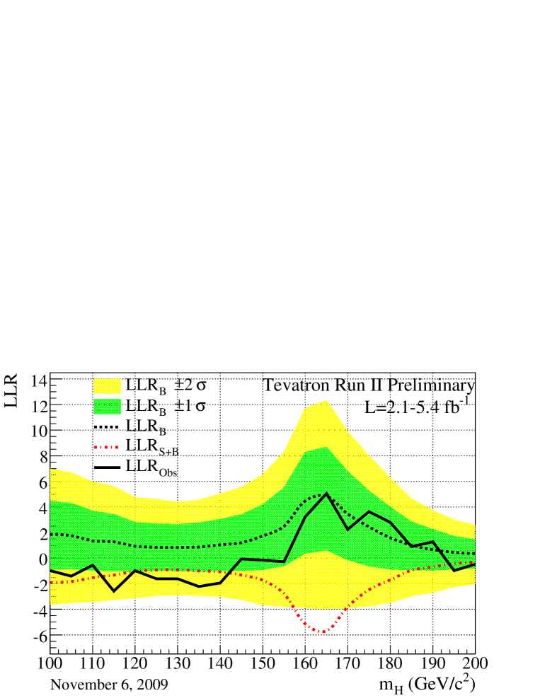
Figure 3: Distributions of the log-likelihood ratio (LLR) as a function of Higgs mass obtained with the $CL_{s}$ method for the combination of all CDF and D0 analyses.

V Combined Results

Before extracting the combined limits we study the distributions of the log-likelihood ratio (LLR) for different hypotheses, to quantify the expected sensitivity across the mass range tested. Figure 3 displays the LLR distributions for the combined analyses as functions of $m_{H}$. Included are the median of the LLR distributions for the background-only hypothesis (LLR_b), the signal-plus-background hypothesis (LLR_s+b), and the observed value for the data (LLR_obs). The shaded bands represent the one and two standard deviation ($\sigma$) departures for LLR_b centered on the median. Table 19 lists the observed and expected LLR values shown in Figure 3.

Table 19: Log-likelihood ratio (LLR) values for the combined CDF + D0 Higgs boson search obtained using the CL_S method.

$m_{H}$ (GeV/$c^{2}$	LLRobs	LLR${}_{S+B}^{\rm{med}}$	LLR${}_{B}^{-2\sigma}$	LLR${}_{B}^{-1\sigma}$	LLR${}_{B}^{\rm{med}}$	LLR${}_{B}^{+1\sigma}$	LLR${}_{B}^{+2\sigma}$
100	-0.99	-1.91	6.99	4.45	1.85	-0.91	-3.63
105	-1.41	-1.83	6.69	4.31	1.75	-0.85	-3.51
110	-0.55	-1.53	5.97	3.69	1.35	-0.99	-3.43
115	-2.58	-1.33	5.61	3.45	1.27	-1.01	-3.25
120	-0.99	-1.01	4.75	2.81	0.93	-1.07	-3.13
125	-1.62	-0.93	4.61	2.69	0.85	-0.99	-2.95
130	-1.61	-0.91	4.37	2.65	0.83	-1.01	-2.89
135	-2.22	-0.99	4.57	2.77	0.87	-1.05	-2.95
140	-1.94	-1.07	5.03	3.05	1.03	-1.03	-3.03
145	-0.07	-1.33	5.55	3.41	1.21	-0.99	-3.25
150	-0.15	-1.73	6.53	4.19	1.73	-0.91	-3.67
155	-0.29	-2.77	8.31	5.51	2.49	-0.61	-3.79
160	3.23	-5.15	11.73	8.29	4.47	0.37	-3.89
165	5.04	-5.69	12.33	8.69	4.85	0.63	-3.97
170	2.24	-3.81	9.91	6.79	3.45	-0.15	-3.91
175	3.64	-2.47	8.01	5.27	2.45	-0.63	-3.75
180	2.79	-1.71	6.27	3.99	1.59	-0.87	-3.49
185	0.90	-0.95	4.65	2.85	1.01	-0.93	-2.97
190	1.28	-0.69	3.73	2.25	0.65	-0.97	-2.69
195	-0.98	-0.43	2.99	1.73	0.45	-0.87	-2.25
200	-0.48	-0.33	2.57	1.47	0.35	-0.81	-2.03

These distributions can be interpreted as follows: The separation between the medians of the LLR_b and LLR_s+b distributions provides a measure of the discriminating power of the search. The sizes of the one- and two-$\sigma$ LLR_b bands indicate the width of the LLR_b distribution, assuming no signal is truly present and only statistical fluctuations and systematic effects are present. The value of LLR_obs relative to LLR_s+b and LLR_b indicates whether the data distribution appears to resemble what we expect if a signal is present (i.e. closer to the LLR_s+b distribution, which is negative by construction) or whether it resembles the background expectation more closely; the significance of any departures of LLR_obs from LLR_b can be evaluated by the width of the LLR_b bands.

Using the combination procedures outlined in Section III, we extract limits on SM Higgs boson production $\sigma\times B(H\rightarrow X)$ in $p\bar{p}$ collisions at $\sqrt{s}=1.96$ TeV for $m_{H}=100-200$ GeV/$c^{2}$. To facilitate comparisons with the standard model and to accommodate analyses with different degrees of sensitivity, we present our results in terms of the ratio of obtained limits to cross section in the SM, as a function of Higgs boson mass, for test masses for which both experiments have performed dedicated searches in different channels. A value of the combined limit ratio which is less than or equal to one indicates that that particular Higgs boson mass is excluded at the 95% C.L.

The combinations of results of each single experiment, as used in this Tevatron combination, yield the following ratios of 95% C.L. observed (expected) limits to the SM cross section: 3.10 (2.38) for CDF and 4.05 (2.80) for D0 at $m_{H}=115$ GeV/$c^{2}$, and 1.18 (1.19) for CDF and 1.53 (1.35) for D0 at $m_{H}=165$ GeV/$c^{2}$.

The ratios of the 95% C.L. expected and observed limit to the SM cross section are shown in Figure 4 for the combined CDF and D0 analyses. The observed and median expected ratios are listed for the tested Higgs boson masses in Table 20 for $m_{H}\leq 150$ GeV/$c^{2}$, and in Table 21 for $m_{H}\geq 155$ GeV/$c^{2}$, as obtained by the Bayesian and the $CL_{S}$ methods. In the following summary we quote the only limits obtained with the Bayesian method, which was decided upon a priori. It turns out that the Bayesian limits are slightly less stringent. The corresponding limits and expected limits obtained using the $CL_{S}$ method are shown alongside the Bayesian limits in the tables. We obtain the observed (expected) values of 2.70 (1.78) at $m_{H}=115$ GeV/$c^{2}$, 1.09 (0.96) at $m_{H}=160$ GeV/$c^{2}$, 0.94 (0.89) at $m_{H}=165$ GeV/$c^{2}$, and 1.29 (1.07) at $m_{H}=170$ GeV/$c^{2}$. This result is obtained with both Bayesian and $CL_{S}$ calculations.

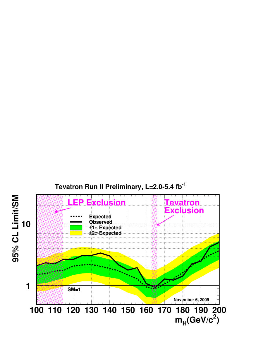
Figure 4: Observed and expected (median, for the background-only hypothesis) 95% C.L. upper limits on the ratios to the SM cross section, as functions of the Higgs boson mass for the combined CDF and D0 analyses. The limits are expressed as a multiple of the SM prediction for test masses (every 5 GeV/$c^{2}$) for which both experiments have performed dedicated searches in different channels. The points are joined by straight lines for better readability. The bands indicate the 68% and 95% probability regions where the limits can fluctuate, in the absence of signal. The limits displayed in this figure are obtained with the Bayesian calculation.

Table 20: Ratios of median expected and observed 95% C.L. limit to the SM cross section for the combined CDF and D0 analyses as a function of the Higgs boson mass in GeV/$c^{2}$, obtained with the Bayesian and with the $CL_{S}$ method.

Bayesian	100	105	110	115	120	125	130	135	140	145	150
Expected	1.52	1.58	1.73	1.78	2.1	2.2	2.2	2.1	1.91	1.75	1.49
Observed	2.11	2.35	2.28	2.70	2.7	3.1	3.1	3.4	3.03	2.17	1.80
$CL_{S}$	100	105	110	115	120	125	130	135	140	145	150
Expected	1.50	1.54	1.64	1.77	2.1	2.2	2.2	2.1	2.0	1.86	1.59
Observed	2.19	2.19	2.16	2.81	2.8	3.2	3.2	3.5	3.2	2.25	2.02

Table 21: Ratios of median expected and observed 95% C.L. limit to the SM cross section for the combined CDF and D0 analyses as a function of the Higgs boson mass in GeV/$c^{2}$, obtained with the Bayesian and with the $CL_{S}$ method.

Bayesian	155	160	165	170	175	180	185	190	195	200
Expected	1.30	0.96	0.89	1.07	1.32	1.63	2.1	2.6	3.2	3.7
Observed	1.96	1.09	0.94	1.29	1.24	1.44	2.3	2.5	4.3	5.0
$CL_{S}$	155	160	165	170	175	180	185	190	195	200
Expected	1.27	0.92	0.89	1.09	1.32	1.64	2.1	2.6	3.2	3.7
Observed	1.74	1.07	0.89	1.21	1.14	1.38	2.1	2.3	4.4	4.8

We also show in Figure 5 and list in Table 22 the observed 1-$CL_{S}$ and its expected distribution for the background-only hypothesis as a functions of the Higgs boson mass, for $m_{H}\geq 150$ GeV/$c^{2}$. This is directly interpreted as the level of exclusion of our search. This figure is obtained using the $CL_{S}$ method. We provide the Log-likelihood ratio (LLR) values for our combined Higgs boson search, as obtained using the $CL_{S}$ method in Figure 3 and Table 19.

In summary, we combine all available CDF and D0 results on SM Higgs search, based on luminosities ranging from 2.1 to 5.4 fb^-1. Compared to our previous combination, more data have been added to the existing channels and analyses have been further optimized to gain sensitivity. We use the latest parton distribution functions and $gg\rightarrow H$ theoretical cross sections when comparing our limits to the SM predictions at high mass.

The 95% C.L. upper limits on Higgs boson production are a factor of 2.70 (0.94) times the SM cross section for a Higgs boson mass of $m_{H}=$115 (165) GeV/$c^{2}$. Based on simulation, the corresponding median expected upper limits are 1.78 (0.89). Standard Model branching ratios, calculated as functions of the Higgs boson mass, are assumed.

We choose to use the intersections of piecewise linear interpolations of our observed and expected rate limits in order to quote ranges of Higgs boson masses that are excluded and that are expected to be excluded. The sensitivities of our searches to Higgs bosons are smooth functions of the Higgs boson mass, and depend most rapidly on the predicted cross sections and the decay branching ratios – the decay $H\rightarrow W^{+}W^{-}$ is the dominant decay for the region of highest sensitivity. The mass resolution of the channels is poor due to the presence of two highly energetic neutrinos in signal events. We therefore use the linear interpolations to extend the results from the 5 GeV/$c^{2}$ mass grid investigated to points in between. This results in higher expected and observed interpolated results than if the full dependence of the cross section and branching ratio were included as well, since the latter produces limit curves that are concave upwards. The region of Higgs boson masses excluded at the 95% C.L. thus obtained is $163<m_{H}<166$ GeV/$c^{2}$. For the first time, the Tevatron combined Higgs searches expect to exclude a SM Higgs boson for specific masses, assuming no Higgs boson production. The mass range expected to be excluded is $159<m_{H}<168$ GeV/$c^{2}$. The excluded region obtained by finding the intersections of the linear interpolations of the observed $1-CL_{S}$ curve shown in Figure 5 is larger than that obtained with the Bayesian calculation. We choose to quote the exclusion region using the Bayesian calculation.

While new data have been added and the sensitivity of the analyses has thus increased, the observed exclusion region is slightly smaller than to that obtained in March 2009 prevhiggs , which excluded the range $160<m_{H}<170$ GeV/$c^{2}$. The new data added have excess signal-like candidates relative to the background predictions in the high-mass $H\rightarrow W^{+}W^{-}$ channels, but the total excess in the new data is less than one standard deviation in size.

The results presented in this paper significantly extend the individual limits of each collaboration and our previous combination. The sensitivity of our combined search is sufficient to exclude a Higgs boson at high mass and is expected to grow substantially in the near future with the additional luminosity already recorded at the Tevatron and not yet analyzed, and with additional improvements of our analysis techniques which will be propagated in the current and future analyses.

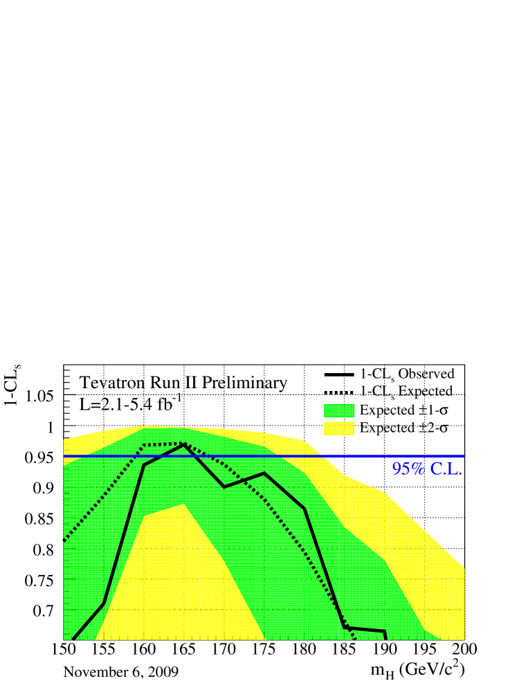
Figure 5: The exclusion strength 1-$CL_{S}$ as a function of the Higgs boson mass (in steps of 5 GeV/$c^{2}$), as obtained with $CL_{S}$ method. for the combination of the CDF and D0 analyses.

Table 22: The observed and expected CL_s values as functions of $m_{H}$, for the combined CDF and D0 Higgs boson searches.

$m_{H}$ (GeV/$c^{2}$)	CL${}_{\rm s}^{\rm{obs}}$	CL${}_{\rm s}^{-2\sigma}$	CL${}_{\rm s}^{-1\sigma}$	CL${}_{\rm s}^{\rm{median}}$	CL${}_{\rm s}^{+1\sigma}$	CL${}_{\rm s}^{+2\sigma}$
100	0.562	0.968	0.931	0.829	0.571	0.258
105	0.500	0.968	0.940	0.809	0.565	0.255
110	0.563	0.948	0.914	0.765	0.506	0.212
115	0.268	0.963	0.897	0.735	0.470	0.200
120	0.401	0.945	0.850	0.673	0.389	0.138
125	0.300	0.894	0.815	0.646	0.391	0.137
130	0.288	0.901	0.833	0.639	0.378	0.135
135	0.217	0.922	0.842	0.649	0.389	0.143
140	0.283	0.915	0.862	0.693	0.412	0.158
145	0.591	0.943	0.881	0.727	0.473	0.185
150	0.633	0.977	0.934	0.812	0.545	0.232
155	0.710	0.991	0.964	0.886	0.682	0.370
160	0.936	1.000	0.995	0.968	0.853	0.590
165	0.969	0.997	0.996	0.971	0.873	0.623
170	0.900	0.994	0.981	0.937	0.780	0.478
175	0.922	0.988	0.965	0.880	0.657	0.338
180	0.865	0.975	0.923	0.794	0.550	0.237
185	0.671	0.918	0.834	0.682	0.407	0.145
190	0.665	0.890	0.780	0.571	0.324	0.100
195	0.235	0.828	0.667	0.489	0.252	0.070
200	0.272	0.766	0.629	0.439	0.219	0.059

References

- (1) CDF Collaboration, “Combined Upper Limit on Standard Model Higgs Boson Production for HCP 2009”, CDF Conference Note 9999 (2009).
- (2) “Combined Upper Limits on Standard Model Higgs Boson Production from the D0 Experiment in 2.1-5.4 fb-1”, D0 Conference Note 6008 (2009).
-
(3)
CDF Collaboration, “Combined Upper Limit on
Standard Model Higgs Boson Production for Summer 2009”, CDF Conference Note 9807 (2009);
D0 Collaboration, “Combined upper limits on Standard Model Higgs boson production from the D0 experiment in 0.9-5.0 fb-1”, D0 Conference Note 5984 (2009);
CDF Collaboration, “Combined Upper Limit on Standard Model Higgs Boson Production for Winter 2009”, CDF Conference Note 9674 (2009);
D0 Collaboration, “Combined upper limits on standard model Higgs boson production from the D0 experiment with up to 4.2 fb-1 of data” D0 Conference Note 5896 (2009);
The CDF and D0 Collaborations and the TEVNPHWG Working Group, “Combined CDF and DZero Upper Limits on Standard Model Higgs-Boson Production with up to 4.2 fb-1 of Data”, FERMILAB-PUB-09-060-E, CDF Note 9713, D0 Note 5889, arXiv:0903.4001v1 [hep-ex] (2009). - (4) CDF Collaboration, “Search for Higgs Boson Production in Association with a Boson with 4.3 fb-1 with Neural Networks”, CDF Conference Note 9997 (2009).
- (5) CDF Collaboration, “Search for Standard Model Higgs Boson Production in Association With a Boson Using Matrix Element Techniques with 4.3 fb-1 of CDF Data”, CDF Conference Note 9985 (2009).
- (6) CDF Collaboration, “Search for the Standard Model Higgs Boson in the Plus Jets Sample”, CDF Conference Note 9642 (2009).
- (7) CDF Collaboration, “A Search for the Standard Model Higgs boson in the Process Using 4.1 fb-1 of CDF II Data”, CDF Conference Note 9889 (2009).
- (8) CDF Collaboration, “Search for Production Using 4.8 fb-1 of Data”, CDF Conference Note 9887 (2009).
- (9) CDF Collaboration, “Search for SM Higgs using tau leptons using 2 fb-1”, CDF Conference Note 9179.
- (10) CDF Collaboration, “A Search for the Standard Model Higgs Boson in the All-Hadronic channel using a Matrix Element Method”, CDF Conference Note 9366.
- (11) D0 Collaboration, “Search for WH associated production using neural networks with 5.0 fb-1 of Tevatron data,” D0 Conference Note 5972.
- (12) D0 Collaboration, “Search for the standard model Higgs boson in final states”, D0 Conference note 5844.
- (13) D0 Collaboration, “Search for the standard model Higgs boson in the final state”, D0 Conference note 5845.
- (14) D0 Collaboration, “Search for the standard model Higgs boson in the channel in 5.2 fb-1 of collisions at TeV”, D0 Conference note 5872.
- (15) D0 Collaboration, “A Search for and Production in 4.2 fb-1 of data with the D0 detector in Collisions at TeV”, D0 Conference Note 5876.
- (16) D0 Collaboration, “Search for associated Higgs boson production in collisions at TeV”, D0 Conference Note 5485.
- (17) D0 Collaboration, “Search for associated Higgs boson production with like sign leptons in collisions at TeV”, D0 Conference Note 5873.
- (18) D0 Collaboration, “Search for Higgs production in dilepton plus missing transverse energy final states with 5.4 fb-1 of collisions at TeV”, D0 Conference Note 6006.
- (19) D0 Collaboration, “Search for the Standard Model Higgs boson in final states at D0 with 4.2 fb-1 of data”, D0 Conference Note 5858.
- (20) D0 Collaboration, “Search for the standard model Higgs boson in the channel”, D0 Conference note 5739.
- (21) C. Anastasiou, G. Dissertori, M. Grazzini, F. Stöckli and B. R. Webber, JHEP 0908, 099 (2009) [arXiv:0905.3529 [hep-ph]].
- (22) T. Sjöstrand, L. Lonnblad and S. Mrenna, “PYTHIA 6.2: Physics and manual,” arXiv:hep-ph/0108264.
- (23) H. L. Lai et al., “Improved Parton Distributions from Global Analysis of Recent Deep Inelastic Scattering and Inclusive Jet Data”, Phys. Rev D 55, 1280 (1997).
- (24) C. Anastasiou, R. Boughezal and F. Petriello, “Mixed QCD-electroweak corrections to Higgs boson production in gluon fusion”, arXiv:0811.3458 [hep-ph] (2008).
- (25) D. de Florian and M. Grazzini, “Higgs production through gluon fusion: updated cross sections at the Tevatron and the LHC”, arXiv:0901.2427v1 [hep-ph] (2009).
- (26) The CDF and D0 Collaborations and the TEVNPHWG Working Group, “Combined CDF and D0 Upper Limits on Standard Model Higgs Boson Production at Higg Mass (155-200 GeV) with 3 fb-1 of Data”, FERMILAB-PUB-08-270-E, CDF Note 9465, D0 Note 5754, arXiv:0808.0534v1 [hep-ex] (2008).
- (27) S. Catani, D. de Florian, M. Grazzini and P. Nason, “Soft-gluon resummation for Higgs boson production at hadron colliders,” JHEP 0307, 028 (2003) [arXiv:hep-ph/0306211].
- (28) K. A. Assamagan et al. [Higgs Working Group Collaboration], “The Higgs working group: Summary report 2003,” arXiv:hep-ph/0406152.
- (29) U. Aglietti, R. Bonciani, G. Degrassi, A. Vicini, “Two-loop electroweak corrections to Higgs production in proton-proton collisions”, arXiv:hep-ph/0610033v1 (2006).
- (30) A. D. Martin, W. J. Stirling, R. S. Thorne and G. Watt, “Parton distributions for the LHC”, arXiv:0901.0002 [hep-ph] (2009).
- (31) A. D. Martin, R. G. Roberts, W. J. Stirling and R. S. Thorne, Phys. Lett. B 531, 216 (2002) [arXiv:hep-ph/0201127].
- (32) O. Brein, A. Djouadi, and R. Harlander, “NNLO QCD corrections to the Higgs-strahlung processes at hadron colliders”, Phys. Lett. B579, 2004, 149-156.
- (33) Ciccolini, M. L. and Dittmaier, S. and Kramer, M., “Electroweak radiative corrections to associated W H and Z H production at hadron colliders”, Phys. Rev. D68 (2003) 073003.
- (34) E. Berger and J. Campbell. “Higgs boson production in weak boson fusion at next-to-leading order”, Phys. Rev. D70 (2004) 073011,
- (35) A. Djouadi, J. Kalinowski and M. Spira, “HDECAY: A program for Higgs boson decays in the standard model and its supersymmetric extension,” Comput. Phys. Commun. 108, 56 (1998) [arXiv:hep-ph/9704448].
- (36) M. L. Mangano, M. Moretti, F. Piccinini, R. Pittau and A. D. Polosa, “ALPGEN, a generator for hard multiparton processes in hadronic collisions,” JHEP 0307, 001 (2003) [arXiv:hep-ph/0206293].
- (37) S. Frixione and B.R. Webber, JHEP 06, 029 (2002) [arXiv:hep-ph/0204244]
- (38) G. Corcella et al., “HERWIG 6: An event generator for hadron emission reactions with interfering gluons (including supersymmetric processes),” JHEP 0101, 010 (2001) [arXiv:hep-ph/0011363].
- (39) A. Pukhov et al., “CompHEP: A package for evaluation of Feynman diagrams and integration over multi-particle phase space. User’s manual for version 33,” [arXiv:hep-ph/9908288].
- (40) T. Junk, Nucl. Instrum. Meth. A434, p. 435-443, 1999, A.L. Read, “Modified frequentist analysis of search results (the method)”, in F. James, L. Lyons and Y. Perrin (eds.), Workshop on Confidence Limits, CERN, Yellow Report 2000-005, available through cdsweb.cern.ch.
- (41) W. Fisher, “Systematics and Limit Calculations,” FERMILAB-TM-2386-E.
- (42) S. Moch and P. Uwer, Nucl. Phys. Proc. Suppl. 183, 75 (2008) [arXiv:0807.2794 [hep-ph]].
- (43) The CDF and D0 Collaborations and the Tevatron Electroweak Working Group, arXiv:0808.1089 [hep-ex].
- (44) A. D. Martin, W. J. Stirling, R. S. Thorne and G. Watt, Phys. Lett. B 652, 292 (2007) [arXiv:0706.0459 [hep-ph]].
-
(45)
M. Cacciari, S. Frixione, M. L. Mangano, P. Nason and G. Ridolfi,
JHEP 0809, 127 (2008)
[arXiv:0804.2800 [hep-ph]];
N. Kidonakis and R. Vogt, Phys. Rev. D 78, 074005 (2008) [arXiv:0805.3844 [hep-ph]]. - (46) N. Kidonakis, Phys. Rev. D 74, 114012 (2006) [arXiv:hep-ph/0609287].
- (47) B. W. Harris, E. Laenen, L. Phaf, Z. Sullivan and S. Weinzierl, Phys. Rev. D 66, 054024 (2002) [arXiv:hep-ph/0207055].
- (48) J. Campbell and R. K. Ellis, http://mcfm.fnal.gov/.