Phase transitions and metastability in the distribution of the bipartite entanglement of a large quantum system

A. De Pasquale Dipartimento di Fisica, Università di Bari, I-70126 Bari, Italy INFN, Sezione di Bari, I-70126 Bari, Italy MECENAS, Università Federico II di Napoli, Via Mezzocannone 8, I-80134 Napoli, Italy    P. Facchi INFN, Sezione di Bari, I-70126 Bari, Italy Dipartimento di Matematica, Università di Bari, I-70125 Bari, Italy    G. Parisi Dipartimento di Fisica, Università di Roma “La Sapienza”, Piazzale Aldo Moro 2, 00185 Roma, Italy Centre for Statistical Mechanics and Complexity (SMC), CNR-INFM, 00185 Roma, Italy
INFN, Sezione di Roma, 00185 Roma, Italy
   S. Pascazio Dipartimento di Fisica, Università di Bari, I-70126 Bari, Italy INFN, Sezione di Bari, I-70126 Bari, Italy    A. Scardicchio Abdus Salam International Center for Theoretical Physics, Strada Costiera 11, I-34014 Trieste, Italy INFN, Sezione di Trieste, I-34014 Trieste, Italy
Abstract

We study the distribution of the Schmidt coefficients of the reduced density matrix of a quantum system in a pure state. By applying general methods of statistical mechanics, we introduce a fictitious temperature and a partition function and translate the problem in terms of the distribution of the eigenvalues of random matrices. We investigate the appearance of two phase transitions, one at a positive temperature, associated to very entangled states, and one at a negative temperature, signalling the appearance of a significant factorization in the many-body wave function. We also focus on the presence of metastable states (related to 2-D quantum gravity) and study the finite size corrections to the saddle point solution.

pacs:
03.67.Mn, 03.65.Ud, 68.35.Rh

I Introduction

Entanglement is an important resource in quantum information processing and quantum enabled technologies nielsen ; benenticasati . Besides its important applications in relatively simple systems, that can be described in terms of a few effective quantum variables, it is also widely investigated in many-body systems Amico08 ; h4 , where the bipartite entanglement can be given a satisfactory quantitative definition in terms of entropy and its linearized versions, such as purity woot ; entanglement2 . The characterization of the global features of entanglement is more involved, unveiling in general different features of the many-body wave function multipart ; mmes , and it is becoming clear that the multipartite entanglement of a large system cannot be fully characterized in terms of a single (or a few) measure(s).

Entanglement measures the nonclassical correlations between the different components of a quantum system and unearths different characteristics of its many-body wave-function. When the quantum system is large, it becomes therefore interesting to scrutinize the features of the distribution of some bipartite entanglement measure, such as the purity or the Von Neumann entropy. Besides being of interest for applications, this is an interesting problem in statistical mechanics. In paper1 we tackled this problem by studying a random matrix model that describes the statistical properties of the eigenvalues of the reduced density matrix of a subsystem A𝐴A of dimension N𝑁N (the complementary subsystem B𝐵B having the same dimension as A𝐴A). In the limit of large system dimension N𝑁N, we introduced a partition function for the canonical ensemble as a function of a fictitious temperature. The role of energy is played by purity: different temperatures correspond to different entanglement. The most important result of our analysis was the proof that the different regions of entanglement, corresponding to different ranges of the fictitious temperature, are separated by phase transitions.

One puzzle was left open in that paper: in the region of negative temperatures our solution suddenly ceased to exist at a critical βgsubscript𝛽𝑔\beta_{g} where the average purity of subsytem A𝐴A was πAB=9/4Nsubscript𝜋𝐴𝐵94𝑁\pi_{AB}=9/4N (a phenomenon quite common in random matrix theory, as this critical point corresponds to tesselations of random surfaces, or 2-D quantum gravity). As the partition function exists for all β𝛽\beta\in\mathbb{R}, the region of factorizable states, where πAB=𝒪(1)subscript𝜋𝐴𝐵𝒪1\pi_{AB}={\cal O}\left(1\right), was not covered.

We will show in this paper that the solution in paper1 becomes metastable for any β<0𝛽0\beta<0 (in the scaling of paper1 ) and a new stable solution appears which interpolates smoothly from πAB=2/Nsubscript𝜋𝐴𝐵2𝑁\pi_{AB}=2/N to πAB=1subscript𝜋𝐴𝐵1\pi_{AB}=1 as β𝛽\beta goes from 00 to -\infty. Moreover, we will also study the metastable solution that is born at β=0𝛽0\beta=0 and follow it through the region 0>β>0𝛽0>\beta>-\infty.

This paper is organized as follows. In Sec. II we introduce the notation and set the bases of the statistical mechanical approach to the problem. In Sec. III we study positive temperatures, where at very low temperatures we find very entangled states. Negative temperatures are investigated in Sec. IV, where it is shown that two branches exist, a stable one associated to a partial factorization of the many-body wave function, and a metastable one which contains the 2D-quantum gravity point. The finite size corrections are investigated in Sec. V. We discuss the implications of our results for quantum information in Sec. VI and we conclude in Sec. VII by summarizing our findings and discussing them in terms of future perspectives.

II A statistical approach to the study of bipartite entanglement

We start off by describing a statistical approach to the study of bipartite entanglement for large quantum systems. We will tackle this problem by introducing a partition function paper1 .

Consider a bipartite system, composed of two subsystems A𝐴A and B𝐵B. The total system lives in the tensor product Hilbert space =ABtensor-productsubscript𝐴subscript𝐵\mathcal{H}=\mathcal{H}_{A}\otimes\mathcal{H}_{B}, with dimA=NdimB=Mdimensionsubscript𝐴𝑁dimensionsubscript𝐵𝑀\dim\mathcal{H}_{A}=N\leq\dim\mathcal{H}_{B}=M. We assume that the system is in a pure state |ψ>ket𝜓|\psi\big{>}\in\mathcal{H}. The reduced density matrix of subsystem A𝐴A reads

ρA=TrB|ψ><ψ|subscript𝜌𝐴subscriptTr𝐵ket𝜓bra𝜓\rho_{A}={\rm Tr}_{B}|\psi\big{>}\big{<}\psi| (1)

and is a Hermitian, positive, unit-trace N×N𝑁𝑁N\times N matrix. A good measure of the entanglement between the two subsystems is given by the purity

πAB=TrAρA2=TrBρB2=j=1Nλj2[1/N,1],subscript𝜋𝐴𝐵subscriptTr𝐴superscriptsubscript𝜌𝐴2subscriptTr𝐵superscriptsubscript𝜌𝐵2superscriptsubscript𝑗1𝑁superscriptsubscript𝜆𝑗21𝑁1\pi_{AB}={\rm Tr}_{A}\rho_{A}^{2}={\rm Tr}_{B}\rho_{B}^{2}=\sum_{j=1}^{N}\lambda_{j}^{2}\in[1/N,1], (2)

whose minimum is attained when all the eigenvalues λjsubscript𝜆𝑗\lambda_{j} are equal to 1/N1𝑁1/N (completely mixed state and maximal entanglement between the two bipartitions), while its maximum (attained when one eigenvalue is 1 and all others are 0) detects a factorized state (no entanglement).

In order to study the statistics of bipartite entanglement for pure quantum states, we consider typical vector states |ψ>ket𝜓|\psi\big{>} aaa ; page , sampled according to the unique, unitarily invariant measure. The significance of this measure can be understood in the following way: consider a reference state vector |ψ0>ketsubscript𝜓0|\psi_{0}\big{>} and a unitary transformation |ψ>=U|ψ0>ket𝜓𝑈ketsubscript𝜓0|\psi\big{>}=U|\psi_{0}\big{>}. In the least set of assumptions on U𝑈U, the measure is chosen in a unique way, being the only left- and right-invariant Haar (probability) measure of the unitary group U(N2)𝑈superscript𝑁2U(N^{2}). The final state |ψ>ket𝜓|\psi\big{>} will hence be distributed according to the measure mentioned above (independently of |ψ0>ketsubscript𝜓0|\psi_{0}\big{>}). Notice the analogy with the maximum entropy argument in classical statistical mechanics. By tracing over subsystem B𝐵B, this measure induces the following measure over the space of Hermitian, positive matrices of unit trace aaa ; page

dμ(ρA)𝑑𝜇subscript𝜌𝐴\displaystyle d\mu(\rho_{A}) =\displaystyle= 𝒟ρA(detρA)MNδ(1TrρA),𝒟subscript𝜌𝐴superscriptsubscript𝜌𝐴𝑀𝑁𝛿1Trsubscript𝜌𝐴\displaystyle{\cal D}\rho_{A}(\det\rho_{A})^{M-N}\delta(1-{\rm Tr}\rho_{A}), (3)
=\displaystyle= dNλi<j(λiλj)2ληNδ(1kλk),superscript𝑑𝑁𝜆subscriptproduct𝑖𝑗superscriptsubscript𝜆𝑖subscript𝜆𝑗2subscriptproductsuperscriptsubscript𝜆𝜂𝑁𝛿1subscript𝑘subscript𝜆𝑘\displaystyle d^{N}\lambda\prod_{i<j}(\lambda_{i}-\lambda_{j})^{2}\prod_{\ell}\lambda_{\ell}^{\eta N}\delta\left(1-\sum_{k}\lambda_{k}\right),

where λksubscript𝜆𝑘\lambda_{k} are the (positive) eigenvalues of ρAsubscript𝜌𝐴\rho_{A} (Schmidt coefficients), we dropped the volume of the U(N)𝑈𝑁U(N) group (which is irrelevant for our purposes) and ηNMN𝜂𝑁𝑀𝑁\eta N\equiv M-N is the difference between the dimensions of the Hilbert spaces Asubscript𝐴\mathcal{H}_{A} and Bsubscript𝐵\mathcal{H}_{B}. In order to study the statistical behavior of a large bipartite quantum system we introduce a partition function from which all the thermodynamic quantities, for example the entropy or the free energy, can be computed:

𝒵AB=𝑑μ(ρA)exp(βNαπAB),subscript𝒵𝐴𝐵differential-d𝜇subscript𝜌𝐴𝛽superscript𝑁𝛼subscript𝜋𝐴𝐵{\cal Z}_{AB}=\int d\mu(\rho_{A})\exp\left(-\beta N^{\alpha}\pi_{AB}\right), (4)

where α𝛼\alpha is a positive integer (either 2 or 3, as we shall see) and β𝛽\beta a fictitious temperature “selecting” different regions of entanglement. The value of α𝛼\alpha needs to be chosen in order to yield the correct thermodynamic limit as

NαπAB=𝒪(N2),superscript𝑁𝛼delimited-⟨⟩subscript𝜋𝐴𝐵𝒪superscript𝑁2N^{\alpha}\langle\pi_{AB}\rangle={\cal O}\left(N^{2}\right), (5)

since N2superscript𝑁2N^{2} is the number of degrees of freedom of the matrix ρAsubscript𝜌𝐴\rho_{A}. Around the maximally entangled states (for β>0𝛽0\beta>0 paper1 ) we have πAB=𝒪(1/N)delimited-⟨⟩subscript𝜋𝐴𝐵𝒪1𝑁\langle\pi_{AB}\rangle={\cal O}\left(1/N\right) so α=3𝛼3\alpha=3, while around separable states (for β<0𝛽0\beta<0) we have πAB=𝒪(1)delimited-⟨⟩subscript𝜋𝐴𝐵𝒪1\langle\pi_{AB}\rangle={\cal O}\left(1\right) and hence α=2𝛼2\alpha=2. In the following we will assume η=0𝜂0\eta=0, since this does not change the qualitative picture (the extension to η0𝜂0\eta\neq 0 being straightforward but computationally cumbersome).

Since the purity depends only on the eigenvalues of ρAsubscript𝜌𝐴\rho_{A} the partition function reads

𝒵AB=λi0dNλi<j(λiλj)2δ(1i=1Nλi)eβNαiλi2,subscript𝒵𝐴𝐵subscriptsubscript𝜆𝑖0superscript𝑑𝑁𝜆subscriptproduct𝑖𝑗superscriptsubscript𝜆𝑖subscript𝜆𝑗2𝛿1superscriptsubscript𝑖1𝑁subscript𝜆𝑖superscript𝑒𝛽superscript𝑁𝛼subscript𝑖superscriptsubscript𝜆𝑖2{\cal Z}_{AB}=\int_{\lambda_{i}\geq 0}d^{N}\lambda\prod_{i<j}(\lambda_{i}-\lambda_{j})^{2}\delta\left(1-\sum_{i=1}^{N}\lambda_{i}\right)e^{-\beta N^{\alpha}\sum_{i}\lambda_{i}^{2}}, (6)

which by introducing a Lagrange multiplier for the delta function yields

𝒵ABsubscript𝒵𝐴𝐵\displaystyle{\cal Z}_{AB} =\displaystyle= N2dξ2πλi0dNλsuperscript𝑁2superscriptsubscript𝑑𝜉2𝜋subscriptsubscript𝜆𝑖0superscript𝑑𝑁𝜆\displaystyle N^{2}\int_{-\infty}^{\infty}\frac{d\xi}{2\pi}\int_{\lambda_{i}\geq 0}d^{N}\lambda (7)
×eiN2ξ(1iλi)βNαiλi2+2i<jln|λiλj|.absentsuperscript𝑒𝑖superscript𝑁2𝜉1subscript𝑖subscript𝜆𝑖𝛽superscript𝑁𝛼subscript𝑖superscriptsubscript𝜆𝑖22subscript𝑖𝑗subscript𝜆𝑖subscript𝜆𝑗\displaystyle\times e^{iN^{2}\xi(1-\sum_{i}\lambda_{i})-\beta N^{\alpha}\sum_{i}\lambda_{i}^{2}+2\sum_{i<j}\ln|\lambda_{i}-\lambda_{j}|}.\;

A physical interpretation of the exponent in the integrand of the partition function can be given as follows mehta : the eigenvalues of ρAsubscript𝜌𝐴\rho_{A} can be interpreted as a gas of interacting point charges (Coulomb gas) at positions λisubscript𝜆𝑖\lambda_{i}’s, on the positive half-line and with a quadratic potential. The solution of these integrals is known (as Selberg’s integral) for the case in which the integration limits are <λi<+subscript𝜆𝑖-\infty<\lambda_{i}<+\infty mehta .

The constraint of the positivity of the eigenvalues makes the computation of this integral far more complicated. Although a exact solution for finite N𝑁N is unlikely to be found 111An exact solution can always be found by means of the orthogonal polynomials method, but the expressions for 𝒵ABsubscript𝒵𝐴𝐵{\cal Z}_{AB} grow enormously in complexity with increasing N𝑁N. (but see Giraud ; paper1 for the first few moments), the problem arising from the constraint on the positivity of the eigenvalues can be overcome in the large N𝑁N limit, as we will look for the stationary point of the exponent with respect to both the λ𝜆\lambda’s and ξ𝜉\xi. In particular, the contour of integration for ξ𝜉\xi lies on the real axis, but we will soon see that the saddle point for ξ𝜉\xi lies on the imaginary ξ𝜉\xi axis. It is then understood that the contour needs to be deformed to pass by this point parallel to the line of steepest descent. For the saddle point we need to find the minimum of the free energy:

βF=βNαiλi22i<jln|λiλj|iN2ξ(1iλi).𝛽𝐹𝛽superscript𝑁𝛼subscript𝑖superscriptsubscript𝜆𝑖22subscript𝑖𝑗subscript𝜆𝑖subscript𝜆𝑗𝑖superscript𝑁2𝜉1subscript𝑖subscript𝜆𝑖\beta F=\beta N^{\alpha}\sum_{i}\lambda_{i}^{2}-2\sum_{i<j}\ln|\lambda_{i}-\lambda_{j}|-iN^{2}\xi\left(1-\sum_{i}\lambda_{i}\right). (8)

By varying F𝐹F we find the saddle point equations

2βNαλi+2ji1λiλjiN2ξ2𝛽superscript𝑁𝛼subscript𝜆𝑖2subscript𝑗𝑖1subscript𝜆𝑖subscript𝜆𝑗𝑖superscript𝑁2𝜉\displaystyle-2\beta N^{\alpha}\lambda_{i}+2\sum_{j\neq i}\frac{1}{\lambda_{i}-\lambda_{j}}-iN^{2}\xi =\displaystyle= 0,0\displaystyle 0, (9)
iλisubscript𝑖subscript𝜆𝑖\displaystyle\sum_{i}\lambda_{i} =\displaystyle= 1.1\displaystyle 1. (10)

In the following sections we will separately analyze the range of positive and negative temperatures, and unveil the presence of two phase transitions for the system, a second order one at a positive critical β𝛽\beta and a first order one at a negative critical β𝛽\beta.

II.1 The global picture

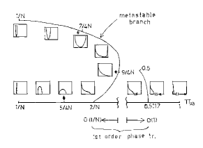
Before proceeding to a formal analysis of the phase transitions, it is convenient to give a qualitative picture of the behavior of the Schmidt coefficients as the temperature is changed. As the inverse temperature is decreased, the density matrix of subsystem A𝐴A changes as follows. As β+𝛽\beta\to+\infty all eigenvalues are =1/Nabsent1𝑁=1/N (maximally mixed state). As β𝛽\beta decreases, we encounter two phase transitions: one at a positive critical value β+subscript𝛽\beta_{+} and one at a negative critical value βsubscript𝛽\beta_{-}, both critical values being to be determined. For β>β+𝛽subscript𝛽\beta>\beta_{+} all eigenvalues remain 𝒪(1/N)𝒪1𝑁{\cal O}\left(1/N\right), their distribution being characterized, as we shall see, by the Wigner semicircle law. After the first phase transition, for β+>β>βsubscript𝛽𝛽subscript𝛽\beta_{+}>\beta>\beta_{-}, the eigenvalues, all always 𝒪(1/N)𝒪1𝑁{\cal O}\left(1/N\right), follow the Wishart distribution, divergent at the origin. Finally, after the second phase transition, for β<β𝛽subscript𝛽\beta<\beta_{-}, one eigenvalue becomes 𝒪(1)𝒪1{\cal O}\left(1\right), “evaporating” from the “sea” of eigenvalues 𝒪(1/N)𝒪1𝑁{\cal O}\left(1/N\right): this is a signature of the emergence of factorization in the many-body wave function, the eigenvalue 𝒪(1)𝒪1{\cal O}\left(1\right) being associated with a significant separability between subsystems A𝐴A and B𝐵B. For β𝛽\beta\to-\infty the many body wavefunction is fully factorized. Pictorially, the typical eigenvalues vector evolves starting from β=+𝛽\beta=+\infty to β=𝛽\beta=-\infty as

(1N,1N,,1N)β+subscript1𝑁1𝑁1𝑁𝛽\displaystyle\underbrace{\left(\frac{1}{N},\frac{1}{N},...,\frac{1}{N}\right)}_{\beta\to+\infty} \displaystyle\longrightarrow (𝒪(1N),,𝒪(1N))+>β>β+subscript𝒪1𝑁𝒪1𝑁𝛽subscript𝛽\displaystyle\underbrace{\left({\cal O}\left(\frac{1}{N}\right),...,{\cal O}\left(\frac{1}{N}\right)\right)}_{+\infty>\beta>\beta_{+}} (11)
\displaystyle\longrightarrow (𝒪(1N),𝒪(1N),,0,,0)β+>β>βsubscript𝒪1𝑁𝒪1𝑁00subscript𝛽𝛽subscript𝛽\displaystyle\underbrace{\left({\cal O}\left(\frac{1}{N}\right),{\cal O}\left(\frac{1}{N}\right),...,0,...,0\right)}_{\beta_{+}>\beta>\beta_{-}}
\displaystyle\longrightarrow (𝒪(1),𝒪(1N),,0,,0)β>β>subscript𝒪1𝒪1𝑁00subscript𝛽𝛽\displaystyle\underbrace{\left({\cal O}\left(1\right),{\cal O}\left(\frac{1}{N}\right),...,0,...,0\right)}_{\beta_{-}>\beta>-\infty}
\displaystyle\longrightarrow (1,0,,0)β,subscript100𝛽\displaystyle\underbrace{\left(1,0,...,0\right)}_{\beta\to-\infty},

where the zeroes in the second and third lines mean an accumulation of points around the origin, and we will find that [in the scaling of β𝛽\beta given by α=3𝛼3\alpha=3 in Eq. (5)], β+=2subscript𝛽2\beta_{+}=2 and β=2.455/Nsubscript𝛽2.455𝑁\beta_{-}=-2.455/N.

III Positive temperatures: towards maximally entangled states

In this section we will consider the range of positive temperatures: 0<β<+0𝛽0<\beta<+\infty; in particular we will study the occurrence of a second order phase transition at β=2𝛽2\beta=2 paper1 . We will use a novel more general method, that will enable us to find all solutions and can be easily extended to negative temperatures.

From the expression of the partition function one can easily infer that when β+𝛽\beta\rightarrow+\infty the typical states belonging to this distribution are maximally entangled states and correspond to the case λi=1/Nsubscript𝜆𝑖1𝑁\lambda_{i}=1/N, i{1,N}for-all𝑖1𝑁\forall i\in\{1,\ldots N\}. It then follows that for this range of temperatures the right scaling exponent in (4)-(5) is α=3𝛼3\alpha=3.

In order to estimate the thermodynamic quantities of the system we solve the saddle point equations (9)-(10) in the continuous limit, by introducing the natural scaling

λi=1Nλ(ti),0<ti=iN1.formulae-sequencesubscript𝜆𝑖1𝑁𝜆subscript𝑡𝑖0subscript𝑡𝑖𝑖𝑁1\lambda_{i}=\frac{1}{N}\lambda(t_{i}),\qquad 0<t_{i}=\frac{i}{N}\leq 1. (12)

In the limit N𝑁N\to\infty, Eq. (9) becomes

βλ+P0𝑑λρ(λ)λλiξ2=0,𝛽𝜆𝑃superscriptsubscript0differential-dsuperscript𝜆𝜌superscript𝜆𝜆superscript𝜆𝑖𝜉20-\beta\lambda+P\int_{0}^{\infty}d\lambda^{\prime}\frac{\rho(\lambda^{\prime})}{\lambda-\lambda^{\prime}}-i\frac{\xi}{2}=0, (13)

which is a singular Fredholm equation of the first kind, known as Tricomi equation tricomi . The function

ρ(λ)=01𝑑tδ(λλ(t))𝜌𝜆superscriptsubscript01differential-d𝑡𝛿𝜆𝜆𝑡\rho(\lambda)=\int_{0}^{1}dt\;\delta(\lambda-\lambda(t)) (14)

is the density of eigenvalues we want to determine. A similar equation, restricted at β=0𝛽0\beta=0, was studied by Page page .

Refer to caption
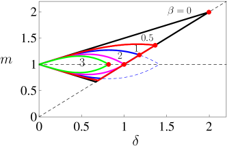
Figure 1: Solution domain for different values of temperature: for each value of β𝛽\beta (indicated) the relative full line encloses the region of the parameter space such that the eigenvalue density is positive. The line m=δ𝑚𝛿m=\delta corresponds to the positive eigenvalues condition.

According to the Tricomi theorem tricomi ; page the solution of the integral equation (13) lies in a compact interval [a,b]𝑎𝑏[a,b], (0ab0𝑎𝑏0\leq a\leq b). Let us set

m=a+b2,δ=ba2,0δm.formulae-sequence𝑚𝑎𝑏2formulae-sequence𝛿𝑏𝑎20𝛿𝑚m=\frac{a+b}{2},\qquad\delta=\frac{b-a}{2},\qquad 0\leq\delta\leq m. (15)

We map the interval [a,b]𝑎𝑏[a,b] into the interval [1,1]11[-1,1] by introducing the following change of variables:

λ=m+xδ,ϕ(x)=ρ(λ)δ.formulae-sequence𝜆𝑚𝑥𝛿italic-ϕ𝑥𝜌𝜆𝛿\lambda=m+x\delta,\qquad\phi(x)=\rho(\lambda)\delta. (16)

We get

1πP11ϕ(y)yx𝑑y=g(x),1𝜋𝑃superscriptsubscript11italic-ϕ𝑦𝑦𝑥differential-d𝑦𝑔𝑥\frac{1}{\pi}P\int_{-1}^{1}\frac{\phi(y)}{y-x}dy=g(x), (17)

with

g(x)=1π(iξδ2+βδm+βδ2x),𝑔𝑥1𝜋𝑖𝜉𝛿2𝛽𝛿𝑚𝛽superscript𝛿2𝑥g(x)=-\frac{1}{\pi}\left(i\xi\frac{\delta}{2}+\beta\delta m+\beta\delta^{2}x\right), (18)

whose normalized solution (ϕ𝑑x=1italic-ϕdifferential-d𝑥1\int\phi\,dx=1) is

ϕ(x)=1πP111y21x2g(y)yx𝑑y+1π1x2,italic-ϕ𝑥1𝜋𝑃superscriptsubscript111superscript𝑦21superscript𝑥2𝑔𝑦𝑦𝑥differential-d𝑦1𝜋1superscript𝑥2\phi(x)=-\frac{1}{\pi}P\int_{-1}^{1}\sqrt{\frac{1-y^{2}}{1-x^{2}}}\frac{g(y)}{y-x}dy+\frac{1}{\pi\sqrt{1-x^{2}}}, (19)
Refer to caption
Refer to caption
Refer to caption
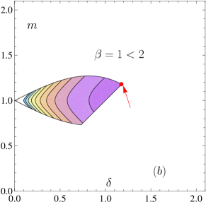
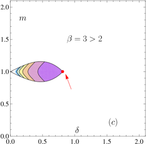
Figure 2: Contour plots of the free energy in regions of the parameter space such that ϕ(x)0italic-ϕ𝑥0\phi(x)\geq 0, for (a) β=0𝛽0\beta=0, (b) β=1𝛽1\beta=1 and (c) β=3𝛽3\beta=3. Darker regions have lower free energy. The arrows point at the minima.

By using the constraint (10), that is

11λϕ(x)𝑑x=1,superscriptsubscript11𝜆italic-ϕ𝑥differential-d𝑥1\int_{-1}^{1}\lambda\,\phi(x)\,dx=1, (20)

we can fix the Lagrange multiplier to obtain

ϕ(x)=1π1x2[1+βδ22+2(1m)δxβδ2x2].italic-ϕ𝑥1𝜋1superscript𝑥2delimited-[]1𝛽superscript𝛿2221𝑚𝛿𝑥𝛽superscript𝛿2superscript𝑥2\phi(x)=\frac{1}{\pi\sqrt{1-x^{2}}}\left[1+\frac{\beta\delta^{2}}{2}+\frac{2(1-m)}{\delta}x-\beta\delta^{2}x^{2}\right]. (21)

The physical solutions must have a density ϕ(x)italic-ϕ𝑥\phi(x) that is nonnegative for all x(1,1)𝑥11x\in(-1,1). Let us look at the points where the density vanishes, ϕ(x)=0italic-ϕ𝑥0\phi(x)=0. From (21) one gets

x±=1βδ2(1mδ±Δ),subscript𝑥plus-or-minus1𝛽superscript𝛿2plus-or-minus1𝑚𝛿Δx_{\pm}=\frac{1}{\beta\delta^{2}}\left(\frac{1-m}{\delta}\pm\sqrt{\Delta}\right), (22)

where

Δ=(1mδ)2+βδ2(1+βδ22).Δsuperscript1𝑚𝛿2𝛽superscript𝛿21𝛽superscript𝛿22\Delta=\left(\frac{1-m}{\delta}\right)^{2}+\beta\delta^{2}\left(1+\frac{\beta\delta^{2}}{2}\right). (23)

For β0𝛽0\beta\geq 0 one gets that Δ0Δ0\Delta\geq 0 for every m𝑚m and δ𝛿\delta, and ϕ(x)0italic-ϕ𝑥0\phi(x)\geq 0 for x[x,x+]𝑥subscript𝑥subscript𝑥x\in[x_{-},x_{+}]. The level curves x±=±1subscript𝑥plus-or-minusplus-or-minus1x_{\pm}=\pm 1 are given by m=Γ1±(δ,β)𝑚superscriptsubscriptΓ1plus-or-minus𝛿𝛽m=\Gamma_{1}^{\pm}(\delta,\beta), where

Γ1±(δ,β)=1±δ2(1βδ22).superscriptsubscriptΓ1plus-or-minus𝛿𝛽plus-or-minus1𝛿21𝛽superscript𝛿22\displaystyle\Gamma_{1}^{\pm}(\delta,\beta)=1\pm\frac{\delta}{2}\left(1-\frac{\beta\delta^{2}}{2}\right). (24)

They are symmetric with respect to the line m=1𝑚1m=1 and intersect at δ=0𝛿0\delta=0 and at δ=2/β𝛿2𝛽\delta=\sqrt{2/\beta}. Therefore, the condition (1,1)[x1,x2]11subscript𝑥1subscript𝑥2(-1,1)\subset[x_{1},x_{2}] implies that the points (δ,m)𝛿𝑚(\delta,m) should be restricted to a (possibly cut) “eye-shaped” domain given by

max{δ,Γ1(δ,β)}mΓ1+(δ,β),𝛿superscriptsubscriptΓ1𝛿𝛽𝑚superscriptsubscriptΓ1𝛿𝛽\max\left\{\delta,\Gamma_{1}^{-}(\delta,\beta)\right\}\leq m\leq\Gamma_{1}^{+}(\delta,\beta), (25)

(recall the constraint mδ𝑚𝛿m\geq\delta in (15) that expresses the positivity of eigenvalues). The right corner of the eye is at

(δ,m)=(2β,1),𝛿𝑚2𝛽1(\delta,m)=\left(\sqrt{\frac{2}{\beta}},1\right), (26)

and belongs to the boundary as long as β2𝛽2\beta\geq 2. For β<2𝛽2\beta<2 the eye is cut by the line m=δ𝑚𝛿m=\delta. See Fig. 1.

Let us remark that all points inside the region correspond to solutions of the saddle point equations. In other words we have a two parameter continuous family of solutions. We will look at the eigenvalue density that minimizes the free energy density of the system. From Eqs. (8) and (10) with α=3𝛼3\alpha=3 by applying the scaling (12) we get

fNsubscript𝑓𝑁\displaystyle f_{N} =\displaystyle= FN2=1Niλ(ti)22N2βi<jln|λ(ti)λ(tj)|𝐹superscript𝑁21𝑁subscript𝑖𝜆superscriptsubscript𝑡𝑖22superscript𝑁2𝛽subscript𝑖𝑗𝜆subscript𝑡𝑖𝜆subscript𝑡𝑗\displaystyle\frac{F}{N^{2}}=\frac{1}{N}\sum_{i}\lambda(t_{i})^{2}-\frac{2}{N^{2}\beta}\sum_{i<j}\ln|\lambda(t_{i})-\lambda(t_{j})| (27)
+2N2βi<jlnN2superscript𝑁2𝛽subscript𝑖𝑗𝑁\displaystyle+\frac{2}{N^{2}\beta}\sum_{i<j}\ln N
=\displaystyle= u1βs+lnN+𝒪(lnNN)𝑢1𝛽𝑠𝑁𝒪𝑁𝑁\displaystyle u-\frac{1}{\beta}s+\ln N+{\cal O}\left(\frac{\ln N}{N}\right)
=\displaystyle= f+lnN+𝒪(lnNN).𝑓𝑁𝒪𝑁𝑁\displaystyle f+\ln N+{\cal O}\left(\frac{\ln N}{N}\right).

Here,

f=limN(fN1βlnN)𝑓subscript𝑁subscript𝑓𝑁1𝛽𝑁f=\lim_{N\to\infty}\left(f_{N}-\frac{1}{\beta}\ln N\right) (28)

is the free energy density in the thermodynamic limit, which reads

βf=βus,𝛽𝑓𝛽𝑢𝑠\beta f=\beta u-s, (29)

in terms of the internal energy density u𝑢u and the entropy density s𝑠s,

u𝑢\displaystyle u =\displaystyle= 11λ2ϕ(x)𝑑x,superscriptsubscript11superscript𝜆2italic-ϕ𝑥differential-d𝑥\displaystyle\int_{-1}^{1}\lambda^{2}\phi(x)dx,
s𝑠\displaystyle s =\displaystyle= 11𝑑x11𝑑yϕ(x)ϕ(y)ln(δ|xy|).superscriptsubscript11differential-d𝑥superscriptsubscript11differential-d𝑦italic-ϕ𝑥italic-ϕ𝑦𝛿𝑥𝑦\displaystyle\int_{-1}^{1}dx\int_{-1}^{1}dy\ \phi(x)\phi(y)\ln(\delta|x-y|). (30)
Refer to caption
Refer to caption
Refer to caption
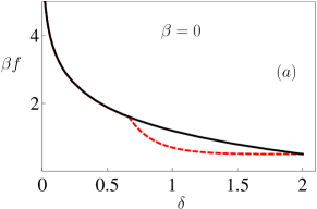
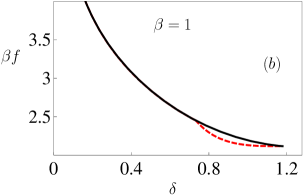
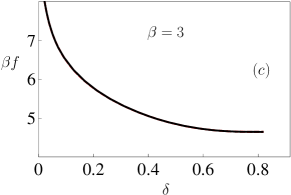
Figure 3: Free energy on the boundary of the region of the domain where ϕ(x)0italic-ϕ𝑥0\phi(x)\geq 0, for different temperatures (indicated). Dashed line: free energy f𝑓f on the lower boundary of the eye-shaped domain; full line: free energy on the upper boundary. The sought minima of the free energy can be inferred from the graph and coincide with the dots in Figs. 1 and 2.

In order to compute the entropy density one integrates the Tricomi equation (17) and obtains

11ϕ(x)𝑑x11ϕ(y)𝑑yln|yx|superscriptsubscript11italic-ϕ𝑥differential-d𝑥superscriptsubscript11italic-ϕ𝑦differential-d𝑦𝑦𝑥\displaystyle\int_{-1}^{1}\phi(x)dx\int_{-1}^{1}\phi(y)dy\ln|y-x|
=11𝑑xϕ(x)ln(x+1)absentsuperscriptsubscript11differential-d𝑥italic-ϕ𝑥𝑥1\displaystyle=\int_{-1}^{1}dx\phi(x)\ln(x+1)
π11𝑑xϕ(x)1xg(y)𝑑y.𝜋superscriptsubscript11differential-d𝑥italic-ϕ𝑥superscriptsubscript1𝑥𝑔𝑦differential-d𝑦\displaystyle\quad-\pi\int_{-1}^{1}dx\phi(x)\int_{-1}^{x}g(y)dy. (31)

We get

u(δ,m,β)𝑢𝛿𝑚𝛽\displaystyle u(\delta,m,\beta) =\displaystyle= 1(1m)2+δ22βδ48,1superscript1𝑚2superscript𝛿22𝛽superscript𝛿48\displaystyle 1-(1-m)^{2}+\frac{\delta^{2}}{2}-\frac{\beta\delta^{4}}{8}, (32)
s(δ,m,β)𝑠𝛿𝑚𝛽\displaystyle s(\delta,m,\beta) =\displaystyle= 2(1m)2δ2β2δ416+lnδ2,2superscript1𝑚2superscript𝛿2superscript𝛽2superscript𝛿416𝛿2\displaystyle-\frac{2(1-m)^{2}}{\delta^{2}}-\frac{\beta^{2}\delta^{4}}{16}+\ln{\frac{\delta}{2}}, (33)

and thus

βf(δ,m,β)𝛽𝑓𝛿𝑚𝛽\displaystyle\beta f(\delta,m,\beta) =\displaystyle= ββ(1m)2+2(1m)2δ2+βδ22𝛽𝛽superscript1𝑚22superscript1𝑚2superscript𝛿2𝛽superscript𝛿22\displaystyle\beta-\beta(1-m)^{2}+\frac{2(1-m)^{2}}{\delta^{2}}+\frac{\beta\delta^{2}}{2} (34)
β2δ416lnδ2.superscript𝛽2superscript𝛿416𝛿2\displaystyle-\frac{\beta^{2}\delta^{4}}{16}-\ln{\frac{\delta}{2}}.

The contour plots of the free energy are shown in Fig. 2. Note that f𝑓f, as well as u𝑢u and s𝑠s, is symmetric with respect to the line m=1𝑚1m=1. This 2subscript2\mathbb{Z}_{2} symmetry will play a major role in the following. The only stationary point (a saddle point) of the free energy density f𝑓f is at the right corner of the eye (26), see Figs. 1 and 2. Thus, the absolute minimum is on the boundary.

For ββ+𝛽subscript𝛽\beta\geq\beta_{+}, where

β+=2,subscript𝛽2\beta_{+}=2, (35)

the point (26) is also the absolute minimum, whereas for 0<β<β+0𝛽subscript𝛽0<\beta<\beta_{+} the absolute minimum is at the right upper corner of the allowed region, δ=Γ1+(δ,β)𝛿superscriptsubscriptΓ1𝛿𝛽\delta=\Gamma_{1}^{+}(\delta,\beta), namely at

m=δ,withβδ34+δ21=0.formulae-sequence𝑚𝛿with𝛽superscript𝛿34𝛿210m=\delta,\quad\mbox{with}\quad\beta\frac{\delta^{3}}{4}+\frac{\delta}{2}-1=0. (36)

See the dots in Figs. 1 and 2. The behavior of the free energy at the boundaries of the allowed domain is shown in Fig. 3 for different temperatures.

Refer to caption
Refer to caption
Figure 4: (Up) Density of the eigenvalues for ββ+=2𝛽subscript𝛽2\beta\geq\beta_{+}=2. (Down) Density of the eigenvalues for β=2,4𝛽24\beta=2,4 and 101010. In the temperatures range β[2,]𝛽2\beta\in[2,\infty] the solution is given by the semicircle law.

We will study the behavior of our system starting from high values of β𝛽\beta, that is low values of internal energy u𝑢u (purity). The analysis of lower values of β𝛽\beta, down to β=0𝛽0\beta=0 and even below, will be done in the next section. For β>β+𝛽subscript𝛽\beta>\beta_{+}, by setting from (26) m=1𝑚1m=1 and

β=2δ2𝛽2superscript𝛿2\beta=\frac{2}{\delta^{2}} (37)

and recalling (21), one gets the semicircle law (see Fig. 4)

ϕ(x)=2π1x2,italic-ϕ𝑥2𝜋1superscript𝑥2\phi(x)=\frac{2}{\pi}\sqrt{1-x^{2}}, (38)

whence, by (16),

ρ(λ)=βπλabλ,𝜌𝜆𝛽𝜋𝜆𝑎𝑏𝜆\rho(\lambda)=\frac{\beta}{\pi}\sqrt{\lambda-a}\sqrt{b-\lambda}, (39)

where

a=1δ=1β+β,b=1+δ=1+β+β.formulae-sequence𝑎1𝛿1subscript𝛽𝛽𝑏1𝛿1subscript𝛽𝛽a=1-\delta=1-\sqrt{\frac{\beta_{+}}{\beta}},\qquad b=1+\delta=1+\sqrt{\frac{\beta_{+}}{\beta}}. (40)

This distribution is displayed in Fig. 4. Observe that as β𝛽\beta becomes larger the distribution becomes increasingly peaked around 1. This simply means that all eigenvalues tend to 1/N1𝑁1/N in the natural scaling (12): for temperatures T=1/β𝑇1𝛽T=1/\beta close to zero the quantum state becomes maximally entangled.

By plugging (26) into (32) and (33) we get for β>β+𝛽subscript𝛽\beta>\beta_{+}

u𝑢\displaystyle u =\displaystyle= 1+δ24=1+12β,1superscript𝛿24112𝛽\displaystyle 1+\frac{\delta^{2}}{4}=1+\frac{1}{2\beta}, (41)
s𝑠\displaystyle s =\displaystyle= 14+lnδ2=1412ln(2β),14𝛿214122𝛽\displaystyle-\frac{1}{4}+\ln\frac{\delta}{2}=-\frac{1}{4}-\frac{1}{2}\ln(2\beta), (42)

and thus

βf=2δ2+34lnδ2=β+34+12ln(2β).𝛽𝑓2superscript𝛿234𝛿2𝛽34122𝛽\beta f=\frac{2}{\delta^{2}}+\frac{3}{4}-\ln\frac{\delta}{2}=\beta+\frac{3}{4}+\frac{1}{2}\ln(2\beta). (43)
Refer to caption
Refer to caption
Figure 5: (Up) Density of the eigenvalues for β=1𝛽1\beta=1. (Down) Density of eigenvalues for β=0𝛽0\beta=0, β=2/3𝛽23\beta=2/3, and β=βg=2/27𝛽subscript𝛽𝑔227\beta=\beta_{g}=-2/27 (dashed). In the range of temperatures β(βg,β+)𝛽subscript𝛽𝑔subscript𝛽\beta\in(\beta_{g},\beta_{+}), with β+=2subscript𝛽2\beta_{+}=2, the solution is given by the Wishart distribution.
Refer to caption
Figure 6: Plot of Eq. (46) for positive (solid line) and negative (dashed line) temperatures. The minimum βg=2/27subscript𝛽𝑔227\beta_{g}=-2/27 is attained at δ=3𝛿3\delta=3.

At higher temperatures 0ββ+0𝛽subscript𝛽0\leq\beta\leq\beta_{+} the solution acquires a different physiognomy. By plugging (36) into (21)

ϕ(x)=2πδ1x1+x(1+(2δ)x),italic-ϕ𝑥2𝜋𝛿1𝑥1𝑥12𝛿𝑥\phi(x)=\frac{2}{\pi\delta}\sqrt{\frac{1-x}{1+x}}\big{(}1+(2-\delta)x\big{)}, (44)

see Fig. 5, yielding, by (16),

ρ(λ)=4πb2bλλ(b2+2(4b)bλ),𝜌𝜆4𝜋superscript𝑏2𝑏𝜆𝜆𝑏224𝑏𝑏𝜆\rho(\lambda)=\frac{4}{\pi b^{2}}\sqrt{\frac{b-\lambda}{\lambda}}\left(b-2+\frac{2(4-b)}{b}\lambda\right), (45)

with b=2δ𝑏2𝛿b=2\delta. This is a Wishart distribution. See Fig. 5. The change from semicircle to Wishart is accompanied by a phase transition (the first of a series!) as we shall presently see.

The half width δ=b/2𝛿𝑏2\delta=b/2 is related to β𝛽\beta by (36)

β=4δ32δ2,𝛽4superscript𝛿32superscript𝛿2\beta=\frac{4}{\delta^{3}}-\frac{2}{\delta^{2}}, (46)

which runs monotonically from β=2𝛽2\beta=2 when δ=1𝛿1\delta=1 to β=0𝛽0\beta=0 when δ=2𝛿2\delta=2. Moreover, it reaches a minimum equal to

βg=227subscript𝛽𝑔227\beta_{g}=-\frac{2}{27} (47)

at δ=3𝛿3\delta=3. Therefore, the above solution can be smoothly extended down to βgsubscript𝛽𝑔\beta_{g}, which is slightly negative, but not below. See Fig. 6. We will study the solution for negative temperatures in the next section. Note, incidentally, that the inverse function of (46) can be explicitly written

δ(β)=1β2β3(Δ~1Δ~),𝛿𝛽1𝛽2𝛽3~Δ1~Δ\displaystyle\delta(\beta)=\frac{1}{\beta}\sqrt{\frac{2\beta}{3}}\left(\tilde{\Delta}-\frac{1}{\tilde{\Delta}}\right), (48)

with Δ~=(β/βg+1β/βg)1/3~Δsuperscript𝛽subscript𝛽𝑔1𝛽subscript𝛽𝑔13\tilde{\Delta}=(\sqrt{-\beta/\beta_{g}}+\sqrt{1-\beta/\beta_{g}})^{1/3}.

For ββ+𝛽subscript𝛽\beta\leq\beta_{+} the internal energy (average purity) u𝑢u is obtained by plugging (46) into (32)

u=32δδ24.𝑢32𝛿superscript𝛿24u=\frac{3}{2}\delta-\frac{\delta^{2}}{4}. (49)

Therefore, at β=0𝛽0\beta=0 (δ=2𝛿2\delta=2) one gets u=2𝑢2u=2, at β+=2subscript𝛽2\beta_{+}=2 (δ=1𝛿1\delta=1) one gets u=5/4𝑢54u=5/4, and at βg=2/27subscript𝛽𝑔227\beta_{g}=-2/27 (δ=3𝛿3\delta=3) one gets u=9/4𝑢94u=9/4 (see the next section for the significance of these values). From (46) and (33) one can also compute the entropy and the free energy for ββ+𝛽subscript𝛽\beta\leq\beta_{+}

s𝑠\displaystyle s =\displaystyle= 94+5δ3δ2+lnδ2,945𝛿3superscript𝛿2𝛿2\displaystyle-\frac{9}{4}+\frac{5}{\delta}-\frac{3}{\delta^{2}}+\ln\frac{\delta}{2}, (50)
βf𝛽𝑓\displaystyle\beta f =\displaystyle= 9δ29δ+114lnδ2,9superscript𝛿29𝛿114𝛿2\displaystyle\frac{9}{\delta^{2}}-\frac{9}{\delta}+\frac{11}{4}-\ln\frac{\delta}{2}, (51)

in terms of the function δ(β)(1,3]𝛿𝛽13\delta(\beta)\in(1,3] introduced in Eq. (48).

Notice that βf𝛽𝑓\beta f is the generating function for the connected correlations of πABsubscript𝜋𝐴𝐵\pi_{AB}. The radius of convergence in the expansion around β=0𝛽0\beta=0, namely 2/272272/27, defines the behavior of the late terms in the cumulants series. Another interesting observation is that the function r(x)=u(β=x/2)𝑟𝑥𝑢𝛽𝑥2r(x)=u(\beta=-x/2) is the generating function of the number of rooted non-separable planar maps with n𝑛n edges on the sphere (Sloane’s A000139 also in Tutte ; BM ), namely

r(x)𝑟𝑥\displaystyle r(x) =\displaystyle= 2+x+2x2+6x3+22x4+91x5+408x62𝑥2superscript𝑥26superscript𝑥322superscript𝑥491superscript𝑥5408superscript𝑥6\displaystyle 2+x+2x^{2}+6x^{3}+22x^{4}+91x^{5}+408x^{6} (52)
+1,938x7+9,614x8+49,335x9+.1938superscript𝑥79614superscript𝑥849335superscript𝑥9\displaystyle+1,938x^{7}+9,614x^{8}+49,335x^{9}+...\ .

The counting of rooted planar maps on higher genus surfaces is an unsolved problem in combinatorics and we conjecture it to be related to 1/N1𝑁1/N corrections of our formulas.

We are now ready to unveil the presence of the first critical point at β+=2subscript𝛽2\beta_{+}=2. Let consider the density of eigenvalues (38) and (44) (or their counterpart (39) and (45)). The phase transition at β+subscript𝛽\beta_{+} is due to the restoration of a 2subscript2{\mathbb{Z}}_{2} symmetry P𝑃P (“parity”) present in Eqs.  (32), (33) and (34), namely the reflection of the distribution ρ(λ)𝜌𝜆\rho(\lambda) around the center of its support (m=δ=b/2𝑚𝛿𝑏2m=\delta=b/2 for ββ+𝛽subscript𝛽\beta\leq\beta_{+} and m=1𝑚1m=1 for β>β+𝛽subscript𝛽\beta>\beta_{+}). For ββ+𝛽subscript𝛽\beta\leq\beta_{+} there are two solutions linked by this symmetry, and we picked the one with the lowest f𝑓f; at β+subscript𝛽\beta_{+} this two solutions coincide with the semicircle (39), which is invariant under P𝑃P and becomes the valid and stable solution for higher β𝛽\beta. In order to explicitly show the presence of a second order phase transition in the system for β=β+𝛽subscript𝛽\beta=\beta_{+} we look at the expression of the entropy density s=β(uf)𝑠𝛽𝑢𝑓s=\beta(u-f), which counts the number of states with a given value of the purity. The expression for β<β+𝛽subscript𝛽\beta<\beta_{+} is given in Eq. (50), while for ββ+𝛽subscript𝛽\beta\geq\beta_{+} it is given in Eq. (42).

At β=β+𝛽subscript𝛽\beta=\beta_{+} we get δ=1𝛿1\delta=1 and s=1/4ln2𝑠142s=-1/4-\ln 2. On the other hand the first derivative of s𝑠s with respect to δ𝛿\delta is discontinuous at δ=1𝛿1\delta=1. However, also β𝛽\beta as a function of δ𝛿\delta, as given by (46) and (37), has a discontinuous first derivative at δ=1𝛿1\delta=1. By recalling that

dsdβ𝑑𝑠𝑑𝛽\displaystyle\frac{ds}{d\beta} =\displaystyle= dsdδ/dβdδ,𝑑𝑠𝑑𝛿𝑑𝛽𝑑𝛿\displaystyle\frac{ds}{d\delta}\Big{/}\frac{d\beta}{d\delta},
d2sdβ2superscript𝑑2𝑠𝑑superscript𝛽2\displaystyle\frac{d^{2}s}{d\beta^{2}} =\displaystyle= d2sdδ2/(dβdδ)2dsdδd2βdδ2/(dβdδ)3,superscript𝑑2𝑠𝑑superscript𝛿2superscript𝑑𝛽𝑑𝛿2𝑑𝑠𝑑𝛿superscript𝑑2𝛽𝑑superscript𝛿2superscript𝑑𝛽𝑑𝛿3\displaystyle\frac{d^{2}s}{d\delta^{2}}\Big{/}\left(\frac{d\beta}{d\delta}\right)^{2}-\frac{ds}{d\delta}\,\frac{d^{2}\beta}{d\delta^{2}}\Big{/}\left(\frac{d\beta}{d\delta}\right)^{3}, (53)

one easily obtains that the discontinuities compensate and in the critical region, ββ+𝛽subscript𝛽\beta\to\beta_{+}, we have

s14ln2ββ+4+θ(ββ+)(ββ+)216,similar-to𝑠142𝛽subscript𝛽4𝜃𝛽subscript𝛽superscript𝛽subscript𝛽216\displaystyle s\sim-\frac{1}{4}-\ln 2-\frac{\beta-\beta_{+}}{4}+\theta(\beta-\beta_{+})\frac{(\beta-\beta_{+})^{2}}{16},\; (54)

where θ𝜃\theta is the step function. The entropy s𝑠s is continuous at the phase transition, together with its first derivative, although the second derivative is discontinuous, as shown in Fig. 7.

Refer to caption
Refer to caption
Figure 7: Entropy and its second derivative with respect to β𝛽\beta. The entropy is continuous in β+subscript𝛽\beta_{+} while its second derivative presents a finite discontinuity.

Notice that the entropy is unbounded from below when β+𝛽\beta\to+\infty. The interpretation of this result is quite straightforward: the minimum value of πABsubscript𝜋𝐴𝐵\pi_{AB} is reached on a submanifold (isomorphic to SU(N)/ZN𝑆𝑈𝑁subscript𝑍𝑁SU(N)/Z_{N} Kus01 ) of dimension N21superscript𝑁21N^{2}-1, as opposed to the typical vectors which form a manifold of dimension 2N2N12superscript𝑁2𝑁12N^{2}-N-1 in the Hilbert space \mathcal{H}. Since this manifold has zero volume in the original Hilbert space, the entropy, being the logarithm of this volume, diverges.

Now we want to express the entropy density s𝑠s as a function of the internal energy density u𝑢u. From (49) and (41) we get

u={1+δ24,0<δ1,32δδ24,1<δ2,𝑢cases1superscript𝛿240𝛿1otherwiseotherwise32𝛿superscript𝛿241𝛿2u=\begin{cases}1+\frac{\delta^{2}}{4},&0<\delta\leq 1,\\ \\ \frac{3}{2}\delta-\frac{\delta^{2}}{4},&1<\delta\leq 2,\end{cases} (55)

that can be easily inverted

δ={2u1,1<u54,394u,54<u2.𝛿cases2𝑢11𝑢54otherwiseotherwise394𝑢54𝑢2\delta=\begin{cases}2\sqrt{u-1},&1<u\leq\frac{5}{4},\\ \\ 3-\sqrt{9-4u},&\frac{5}{4}<u\leq 2.\end{cases} (56)

From (50) and (42) one gets the entropy density as a function of δ𝛿\delta

s={14+lnδ2,0<δ1,94+5δ3δ2+lnδ2,1<δ2.𝑠cases14𝛿20𝛿1otherwiseotherwise945𝛿3superscript𝛿2𝛿21𝛿2s=\begin{cases}-\frac{1}{4}+\ln\frac{\delta}{2},&0<\delta\leq 1,\\ \\ -\frac{9}{4}+\frac{5}{\delta}-\frac{3}{\delta^{2}}+\ln\frac{\delta}{2},&1<\delta\leq 2.\end{cases} (57)

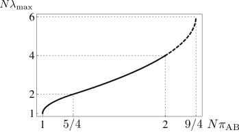
Finally, by plugging (56) into (57), we obtain the entropy of the submanifold of fixed purity, s=(lnV)/N2𝑠𝑉superscript𝑁2s=(\ln V)/N^{2} as a function of its internal energy u=NπAB𝑢𝑁subscript𝜋𝐴𝐵u=N\pi_{AB}:

s(u)={12ln(u1)14,1u54,ln(3294u)94+52(3294u)34(3294u)2,54u2.𝑠𝑢cases12𝑢1141𝑢54otherwiseotherwise3294𝑢94523294𝑢34superscript3294𝑢254𝑢2\displaystyle s(u)=\begin{cases}\frac{1}{2}\ln(u-1)-\frac{1}{4},&1\leq u\leq\frac{5}{4},\\ \\ \ln\left(\frac{3}{2}-\sqrt{\frac{9}{4}-u}\right)-\frac{9}{4}+\frac{5}{2\left(\frac{3}{2}-\sqrt{\frac{9}{4}-u}\right)}-\frac{3}{4\left(\frac{3}{2}-\sqrt{\frac{9}{4}-u}\right)^{2}},&\frac{5}{4}\leq u\leq 2.\end{cases} (58)

This function is plotted in Fig. 8.

Refer to caption
Figure 8: Entropy density s𝑠s versus internal energy density u=NπAB𝑢𝑁delimited-⟨⟩subscript𝜋𝐴𝐵u=N\langle\pi_{AB}\rangle. See Eq. (58).

Let us discuss the significance of these results. The present section was devoted to the study of positive temperatures T=1/β>0𝑇1𝛽0T=1/\beta>0. In this range of temperatures, the eigenvalues of the reduced density matrix of our N2superscript𝑁2N^{2}-dimensional system are always of 𝒪(1/N)𝒪1𝑁{\cal O}\left(1/N\right). As a consequence, the value of energy (purity) in Eq. (2)

πAB=j=1Nλj21Nλ2ρ(λ)𝑑λ=𝒪(1N)subscript𝜋𝐴𝐵superscriptsubscript𝑗1𝑁superscriptsubscript𝜆𝑗2similar-to-or-equals1𝑁superscript𝜆2𝜌𝜆differential-d𝜆𝒪1𝑁\pi_{AB}=\sum_{j=1}^{N}\lambda_{j}^{2}\simeq\frac{1}{N}\int\lambda^{2}\rho(\lambda)d\lambda={\cal O}\left(\frac{1}{N}\right) (59)

is always small: there is therefore a lot of entanglement in our system. There are however, important differences as purity changes (it is important to keep in mind that in the statistical mechanical approach pursued here, the Lagrange multiplier β𝛽\beta fixes the value of energy/purity). When 1/N<πAB<5/4N1𝑁subscript𝜋𝐴𝐵54𝑁1/N<\pi_{AB}<5/4N the eigenvalues are distributed according to the semicircle law (Fig. 4), while for 5/4N<πAB<2/N54𝑁subscript𝜋𝐴𝐵2𝑁5/4N<\pi_{AB}<2/N they follow the Wishart distribution (Fig. 5), the two regimes being separated by a second-order phase transition. The value πAB=2/Nsubscript𝜋𝐴𝐵2𝑁\pi_{AB}=2/N corresponds to infinite temperatures β=0𝛽0\beta=0 and therefore to typical vectors in the Hilbert space (according to the Haar measure). One is therefore tempted to extend these results to negative temperatures paper1 and one can indeed do so up to πAB=9/4Nsubscript𝜋𝐴𝐵94𝑁\pi_{AB}=9/4N, corresponding to the slightly negative temperature βg=2/27subscript𝛽𝑔227\beta_{g}=-2/27. However, as we have seen, a mathematical difficulty emerges, as this value represents the radius of convergence of an expansion around β=0𝛽0\beta=0 and no smooth continuation of this solution seems possible beyond βgsubscript𝛽𝑔\beta_{g}. In the next section we will see that two branches exist for negative β𝛽\beta: one containing the point β=βg𝛽subscript𝛽𝑔\beta=\beta_{g} and in which purity is always of 𝒪(1/N)𝒪1𝑁{\cal O}\left(1/N\right) and one in which purity is of 𝒪(1)𝒪1{\cal O}\left(1\right). The latter becomes stable for sufficiently large β𝛽-\beta’s through a first order phase transition.

Before continuing, we remind that larger values of purity, towards the regime πAB=𝒪(1)subscript𝜋𝐴𝐵𝒪1\pi_{AB}={\cal O}\left(1\right) yield separable (factorized) states. We are therefore going to look at the behavior of our quantum system towards separability (regime of small entanglement).

IV Negative temperatures

IV.1 Metastable branch (quantum gravity)

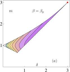
By analytic continuation, the solution at positive β𝛽\beta of the previous subsection can be turned into a solution for negative β𝛽\beta, satisfying the constraints of positivity and normalization. In this section we will study this analytic continuation and its phase transitions, but we anticipate that this is metastable for sufficiently large β𝛽-\beta’s (namely for β<2.455/N𝛽2.455𝑁\beta<-2.455/N) and that it will play a secondary role in the thermodynamics of our model. However, our interest in it is spurred by one of its critical points, at β=2/27βg𝛽227subscript𝛽𝑔\beta=-2/27\equiv\beta_{g} which corresponds to the so-called 2-D quantum gravity free energy (see Di Francesco:1993nw ), provided an appropriate double-scaling limit (jointly ββg𝛽subscript𝛽𝑔\beta\to\beta_{g} and N𝑁N\to\infty) is performed.

In more details, the eigenvalue density (45) at β=βg=2/27𝛽subscript𝛽𝑔227\beta=\beta_{g}=-2/27, i.e. δ=3𝛿3\delta=3 [see between Eqs. (46) and (48), and Fig. 6] reads

ρ(λ)=227π(6λ)3λ,𝜌𝜆227𝜋superscript6𝜆3𝜆\rho(\lambda)=\frac{2}{27\pi}\sqrt{\frac{(6-\lambda)^{3}}{\lambda}}, (60)

and from (49) u=9/4𝑢94u=9/4 (see Fig. 7 and 9). The derivative at the right edge of eigenvalue density in Fig. 5 vanishes.

By expanding (46) for δ3𝛿3\delta\to 3

β𝛽\displaystyle\beta =\displaystyle= 227+281(δ3)216729(δ3)3+10729(δ3)4227281superscript𝛿3216729superscript𝛿3310729superscript𝛿34\displaystyle-\frac{2}{27}+\frac{2}{81}(\delta-3)^{2}-\frac{16}{729}(\delta-3)^{3}+\frac{10}{729}(\delta-3)^{4} (61)
162187(δ3)5+𝒪((δ3)6),162187superscript𝛿35𝒪superscript𝛿36\displaystyle-\frac{16}{2187}(\delta-3)^{5}+{\cal O}\left((\delta-3)^{6}\right),

that is, by setting x=2(ββg)/90𝑥2𝛽subscript𝛽𝑔90x=\sqrt{2(\beta-\beta_{g})/9}\,\to 0,

δ=3(1+x+43x2+3518x3+8027x4+1001216x5+𝒪(x6)),𝛿31𝑥43superscript𝑥23518superscript𝑥38027superscript𝑥41001216superscript𝑥5𝒪superscript𝑥6\delta=3\left(1+x+\frac{4}{3}x^{2}+\frac{35}{18}x^{3}+\frac{80}{27}x^{4}+\frac{1001}{216}x^{5}+{\cal O}\left(x^{6}\right)\right), (62)

and therefore for ββg𝛽subscript𝛽𝑔\beta\to\beta_{g}

βf𝛽𝑓\displaystyle\beta f =\displaystyle= 34log32+94(ββg)8116(ββg)2343294𝛽subscript𝛽𝑔8116superscript𝛽subscript𝛽𝑔2\displaystyle\frac{3}{4}-\log\frac{3}{2}+\frac{9}{4}(\beta-\beta_{g})-\frac{81}{16}(\beta-\beta_{g})^{2} (63)
8125(ββg)5/2+𝒪((ββg)3).8125superscript𝛽subscript𝛽𝑔52𝒪superscript𝛽subscript𝛽𝑔3\displaystyle-\frac{81\sqrt{2}}{5}(\beta-\beta_{g})^{5/2}+{\cal O}\left((\beta-\beta_{g})^{3}\right).

In fact, if one relaxes the unit trace condition, our partition function 𝒵𝒵{\cal Z} has been studied in the context of random matrix theories Morris91 before. The objects generated in this way correspond to chequered polygonations of surfaces. Our calculations show that the constraint TrρA=1Trsubscript𝜌𝐴1{\rm Tr}\ \rho_{A}=1 is irrelevant for the critical exponents in this region.

However, this is not a real critical point of our Coulomb gas. As this is an analytic continuation of the solution obtained for β>0𝛽0\beta>0, we are not assured that this is indeed a stable branch. In the next section we will show that a first order phase transition occurs at a lower value of β𝛽\beta, namely at β2.455/Nsimilar-to-or-equals𝛽2.455𝑁\beta\simeq-2.455/N in this scaling (and therefore the exponent α𝛼\alpha needs to be lowered from 3 to 2 for negative β𝛽\beta). The new stable phase will take over for all negative β𝛽\beta, where β=𝛽\beta=-\infty corresponds to separable states. However the analytic continuation described here, although metastable, exists for all negative β𝛽\beta and we can study in more detail the behavior of the eigenvalue density (21) and of its free energy (34). The solution is straightforward but lengthy and is given in the following. It is of interest in itself because, as we shall see, it entails a restoration of the 2subscript2\mathbb{Z}_{2} symmetry that was broken at the phase transition at β=2𝛽2\beta=2 described in the previous section.

Refer to caption
Figure 9: u=NπAB𝑢𝑁delimited-⟨⟩subscript𝜋𝐴𝐵u=N\langle\pi_{AB}\rangle as a function of (inverse) temperature. Notice that u=2𝑢2u=2 at β=0𝛽0\beta=0 (typical states). In the β𝛽\beta\to\infty limit we find the minimum u=1𝑢1u=1. The critical points described in the text are at βg=2/27,u=9/4formulae-sequencesubscript𝛽𝑔227𝑢94\beta_{g}=-2/27,u=9/4 (left point) and β+=2,u=5/4formulae-sequencesubscript𝛽2𝑢54\beta_{+}=2,u=5/4 (right point). However this phase is unstable (dashed line) towards another phase as soon as β<0𝛽0\beta<0 (in this scaling of β𝛽\beta).
Refer to caption
Refer to caption
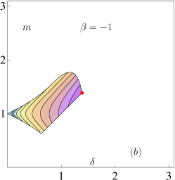
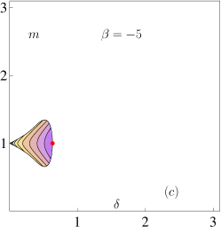
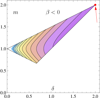
Figure 10: Metastable branch. Domain of existence for the solution (m,δ)𝑚𝛿(m,\delta) for negative temperatures.

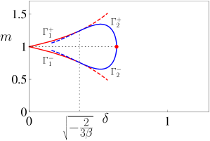
Recall that the density ϕ(x)italic-ϕ𝑥\phi(x) must be nonnegative for all x(1,1)𝑥11x\in(-1,1). This condition for β<0𝛽0\beta<0 gives x(x+,x)𝑥subscript𝑥subscript𝑥x\notin(x_{+},x_{-}), with x±subscript𝑥plus-or-minusx_{\pm} given by (22)-(23). The level curves x±=±1subscript𝑥plus-or-minusplus-or-minus1x_{\pm}=\pm 1 are given by m=Γ1±(δ,β)𝑚superscriptsubscriptΓ1plus-or-minus𝛿𝛽m=\Gamma_{1}^{\pm}(\delta,\beta), with Γ1±superscriptsubscriptΓ1plus-or-minus\Gamma_{1}^{\pm} in (24), while the level curves Δ=0Δ0\Delta=0 are given by m=Γ2±(δ,β)𝑚superscriptsubscriptΓ2plus-or-minus𝛿𝛽m=\Gamma_{2}^{\pm}(\delta,\beta) with

Γ2±(δ,β)=1±δ2β(1+βδ22),superscriptsubscriptΓ2plus-or-minus𝛿𝛽plus-or-minus1superscript𝛿2𝛽1𝛽superscript𝛿22\Gamma_{2}^{\pm}(\delta,\beta)=1\pm\delta^{2}\sqrt{-\beta\left(1+\frac{\beta\delta^{2}}{2}\right)}, (64)

They are symmetric with respect to the line m=1𝑚1m=1 and intersect at δ=0𝛿0\delta=0 and at δ=2/β𝛿2𝛽\delta=\sqrt{-2/\beta}. Moreover, they are tangent to Γ1±superscriptsubscriptΓ1plus-or-minus\Gamma_{1}^{\pm} at the points

(δ,m)=(23β, 1±2323β),𝛿𝑚23𝛽plus-or-minus12323𝛽(\delta,m)=\left(\sqrt{-\frac{2}{3\beta}},\;1\pm\frac{2}{3}\sqrt{-\frac{2}{3\beta}}\right), (65)

as shown in Fig. 10. Therefore, the condition (1,1)[x1,x2]=11subscript𝑥1subscript𝑥2(-1,1)\cap[x_{1},x_{2}]=\emptyset implies that the points (δ,m)𝛿𝑚(\delta,m) should be restricted to a (possibly cut) eye-shaped domain given by

max{δ,h(β,δ)}mh+(β,δ),𝛿subscript𝛽𝛿𝑚subscript𝛽𝛿\max\left\{\delta,\;h_{-}(\beta,\delta)\right\}\leq m\leq h_{+}(\beta,\delta), (66)

where

h±(δ,β)={Γ1±(δ,β),0δ23β,Γ2±(δ,β),δ>23β.subscriptplus-or-minus𝛿𝛽casessuperscriptsubscriptΓ1plus-or-minus𝛿𝛽0𝛿23𝛽otherwiseotherwisesuperscriptsubscriptΓ2plus-or-minus𝛿𝛽𝛿23𝛽h_{\pm}(\delta,\beta)=\begin{cases}\Gamma_{1}^{\pm}(\delta,\beta),&0\leq\delta\leq\sqrt{-\frac{2}{3\beta}},\\ \\ \Gamma_{2}^{\pm}(\delta,\beta),&\delta>\sqrt{-\frac{2}{3\beta}}.\end{cases} (67)

The right corner of the eye is given by

(δ,m)=(2β,1)𝛿𝑚2𝛽1(\delta,m)=\left(\sqrt{-\frac{2}{\beta}},1\right) (68)

and belongs to the boundary as long as β2𝛽2\beta\leq-2. For β4𝛽4\beta\geq-4 the eye is cut by the line m=δ𝑚𝛿m=\delta. See Fig. 10.

Refer to caption
Refer to caption
Refer to caption
Figure 11: Metastable branch. Contour plots of the free energy in regions of the parameter space such that ϕ(x)0italic-ϕ𝑥0\phi(x)\geq 0, for (a) β=βg𝛽subscript𝛽𝑔\beta=\beta_{g}, (b) β=1𝛽1\beta=-1 and (c) β=5𝛽5\beta=-5. Darker regions have lower free energy.

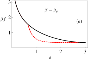
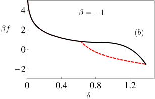
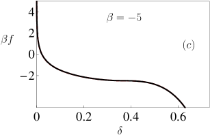
The contour plots of the free energy (34) are shown in Fig. 11. The free energy density f𝑓f has no stationary points for β<0𝛽0\beta<0. The behavior of the free energy at the boundaries of the allowed domain is shown in Fig. 12 for different temperatures. For β2𝛽2\beta\leq-2 the right corner of the eye is the absolute minimum, whereas for 2<β<02𝛽0-2<\beta<0 the absolute minimum is at the right upper corner of the allowed region, namely at

m=δ,withδ=h+(β,δ),formulae-sequence𝑚𝛿with𝛿subscript𝛽𝛿m=\delta,\quad\mbox{with}\quad\delta=h_{+}(\beta,\delta), (69)

that is

βδ34+δ21=0,for227β0,formulae-sequence𝛽superscript𝛿34𝛿210for227𝛽0\beta\frac{\delta^{3}}{4}+\frac{\delta}{2}-1=0,\quad\mbox{for}-\frac{2}{27}\leq\beta\leq 0, (70)

and

δ1=δ2β(1+βδ22),for2β227.formulae-sequence𝛿1superscript𝛿2𝛽1𝛽superscript𝛿22for2𝛽227\delta-1=\delta^{2}\sqrt{-\beta\left(1+\beta\frac{\delta^{2}}{2}\right)},\quad\mbox{for}-2\leq\beta\leq-\frac{2}{27}. (71)

Note that (70) coincides with (36) and thus is the prolongation of the curve (46) which runs monotonically from β=0𝛽0\beta=0 when δ=2𝛿2\delta=2 to its minimum βg=2/27subscript𝛽𝑔227\beta_{g}=-2/27 at δ=3𝛿3\delta=3.

Refer to caption
Refer to caption
Refer to caption
Figure 12: Metastable branch. Free energy on the boundary of the region of the domain where ϕ(x)0italic-ϕ𝑥0\phi(x)\geq 0, for different temperatures (indicated). Dashed line: free energy βf𝛽𝑓\beta f on the lower boundary of the eye-shaped domain; full line: free energy on the upper boundary. The sought minima of the free energy can be inferred from the graph and coincide with the dots in Figs. 10 and 11.

On the other hand, (71) is given by the curves

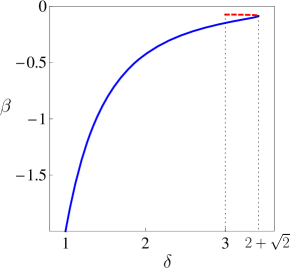
β𝛽\displaystyle\beta =\displaystyle= 1δ2±1δ3δ2+4δ2plus-or-minus1superscript𝛿21superscript𝛿3superscript𝛿24𝛿2\displaystyle-\frac{1}{\delta^{2}}\pm\frac{1}{\delta^{3}}\sqrt{-\delta^{2}+4\delta-2} (72)
=\displaystyle= 1δ2±1δ3(2+2δ)(δ2+2),plus-or-minus1superscript𝛿21superscript𝛿322𝛿𝛿22\displaystyle-\frac{1}{\delta^{2}}\pm\frac{1}{\delta^{3}}\sqrt{(2+\sqrt{2}-\delta)(\delta-2+\sqrt{2})},

which run from β=βg𝛽subscript𝛽𝑔\beta=\beta_{g} when δ=3𝛿3\delta=3 (with derivative zero) up to β=3/2+2𝛽322\beta=-3/2+\sqrt{2} when δ=2+2𝛿22\delta=2+\sqrt{2} (with derivative -\infty) and then from β=3/2+2𝛽322\beta=-3/2+\sqrt{2} when δ=2+2𝛿22\delta=2+\sqrt{2} (with derivative ++\infty) up to β=2𝛽2\beta=-2 when δ=1𝛿1\delta=1. See Fig. 13.

Refer to caption
Figure 13: Metastable branch. β𝛽\beta vs δ𝛿\delta. See Eq. (72).

Let us look at the eigenvalue density (21). When βgβ0subscript𝛽𝑔𝛽0\beta_{g}\leq\beta\leq 0 the solution is obtained by plugging (36) into (21)

ϕ(x)=2πδ1x1+x(1+(2δ)x),italic-ϕ𝑥2𝜋𝛿1𝑥1𝑥12𝛿𝑥\phi(x)=\frac{2}{\pi\delta}\sqrt{\frac{1-x}{1+x}}\big{(}1+(2-\delta)x\big{)}, (73)

with 2δ32𝛿32\leq\delta\leq 3, and is Wishart. At βgsubscript𝛽𝑔\beta_{g} one gets δ=3𝛿3\delta=3 and

ϕ(x)=23π(1x)31+x,italic-ϕ𝑥23𝜋superscript1𝑥31𝑥\phi(x)=\frac{2}{3\pi}\sqrt{\frac{(1-x)^{3}}{1+x}}, (74)

whose derivative at the right edge x=1𝑥1x=1 vanishes. On the other hand, when 3/2+2ββg322𝛽subscript𝛽𝑔-3/2+\sqrt{2}\leq\beta\leq\beta_{g} by (72) one gets

ϕ(x)=1πδ1x2[12(δ+δ2+4δ2)+2(1δ)x+(δδ2+4δ2)x2],italic-ϕ𝑥1𝜋𝛿1superscript𝑥2delimited-[]12𝛿superscript𝛿24𝛿221𝛿𝑥𝛿superscript𝛿24𝛿2superscript𝑥2\phi(x)=\frac{1}{\pi\delta\sqrt{1-x^{2}}}\left[\frac{1}{2}\left(\delta+\sqrt{-\delta^{2}+4\delta-2}\right)+2(1-\delta)x+\left(\delta-\sqrt{-\delta^{2}+4\delta-2}\right)x^{2}\right], (75)

with 3δ2+23𝛿223\leq\delta\leq 2+\sqrt{2}, while for 2β3/2+22𝛽322-2\leq\beta\leq-3/2+\sqrt{2}

ϕ(x)=1πδ1x2[12(δδ2+4δ2)+2(1δ)x+(δ+δ2+4δ2)x2],italic-ϕ𝑥1𝜋𝛿1superscript𝑥2delimited-[]12𝛿superscript𝛿24𝛿221𝛿𝑥𝛿superscript𝛿24𝛿2superscript𝑥2\phi(x)=\frac{1}{\pi\delta\sqrt{1-x^{2}}}\left[\frac{1}{2}\left(\delta-\sqrt{-\delta^{2}+4\delta-2}\right)+2(1-\delta)x+\left(\delta+\sqrt{-\delta^{2}+4\delta-2}\right)x^{2}\right], (76)

with 1δ2+21𝛿221\leq\delta\leq 2+\sqrt{2}. Note that this eigenvalue density diverge both at the left edge x=1𝑥1x=-1 and at the right edge x=+1𝑥1x=+1.

Refer to caption
Refer to caption
Refer to caption
Refer to caption
Figure 14: Metastable branch. Eigenvalue density for β=1/27𝛽127\beta=-1/27, βg=2/27subscript𝛽𝑔227\beta_{g}=-2/27, ββgless-than-or-similar-to𝛽subscript𝛽𝑔\beta\lesssim\beta_{g} and β<β=2𝛽subscript𝛽2\beta<\beta_{-}=-2. From left to right, notice how the distribution (initially Wishart, whose derivative at the rigth edge of the domain diverges) gets first a vanishing derivative at the right edge, then develops a singularity there and eventually restores the 2subscript2\mathbb{Z}_{2} symmetry that was broken at the phase transition at β=2𝛽2\beta=2 described in the previous section.

At β=2𝛽2\beta=-2 one obtains δ=1𝛿1\delta=1 and

ϕ(x)=2x2π1x2.italic-ϕ𝑥2superscript𝑥2𝜋1superscript𝑥2\phi(x)=\frac{2x^{2}}{\pi\sqrt{1-x^{2}}}. (77)

One gets the above density for all β2𝛽2\beta\leq-2, where the 2subscript2\mathbb{Z}_{2} symmetry is restored. The interesting behavior of the eigenvalue density as β𝛽\beta is varied is displayed in Fig. 14.

The values of (m,δ)𝑚𝛿(m,\delta) [that define the eigenvalue domain, see Eq. (15)] and the thermodynamic functions u𝑢u (internal energy density) and s𝑠s (entropy density) are shown in Figs. 15, 16, respectively. Their explicit expressions are given for positive temperatures in Sec. III, while for negative temperatures are given in the following.

In the gravity branch, for βgβ0subscript𝛽𝑔𝛽0\beta_{g}\leq\beta\leq 0 (2δ32𝛿32\leq\delta\leq 3) we get

m𝑚\displaystyle m =\displaystyle= δ,β=4δ32δ2,𝛿𝛽4superscript𝛿32superscript𝛿2\displaystyle\delta,\quad\beta=\frac{4}{\delta^{3}}-\frac{2}{\delta^{2}},
u𝑢\displaystyle u =\displaystyle= 32δδ24,32𝛿superscript𝛿24\displaystyle\frac{3}{2}\delta-\frac{\delta^{2}}{4},
s𝑠\displaystyle s =\displaystyle= 94+5δ3δ2+lnδ2,945𝛿3superscript𝛿2𝛿2\displaystyle-\frac{9}{4}+\frac{5}{\delta}-\frac{3}{\delta^{2}}+\ln\frac{\delta}{2},
βf𝛽𝑓\displaystyle\beta f =\displaystyle= 1149δ+9δ2lnδ2.1149𝛿9superscript𝛿2𝛿2\displaystyle\frac{11}{4}-\frac{9}{\delta}+\frac{9}{\delta^{2}}-\ln\frac{\delta}{2}. (78)

Beyond a second order phase transition at the critical temperature βgsubscript𝛽𝑔\beta_{g} we get that for 3/2+2ββg322𝛽subscript𝛽𝑔-3/2+\sqrt{2}\leq\beta\leq\beta_{g} (3δ2+23𝛿223\leq\delta\leq 2+\sqrt{2}) both u𝑢u and s𝑠s increase together with the eigenvalue density halfwidth δ𝛿\delta,

m𝑚\displaystyle m =\displaystyle= δ,β=1δ2+1δ3δ2+4δ2,𝛿𝛽1superscript𝛿21superscript𝛿3superscript𝛿24𝛿2\displaystyle\delta,\quad\beta=-\frac{1}{\delta^{2}}+\frac{1}{\delta^{3}}\sqrt{-\delta^{2}+4\delta-2},
u𝑢\displaystyle u =\displaystyle= 2δ38δ2δ8δ2+4δ2,2𝛿38superscript𝛿2𝛿8superscript𝛿24𝛿2\displaystyle 2\delta-\frac{3}{8}\delta^{2}-\frac{\delta}{8}\sqrt{-\delta^{2}+4\delta-2},
s𝑠\displaystyle s =\displaystyle= 2+154δ158δ2+18δδ2+4δ2+lnδ2,2154𝛿158superscript𝛿218𝛿superscript𝛿24𝛿2𝛿2\displaystyle-2+\frac{15}{4\delta}-\frac{15}{8\delta^{2}}+\frac{1}{8\delta}\sqrt{-\delta^{2}+4\delta-2}+\ln\frac{\delta}{2},
βf𝛽𝑓\displaystyle\beta f =\displaystyle= 52254δ+178δ2(38δ2δ2)δ2+4δ252254𝛿178superscript𝛿238𝛿2superscript𝛿2superscript𝛿24𝛿2\displaystyle\frac{5}{2}-\frac{25}{4\delta}+\frac{17}{8\delta^{2}}-\left(\frac{3}{8\delta}-\frac{2}{\delta^{2}}\right)\sqrt{-\delta^{2}+4\delta-2} (79)
lnδ2,𝛿2\displaystyle-\ln\frac{\delta}{2},

and then decrease for 2β3/2+22𝛽322-2\leq\beta\leq-3/2+\sqrt{2} (1δ2+21𝛿221\leq\delta\leq 2+\sqrt{2}),

m𝑚\displaystyle m =\displaystyle= δ,β=1δ21δ3δ2+4δ2,𝛿𝛽1superscript𝛿21superscript𝛿3superscript𝛿24𝛿2\displaystyle\delta,\quad\beta=-\frac{1}{\delta^{2}}-\frac{1}{\delta^{3}}\sqrt{-\delta^{2}+4\delta-2},
u𝑢\displaystyle u =\displaystyle= 2δ38δ2+δ8δ2+4δ2,2𝛿38superscript𝛿2𝛿8superscript𝛿24𝛿2\displaystyle 2\delta-\frac{3}{8}\delta^{2}+\frac{\delta}{8}\sqrt{-\delta^{2}+4\delta-2},
s𝑠\displaystyle s =\displaystyle= 2+154δ158δ218δδ2+4δ2+lnδ2,2154𝛿158superscript𝛿218𝛿superscript𝛿24𝛿2𝛿2\displaystyle-2+\frac{15}{4\delta}-\frac{15}{8\delta^{2}}-\frac{1}{8\delta}\sqrt{-\delta^{2}+4\delta-2}+\ln\frac{\delta}{2},
βf𝛽𝑓\displaystyle\beta f =\displaystyle= 52254δ+178δ2+(38δ2δ2)δ2+4δ252254𝛿178superscript𝛿238𝛿2superscript𝛿2superscript𝛿24𝛿2\displaystyle\frac{5}{2}-\frac{25}{4\delta}+\frac{17}{8\delta^{2}}+\left(\frac{3}{8\delta}-\frac{2}{\delta^{2}}\right)\sqrt{-\delta^{2}+4\delta-2}\qquad (80)
lnδ2.𝛿2\displaystyle-\ln\frac{\delta}{2}.

Finally, beyond another second order phase transition for β2𝛽2\beta\leq-2 (0δ10𝛿10\leq\delta\leq 1), when the 2subscript2\mathbb{Z}_{2} symmetry is restored, we get

m𝑚\displaystyle m =\displaystyle= 1,β=2δ2,1𝛽2superscript𝛿2\displaystyle 1,\quad\beta=-\frac{2}{\delta^{2}},
u𝑢\displaystyle u =\displaystyle= 1+34δ2=132β,134superscript𝛿2132𝛽\displaystyle 1+\frac{3}{4}\delta^{2}=1-\frac{3}{2\beta},
s𝑠\displaystyle s =\displaystyle= lnδ214=12ln(2β)14,𝛿214122𝛽14\displaystyle\ln\frac{\delta}{2}-\frac{1}{4}=-\frac{1}{2}\ln\left(-2\beta\right)-\frac{1}{4},
βf𝛽𝑓\displaystyle\beta f =\displaystyle= 542δ2lnδ2=54+β+12ln(2β).542superscript𝛿2𝛿254𝛽122𝛽\displaystyle-\frac{5}{4}-\frac{2}{\delta^{2}}-\ln\frac{\delta}{2}=-\frac{5}{4}+\beta+\frac{1}{2}\ln\left(-2\beta\right). (81)
Refer to caption
Refer to caption
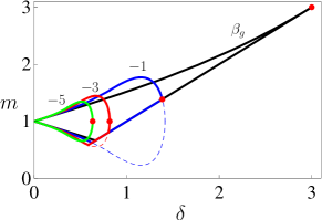
Figure 15: Average and width of the solution domain m𝑚m and δ𝛿\delta [Eq. (15)] as a function of β𝛽\beta. Solid line: stable branch. Dotted line: metastable branch.
Refer to caption
Refer to caption
Figure 16: Internal energy density u𝑢u and entropy density s𝑠s versus β𝛽\beta. Solid line: stable branch. Dotted line: metastable branch.

Finally, we record the interesting behavior of the minimum eigenvalue a=mδ𝑎𝑚𝛿a=m-\delta: see Fig. 17. For 2<β<22𝛽2-2<\beta<2, a𝑎a coincides with the origin (left border of the solution domain). This variable can be taken as an order parameter for both the second order phase transitions at β=2𝛽2\beta=-2 and at β+=2subscript𝛽2\beta_{+}=2. The 2subscript2\mathbb{Z}_{2} symmetry is broken for 2<β<22𝛽2-2<\beta<2. Notice, however, that the gravity critical point at βg=2/27subscript𝛽𝑔227\beta_{g}=-2/27 remains undetected by a𝑎a.

Refer to caption
Figure 17: Minimum eigenvalue a=mδ𝑎𝑚𝛿a=m-\delta versus β𝛽\beta. Solid line: stable branch. Dotted line: metastable branch.

Let us briefly comment on the fact that the analytic continuation of the solution at positive β𝛽\beta described in the previous subsection has not led us towards separable states. The eigenvalues remain of 𝒪(1/N)𝒪1𝑁{\cal O}\left(1/N\right) (and so does purity) even though the temperature can be (very) negative (as β𝛽\beta crosses 00). In order to find separable states we will have to look at the stable branch in the following subsection.

IV.2 Stable branch of separable states

In this section we will search the stable solution of the system at negative temperatures. As anticipated in Sec. II, from the definition (4) of the partition function one expects that, for any N𝑁N, as β𝛽\beta\rightarrow-\infty the system approaches the region of the phase space associated to separable states: here the purity is 𝒪(1)𝒪1{\cal O}\left(1\right) and the right scaling in Eqs. (4)-(5) is α=2𝛼2\alpha=2. In other words, by adopting the scaling N2superscript𝑁2N^{2} for the exponent of the partition function, we will explore the region β=𝒪(1/N)𝛽𝒪1𝑁\beta={\cal O}\left(1/N\right) of the scaling N3superscript𝑁3N^{3} introduced for positive temperatures. Notice that the critical point β=2/27𝛽227\beta=-2/27 for the solution at negative temperatures now reads β=(2/27)N𝛽227𝑁\beta=-(2/27)N and escapes to -\infty in the thermodynamic limit.

We will show that the solution (45), according to which all the eigenvalues are 𝒪(1/N)𝒪1𝑁{\cal O}\left(1/N\right), becomes metastable in the region of negative temperatures, and the distribution of the eigenvalues minimizing the free energy is such that one eigenvalue is 𝒪(1)𝒪1{\cal O}\left(1\right): this solution in the limit β𝛽\beta\rightarrow-\infty will correspond to the case of separable states. By following an approach similar to that adopted for positive temperatures, we will first look for the set of eigenvalues {λ1,,λN}subscript𝜆1subscript𝜆𝑁\{\lambda_{1},\ldots,\lambda_{N}\} satisfying the saddle point equations (9)-(10) with α=2𝛼2\alpha=2, getting as in Sec. III a continuous family of solutions. We will select among them the set maximizing (β<0𝛽0\beta<0) the free energy (8), with α=2𝛼2\alpha=2:

fN=i=1Nλi22N2β1i<jNln|λjλi|.subscript𝑓𝑁superscriptsubscript𝑖1𝑁superscriptsubscript𝜆𝑖22superscript𝑁2𝛽subscript1𝑖𝑗𝑁subscript𝜆𝑗subscript𝜆𝑖\displaystyle f_{N}=\sum_{i=1}^{N}\lambda_{i}^{2}-\frac{2}{N^{2}\beta}\sum_{1\leq i<j\leq N}\ln|\lambda_{j}-\lambda_{i}|. (82)

As emphasized at the beginning of this section, since we are approaching the limit β𝛽\beta\rightarrow-\infty the states occupying the largest volume in phase space are separable; we then define λN=μsubscript𝜆𝑁𝜇\lambda_{N}=\mu as the maximum eigenvalue and conjecture it to be of order of unity, whereas the other eigenvalues are 𝒪(1/N)𝒪1𝑁{\cal O}\left(1/N\right):

λN=μ=𝒪(1),1iN1λi=1μ.formulae-sequencesubscript𝜆𝑁𝜇𝒪1subscript1𝑖𝑁1subscript𝜆𝑖1𝜇\lambda_{N}=\mu={\cal O}\left(1\right),\quad\sum_{1\leq i\leq N-1}\lambda_{i}=1-\mu. (83)

From this it follows that we need to introduce the natural scaling only for the first N1𝑁1N-1 eigenvalues in order to solve the saddle point equations in the continuous limit and then estimate the thermodynamic quantities:

λisubscript𝜆𝑖\displaystyle\lambda_{i} =\displaystyle= (1μ)λ(ti)N1,1𝜇𝜆subscript𝑡𝑖𝑁1\displaystyle(1-\mu)\frac{\lambda(t_{i})}{N-1},
0<ti=iN11,i=1,,N1.formulae-sequence0subscript𝑡𝑖𝑖𝑁11for-all𝑖1𝑁1\displaystyle\quad 0<t_{i}=\frac{i}{N-1}\leq 1,\quad\forall i=1,\ldots,N-1.

In particular we will separately solve the saddle point equations (9)-(10), corresponding to the minimization of the exponent of the partition function with respect to the first N1𝑁1N-1 eigenvalues and the Lagrange multiplier ξ𝜉\xi, given, in the limit N𝑁N\to\infty, by

P0ρ¯(λ)dλλλiξ2(1μ)=0,𝑃superscriptsubscript0¯𝜌superscript𝜆𝑑superscript𝜆𝜆superscript𝜆𝑖𝜉21𝜇0\displaystyle P\int_{0}^{\infty}\frac{\bar{\rho}(\lambda^{\prime})d\lambda^{\prime}}{\lambda-\lambda^{\prime}}-i\frac{\xi}{2}(1-\mu)=0, (85)
with0λρ¯(λ)𝑑λ=1,withsuperscriptsubscript0𝜆¯𝜌𝜆differential-d𝜆1\displaystyle\quad\mathrm{with}\qquad\int_{0}^{\infty}\lambda\bar{\rho}(\lambda)d\lambda=1,

and we will then consider the condition deriving from the saddle point equation associated to μ𝜇\mu

2μβ+iξ=0.2𝜇𝛽𝑖𝜉02\mu\beta+i\xi=0. (86)

The function ρ¯¯𝜌\bar{\rho} introduced in (85) is the density of the eigenvalues associated to λ1,λN1subscript𝜆1subscript𝜆𝑁1\lambda_{1},\ldots\lambda_{N-1} in (IV.2) and has the same form (14) introduced for ρ(λ)𝜌𝜆\rho(\lambda) in the regime of positive temperatures. By the same change of variables introduced in Sec. III, Eqs. (15)-(16), the solution of the integral equations (85) can be expressed in terms of ϕ¯(x)=ρ¯(λ)δ¯italic-ϕ𝑥¯𝜌𝜆𝛿\bar{\phi}(x)=\bar{\rho}(\lambda)\delta:

ϕ¯(x)=1π1x2(12x(m1)δ).¯italic-ϕ𝑥1𝜋1superscript𝑥212𝑥𝑚1𝛿\bar{\phi}(x)=\frac{1}{\pi\sqrt{1-x^{2}}}\left(1-\frac{2x(m-1)}{\delta}\right). (87)

and the Lagrange multiplier is ξ=i4(m1)/(δ2(1μ))𝜉𝑖4𝑚1superscript𝛿21𝜇\xi=-i4(m-1)/(\delta^{2}(1-\mu)). The region of the parameter space (m,δ)𝑚𝛿(m,\delta) such that the density of eigenvalues ϕ¯¯italic-ϕ\bar{\phi} is nonnegative reads

max{δ, 1δ2}m1+δ2,𝛿1𝛿2𝑚1𝛿2\max\left\{\delta,\;1-\frac{\delta}{2}\right\}\leq m\leq 1+\frac{\delta}{2}, (88)

which is the same expression of the domain found for the range of positive temperatures (25) when β=0𝛽0\beta=0, namely Γ1±(δ,0)=1±δ/2superscriptsubscriptΓ1plus-or-minus𝛿0plus-or-minus1𝛿2\Gamma_{1}^{\pm}(\delta,0)=1\pm\delta/2 (see Fig. 18, which is the analog of Fig. 1). This is consistent with the change in temperature scaling from N3superscript𝑁3N^{3} in the case of positive temperatures to N2superscript𝑁2N^{2} in the case of negative temperatures: we are “zooming” into the region near β0𝛽superscript0\beta\rightarrow 0^{-} of the range of temperatures analyzed in paper1 and Sec. III. Summarizing, as could be expected from what we have shown for positive temperatures, the solution of the saddle point equations is a two parameter continuous family of solutions. We now have to determine the density of eigenvalues that maximizes the free energy of the system. From Eqs. (83) and (82) we get

fN=μ22N2β1i<jNln|λjλi|+𝒪(1N)subscript𝑓𝑁superscript𝜇22superscript𝑁2𝛽subscript1𝑖𝑗𝑁subscript𝜆𝑗subscript𝜆𝑖𝒪1𝑁f_{N}=\mu^{2}-\frac{2}{N^{2}\beta}\sum_{1\leq i<j\leq N}\ln|\lambda_{j}-\lambda_{i}|+{\cal O}\left(\frac{1}{N}\right) (89)

and by applying the scaling (IV.2)

fNsubscript𝑓𝑁\displaystyle f_{N} =\displaystyle= μ21βln(1μ)+fred(δ,m,β)superscript𝜇21𝛽1𝜇subscript𝑓red𝛿𝑚𝛽\displaystyle\mu^{2}-\frac{1}{\beta}\ln{(1-\mu)}+f_{\mathrm{red}}(\delta,m,\beta) (90)
+1βlnN+𝒪(lnNN)1𝛽𝑁𝒪𝑁𝑁\displaystyle+\frac{1}{\beta}\ln N+{\cal O}\left(\frac{\ln N}{N}\right)
=\displaystyle= f+1βlnN+𝒪(lnNN),𝑓1𝛽𝑁𝒪𝑁𝑁\displaystyle f+\frac{1}{\beta}\ln N+{\cal O}\left(\frac{\ln N}{N}\right),

where

f=limN(fN1βlnN)=μ21βln(1μ)+fred,𝑓subscript𝑁subscript𝑓𝑁1𝛽𝑁superscript𝜇21𝛽1𝜇subscript𝑓redf=\lim_{N\to\infty}\left(f_{N}-\frac{1}{\beta}\ln N\right)=\mu^{2}-\frac{1}{\beta}\ln{(1-\mu)}+f_{\mathrm{red}}, (91)

is the free energy density in the thermodynamic limit, and

fred(δ,m,β)subscript𝑓red𝛿𝑚𝛽\displaystyle f_{\mathrm{red}}(\delta,m,\beta) =\displaystyle= 1β11𝑑xϕ¯(x)11𝑑yϕ¯(y)ln(δ|xy|)1𝛽superscriptsubscript11differential-d𝑥¯italic-ϕ𝑥superscriptsubscript11differential-d𝑦¯italic-ϕ𝑦𝛿𝑥𝑦\displaystyle-\frac{1}{\beta}\int_{-1}^{1}\ dx\bar{\phi}(x)\int_{-1}^{1}\ dy\bar{\phi}(y)\ln(\delta|x-y|) (92)
=\displaystyle= 2(m1)2βδ21βln(δ2)2superscript𝑚12𝛽superscript𝛿21𝛽𝛿2\displaystyle\frac{2(m-1)^{2}}{\beta\delta^{2}}-\frac{1}{\beta}\ln\left(\frac{\delta}{2}\right)

is the reduced free energy density of the sea of eigenvalues.

It is easy to see that βfred(m,δ)𝛽subscript𝑓red𝑚𝛿\beta f_{\mathrm{red}}(m,\delta), has no stationary points, but only a global minimum βfred=1/2𝛽subscript𝑓red12\beta f_{\mathrm{red}}=1/2 at (δ,m)=(2,2)𝛿𝑚22(\delta,m)=(2,2), see arrow in Fig. 18; this point yields the Wishart distribution found at β=0𝛽0\beta=0 for the case of positive temperature (see also paper1 ):

ϕ¯(x)=1π1x1+x,ρ¯(λ)=12π4λλ,formulae-sequence¯italic-ϕ𝑥1𝜋1𝑥1𝑥¯𝜌𝜆12𝜋4𝜆𝜆\bar{\phi}(x)=\frac{1}{\pi}\sqrt{\frac{1-x}{1+x}},\quad\bar{\rho}(\lambda)=\frac{1}{2\pi}\sqrt{\frac{4-\lambda}{\lambda}}, (93)

where one should remember that the λ𝜆\lambda’s are also scaled by 1μ1𝜇1-\mu, see Eq. (IV.2).

Refer to caption
Figure 18: Contour plot of the reduced free energy βfred(δ,m)𝛽subscript𝑓red𝛿𝑚\beta f_{\mathrm{red}}(\delta,m) of the sea for negative temperatures. The arrow points at the minimum.
Refer to caption
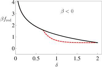
Figure 19: Reduced free energy βfred𝛽subscript𝑓red\beta f_{\mathrm{red}} on the boundary of the triangular domain in Fig. 18 for the case of negative temperatures. Solid line: upper boundary; dashed line: lower boundary.

We stress that this result is valid for all β<0𝛽0\beta<0. In order to check this solution one has to compute the free energy on the boundary of this domain, see Fig. 19 (which is the analog of Fig. 3). One gets that the free energy density is given by

f(μ,β)=μ21βln(1μ)+12β.𝑓𝜇𝛽superscript𝜇21𝛽1𝜇12𝛽\displaystyle f(\mu,\beta)=\mu^{2}-\frac{1}{\beta}\ln{(1-\mu)}+\frac{1}{2\beta}. (94)
Refer to caption
Figure 20: Evaporation of the eigenvalue μ=𝒪(1)𝜇𝒪1\mu={\cal O}\left(1\right) from the sea of eigenvalues 𝒪(1/N)𝒪1𝑁{\cal O}\left(1/N\right).

A new stationary solution, in which the largest isolated eigenvalue μ𝜇\mu becomes 𝒪(1)𝒪1{\cal O}\left(1\right), can be found by minimizing the free energy density and yields

μ(β)=12+121+2β,𝜇𝛽121212𝛽\mu(\beta)=\frac{1}{2}+\frac{1}{2}\sqrt{1+\frac{2}{\beta}}, (95)

being defined only for β<2𝛽2\beta<-2; this expression can also be obtained directly by the saddle point equation (86) corresponding to the isolated eigenvalue μ𝜇\mu. This eigenvalue, 𝒪(1)𝒪1{\cal O}\left(1\right), evaporates from the sea of eigenvalues 𝒪(1/N)𝒪1𝑁{\cal O}\left(1/N\right), as pictorially represented in Fig. 20. The isolated eigenvalue moves at a speed dμ/dβ=1/(2β4+2β3)𝑑𝜇𝑑𝛽12superscript𝛽42superscript𝛽3-d\mu/d\beta=1/(2\sqrt{\beta^{4}+2\beta^{3}}), which diverges at β=2𝛽2\beta=-2: another symptom of criticality. However, this new solution, when it appears at β=2𝛽2\beta=-2, is not the global minimum of βf𝛽𝑓\beta f: as we shall see it eventually becomes stable at a lower value of β𝛽\beta. We get for β<2𝛽2\beta<-2 (i.e. 0<μ<10𝜇10<\mu<1)

u𝑢\displaystyle u =\displaystyle= μ2=12+12β+121+2β,superscript𝜇21212𝛽1212𝛽\displaystyle\mu^{2}=\frac{1}{2}+\frac{1}{2\beta}+\frac{1}{2}\sqrt{1+\frac{2}{\beta}}, (96)
s𝑠\displaystyle s =\displaystyle= ln(1μ)12=ln(12121+2β)12,1𝜇12121212𝛽12\displaystyle\ln(1-\mu)-\frac{1}{2}=\ln\left(\frac{1}{2}-\frac{1}{2}\sqrt{1+\frac{2}{\beta}}\right)-\frac{1}{2}, (97)
βf𝛽𝑓\displaystyle\beta f =\displaystyle= βus=12μ2(1μ)ln(1μ)𝛽𝑢𝑠12𝜇21𝜇1𝜇\displaystyle\beta u-s=\frac{1-2\mu}{2(1-\mu)}-\ln{(1-\mu)} (98)
=\displaystyle= 1+β2+β21+2βln(12121+2β),1𝛽2𝛽212𝛽121212𝛽\displaystyle 1+\frac{\beta}{2}+\frac{\beta}{2}\sqrt{1+\frac{2}{\beta}}-\ln\left(\frac{1}{2}-\frac{1}{2}\sqrt{1+\frac{2}{\beta}}\right),
Refer to caption
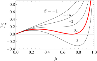
Figure 21: Reduced free energy as a function of μ𝜇\mu for different values of β(<0)annotated𝛽absent0\beta(<0). Notice the birth of a stationary point for β=2𝛽2\beta=-2 that becomes the global minimum for ββ𝛽subscript𝛽\beta\leq\beta_{-}.
Refer to caption
Refer to caption
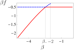
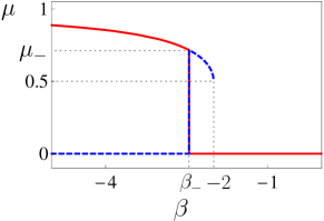
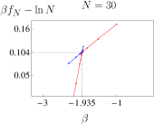
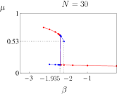
Figure 22: Free energy and maximum eigenvalue at negative temperatures. The two solutions are exchanged at β2.45541similar-to-or-equalssubscript𝛽2.45541\beta_{-}\simeq 2.45541, where there is a first order phase transition. Full line: solution of mimimal free energy; dashed line: solution of higher free energy.

We are now ready to unveil the presence of a first order phase transition in the system. In Fig. 21 we plot the free energy density as a function of μ𝜇\mu for different values of β𝛽\beta. For β>2𝛽2\beta>-2 there is a global minimum of βf𝛽𝑓\beta f at μ=0𝜇0\mu=0; μ𝜇\mu is still in the sea of the eigenvalues 𝒪(1/N)𝒪1𝑁{\cal O}\left(1/N\right) and the stable solution is given by the Wishart distribution (73) with the potentials (78) (remember that, in the zoomed scale considered here, βgsubscript𝛽𝑔\beta_{g} corresponds to the very large inverse temperature Nβg𝑁subscript𝛽𝑔N\beta_{g}). At β=2𝛽2\beta=-2 there appears a stationary point for the free energy density corresponding to μ=𝒪(1)𝜇𝒪1\mu={\cal O}\left(1\right) [see (95)]; notice however that βf𝛽𝑓\beta f at this point remains larger than its value at the global minimum, until β𝛽\beta reaches βsubscript𝛽\beta_{-}. Finally, for β<β𝛽subscript𝛽\beta<\beta_{-} the global minimum of βf𝛽𝑓\beta f moves to the right, to the solution containing μ=𝒪(1)𝜇𝒪1\mu={\cal O}\left(1\right). Summarizing, for β>β𝛽subscript𝛽\beta>\beta_{-} the solution of saddle point equations maximizing the free energy of the system is such that all eigenvalues are 𝒪(1/N)𝒪1𝑁{\cal O}\left(1/N\right), at β=2𝛽2\beta=-2 there appears a metastable solution for the system with one eigenvalue 𝒪(1)𝒪1{\cal O}\left(1\right), and for ββ𝛽subscript𝛽\beta\leq\beta_{-} this becomes the stable solution, that maximizes the free energy, whereas the distribution of the eigenvalues found in Sec. III becomes now metastable. The maximum eigenvalue is then a discontinuous function of the temperature at β=β𝛽subscript𝛽\beta=\beta_{-} and in the limit β𝛽\beta\rightarrow-\infty, μ𝜇\mu approaches 111: the state becomes separable. This critical temperature βsubscript𝛽\beta_{-} is the solution of the transcendental equation f(β,0)=f(β,μ)𝑓subscript𝛽0𝑓subscript𝛽subscript𝜇f(\beta_{-},0)=f(\beta_{-},\mu_{-}), that is

μ2(1μ)=ln(1μ),subscript𝜇21subscript𝜇1subscript𝜇\frac{\mu_{-}}{2(1-\mu_{-})}=-\ln(1-\mu_{-}), (99)

which yields

μ0.71533,β=12μ(1μ)2.45541.formulae-sequencesimilar-to-or-equalssubscript𝜇0.71533subscript𝛽12subscript𝜇1subscript𝜇similar-to-or-equals2.45541\mu_{-}\simeq 0.71533,\qquad\beta_{-}=-\frac{1}{2\mu_{-}(1-\mu_{-})}\simeq-2.45541. (100)

Therefore, the branch (97)-(98) is stable for β<β𝛽subscript𝛽\beta<\beta_{-} while it becomes metastable for β<β<2subscript𝛽𝛽2\beta_{-}<\beta<-2. On the other hand, the solution μ=0𝜇0\mu=0, corresponding to

u𝑢\displaystyle u =\displaystyle= μ2=0,superscript𝜇20\displaystyle\mu^{2}=0, (101)
s𝑠\displaystyle s =\displaystyle= β(uf)=12,𝛽𝑢𝑓12\displaystyle\beta(u-f)=-\frac{1}{2}, (102)
βf𝛽𝑓\displaystyle\beta f =\displaystyle= 12,12\displaystyle\frac{1}{2}, (103)

has a lower free energy for β<β<0subscript𝛽𝛽0\beta_{-}<\beta<0, and a higher one for β<β𝛽subscript𝛽\beta<\beta_{-}. See Fig. 22.

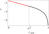
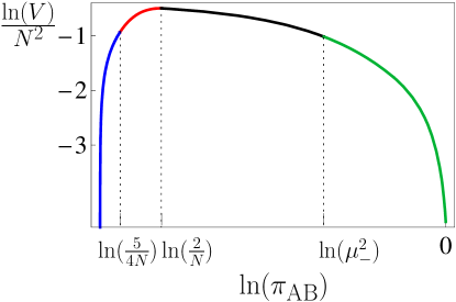
At βsubscript𝛽\beta_{-} there is a first order phase transition. At this fixed temperature the internal energy of the system goes from ur=0subscript𝑢𝑟0u_{r}=0 up to ul=μ20.5117subscript𝑢𝑙superscriptsubscript𝜇2similar-to-or-equals0.5117u_{l}=\mu_{-}^{2}\simeq 0.5117, while the entropy goes from sr=1/2subscript𝑠𝑟12s_{r}=-1/2 down to sl=1/2+ln(1μ)1.75643subscript𝑠𝑙121subscript𝜇similar-to-or-equals1.75643s_{l}=-1/2+\ln(1-\mu_{-})\simeq-1.75643. One gets Δs/Δu=βΔ𝑠Δ𝑢subscript𝛽\Delta s/\Delta u=\beta_{-}. Therefore, the entropy density as a function of the internal energy density reads

s(u)={βu12,0<u<μ2,ln(1u)12,μ2u<1.𝑠𝑢casessubscript𝛽𝑢120𝑢superscriptsubscript𝜇2otherwiseotherwise1𝑢12superscriptsubscript𝜇2𝑢1s(u)=\begin{cases}\beta_{-}u-\frac{1}{2},&0<u<\mu_{-}^{2},\\ \\ \ln(1-\sqrt{u})-\frac{1}{2},&\mu_{-}^{2}\leq u<1.\end{cases} (104)

It is continuous together with its first derivative at u=μ2𝑢superscriptsubscript𝜇2u=\mu_{-}^{2}, while its second derivative is discontinuous. Notice that Δu=Δs/βΔ𝑢Δ𝑠subscript𝛽\Delta u=\Delta s/\beta_{-} is the specific latent heat of the evaporation of the largest eigenvalue from the sea of the eigenvalues, from 𝒪(1/N)𝒪1𝑁{\cal O}\left(1/N\right) up to μsubscript𝜇\mu_{-}.

A few words of interpretation are necessary. As we have seen, it has been necessary to follow the stable branch of the solution in order to obtain separable states at negative temperatures. The analytic continuation of the stable solution for positive temperatures would yield an unstable branch in which all eigenvalues remain 𝒪(1/N)𝒪1𝑁{\cal O}\left(1/N\right). By contrast, the new stable solution consists in a sea of N1𝑁1N-1 eigenvalues 𝒪(1/N)𝒪1𝑁{\cal O}\left(1/N\right) plus one isolated eigenvalue 𝒪(1)𝒪1{\cal O}\left(1\right).

Let us discuss this result in terms of purity, like at the end of Sec. III (we stress again that β𝛽\beta is a Lagrange multiplier that fixes the value of the purity of the reduced density matrix of our N2superscript𝑁2N^{2}-dimensional system). Assume that we pick a given isopurity manifold in the original Hilbert space, defined by a given finite value πABsubscript𝜋𝐴𝐵\pi_{AB} of purity. If we randomly select a vector belonging to this isopurity manifold, its reduced density matrix (for the fixed bipartition) will have one finite eigenvalue μπABsimilar-to-or-equals𝜇subscript𝜋𝐴𝐵\mu\simeq\sqrt{\pi_{AB}} and many small eigenvalues 𝒪(1/N)𝒪1𝑁{\cal O}\left(1/N\right) (yielding a correction 𝒪(1/N)𝒪1𝑁{\cal O}\left(1/N\right) to purity). In this sense, the quantum state is largely separable. The probability of finding in the afore-mentioned manifold a vector whose reduced density matrix has, say, two (or more) finite eigenvalues μ1subscript𝜇1\mu_{1} and μ2subscript𝜇2\mu_{2} (such that μ12+μ22πABsimilar-to-or-equalssuperscriptsubscript𝜇12superscriptsubscript𝜇22subscript𝜋𝐴𝐵\mu_{1}^{2}+\mu_{2}^{2}\simeq\pi_{AB}, modulo corrections 𝒪(1/N)𝒪1𝑁{\cal O}\left(1/N\right)) is vanishingly small. By contrast, remember (from the results of Sec. III) that if the isopurity manifold is characterized by a very small value 𝒪(1/N)𝒪1𝑁{\cal O}\left(1/N\right) of purity, the eigenvalues of a randomly chosen vector on the manifold are all 𝒪(1/N)𝒪1𝑁{\cal O}\left(1/N\right) (being distributed according to the semicircle or Wishart, depending on the precise value of purity, as seen in Sec. III). This is the significance of the statistical mechanical approach adopted in this article. We will come back to this point in Sec. VI.

V Finite size systems

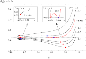
The results of the previous section refer to N𝑁N\to\infty. In order to understand how finite-N𝑁N corrections affect our conclusions we have numerically minimized the free energy for various temperatures. The two phases of the system discussed in the previous section correspond to the two solutions obtained by minimizing the free energy βfN𝛽subscript𝑓𝑁\beta f_{N} (82) on the N𝑁N dimensional simplex of the normalized eigenvalues. Indeed, we have numerically proved that βfN(β)𝛽subscript𝑓𝑁𝛽\beta f_{N}(\beta) presents two local minima at negative temperatures: for 0β>β(N)0𝛽superscriptsubscript𝛽𝑁0\geq\beta>\beta_{-}^{(N)} the minimum giving the lower value of βfN(β)𝛽subscript𝑓𝑁𝛽\beta f_{N}(\beta) corresponds to the distribution of eigenvalues (45), found in the last section; the other minimum is reached when the highest eigenvalue is 𝒪(1)𝒪1{\cal O}\left(1\right). The point β=β(N)𝛽superscriptsubscript𝛽𝑁\beta=\beta_{-}^{(N)} is a crossing point for these two solutions, and for ββ(N)𝛽superscriptsubscript𝛽𝑁\beta\leq\beta_{-}^{(N)} these two solutions are inverted, see Fig. 22 (and 21). Summarizing, there exists a negative temperature at which the system undergoes a first-order phase transition, from typical to separable states.

The first thing to notice is that qualitatively the phase transition remains of first order even for finite N𝑁N. The second is that the finite N𝑁N corrections are quite relevant for the location of the phase transition and the value of the maximum eigenvalue as a function of β𝛽\beta. For example, for N=30𝑁30N=30, the negative critical temperature β(30)=1.935superscriptsubscript𝛽301.935\beta_{-}^{(30)}=-1.935 instead of 2.4552.455-2.455. This is evinced from Fig. 23, which is the finite size version of Fig. 22. This can be understood, as the corrections to f(μ)𝑓𝜇f(\mu) around μ=0𝜇0\mu=0 are quite large. In the limit μ=1/N𝜇1𝑁\mu=1/N there is a hard wall for the maximum eigenvalue μ𝜇\mu, as the condition iλi=1subscript𝑖subscript𝜆𝑖1\sum_{i}\lambda_{i}=1 cannot be satisfied if μ<1/N𝜇1𝑁\mu<1/N. It is therefore likely that all sorts of large corrections occur as μ𝜇\mu tends to 1/N1𝑁1/N, probably yielding an effective size to the corrections which is a lower power of 1/N1𝑁1/N (or even possibly 1/lnN1𝑁1/\ln N). The limits μ0𝜇0\mu\to 0 and N𝑁N\to\infty do not commute.

Refer to caption
Refer to caption
Figure 23: Finite N𝑁N version of Fig. 22. Free energy and maximum eigenvalue in the saddle point approximation as function of β𝛽\beta at N=30𝑁30N=30. The local minimum is in blue, the global one in red. The two minima swap stability at β=1.935𝛽1.935\beta=-1.935. Notice the birth of the new local minimum at β=1.8𝛽1.8\beta=-1.8 (for N=𝑁N=\infty this takes place at β=2𝛽2\beta=-2) and the exchange of stability at β=1.93𝛽1.93\beta=-1.93 (for N=𝑁N=\infty, β=2.45𝛽2.45\beta=-2.45).
Refer to caption
Figure 24: Finite N𝑁N version of Fig. 21. βfNlnN𝛽subscript𝑓𝑁𝑁\beta f_{N}-\ln N as a function of the maximum eigenvalue μ𝜇\mu, obtained by numerical minimization over the remaining N1𝑁1N-1 eigenvalues for various β𝛽\beta. Observe the formation of a new minimum and the exchange of stability, although the critical values of β𝛽\beta at which these phenomena occur differ from the theoretical ones, due to large finite N𝑁N corrections. However, it is clear that at small μ𝜇\mu, 1/N1𝑁1/N corrections tend to increase the value of βfN𝛽subscript𝑓𝑁\beta f_{N}, making the critical value βsubscript𝛽\beta_{-} move towards 0, as observed in the numerics.
Refer to caption
Figure 25: Value of β𝛽\beta at which the second minimum is born as a function of N𝑁N. The solid curve is a best fit returning βμ(N)=1.9976.04/Nsuperscriptsubscript𝛽𝜇𝑁1.9976.04𝑁\beta_{\mu}^{(N)}=-1.997-6.04/N. The asymptotic value should be 2 and is in good agreement with the constant of the fit.
Refer to caption
Figure 26: Maximal eigenvalue in the saddle point approximation as function of β𝛽\beta. The points are the result of a numerical evaluation for N=40𝑁40N=40, while the full line is the expression in Eq. (105).

To further explore this effect we minimized βfN𝛽subscript𝑓𝑁\beta f_{N} with respect to λ1,,λN1subscript𝜆1subscript𝜆𝑁1\lambda_{1},\ldots,\lambda_{N-1}, for fixed values of the largest eigenvalue λN=μsubscript𝜆𝑁𝜇\lambda_{N}=\mu and for different temperatures. The results for N=30𝑁30N=30 are shown in Fig. 24. One can see that between β=1.8𝛽1.8\beta=-1.8 and β=2.5𝛽2.5\beta=-2.5 there is a competition between two well defined local minima, corresponding to the two solutions discussed above. At β=β(30)=1.935𝛽superscriptsubscript𝛽301.935\beta=\beta_{-}^{(30)}=-1.935 their free energies are equal. For higher β𝛽\beta the global minimum corresponds to the solution (45), whereas on the other side of β(30)superscriptsubscript𝛽30\beta_{-}^{(30)} the solution with μ=𝒪(1)𝜇𝒪1\mu={\cal O}\left(1\right) minimizes βfN𝛽subscript𝑓𝑁\beta f_{N}. Similar corrections are observed for the value of β=βμ(N)𝛽superscriptsubscript𝛽𝜇𝑁\beta=\beta_{\mu}^{(N)} at which the second minimum is born. See Fig. 25.

We have seen that for β>β𝛽subscript𝛽\beta>\beta_{-} the stable solution has no detached eigenvalue. By taking into account the scaling ββ/N𝛽𝛽𝑁\beta\to\beta/N we get that the solution is given by the very first part of the gravity branch (78). In particular, the maximum eigenvalue is given by b/N=(m+δ)/N=2δ/N𝑏𝑁𝑚𝛿𝑁2𝛿𝑁b/N=(m+\delta)/N=2\delta/N. On the other hand for β<β𝛽subscript𝛽\beta<\beta_{-} the maximum eigenvalue is given by (95). Therefore, we get

μ={12+121+2β,ββ,2Nδ(β/N),β<β<0,𝜇cases121212𝛽𝛽subscript𝛽otherwiseotherwise2𝑁𝛿𝛽𝑁subscript𝛽𝛽0\displaystyle\mu=\begin{cases}\frac{1}{2}+\frac{1}{2}\sqrt{1+\frac{2}{\beta}},&\beta\leq\beta_{-},\\ \\ \frac{2}{N}\delta(\beta/N),&\beta_{-}<\beta<0,\end{cases} (105)

with δ(β)𝛿𝛽\delta(\beta) given by (46)-(48). The numerical results for N=40𝑁40N=40 are compared with the expressions in Eq. (105) in Fig. 26. The agreement is excellent.

The corresponding free energy follows from (98) and (78) with the appropriate scaling

βf={1+β2+β21+2βln(12121+2β),ββ,1149δ(β/N)+9δ(β/N)2lnδ(β/N)2,β<β<0.𝛽𝑓cases1𝛽2𝛽212𝛽121212𝛽𝛽subscript𝛽otherwiseotherwise1149𝛿𝛽𝑁9𝛿superscript𝛽𝑁2𝛿𝛽𝑁2subscript𝛽𝛽0\displaystyle\beta f=\begin{cases}1+\frac{\beta}{2}+\frac{\beta}{2}\sqrt{1+\frac{2}{\beta}}-\ln\left(\frac{1}{2}-\frac{1}{2}\sqrt{1+\frac{2}{\beta}}\right),&\beta\leq\beta_{-},\\ \\ \frac{11}{4}-\frac{9}{\delta(\beta/N)}+\frac{9}{\delta(\beta/N)^{2}}-\ln\frac{\delta(\beta/N)}{2},&\beta_{-}<\beta<0.\end{cases} (106)

Notice that in order to have a finite size scaling of the critical temperature β(N)superscriptsubscript𝛽𝑁\beta_{-}^{(N)} one should take into account 𝒪(1/N)𝒪1𝑁{\cal O}\left(1/N\right) corrections to the expression of βf𝛽𝑓\beta f and then evaluate the intersection between the two branches, but this analysis goes beyond our scope.

VI Overview

Let us summarize the main results obtained in this article in more intuitive terms, by focusing on those quantities that are more directly related to physical intuition. In the statistical mechanical approach adopted in this article, the temperature plays the usual role of a Lagrange multiplier, whose only task is to fix the value of energy (purity in our case). A given value of β𝛽\beta determines a set of vectors in the projective Hilbert space whose reduced density matrices have a given purity (isopurity manifold of quantum states). The distribution of the eigenvalues of (the reduced density matrices associated to) these vectors is that investigated in this article and yields information on the separability (entanglement) of these quantum states. The distribution of eigenvalues is the most probable one mehta (in the same way as the Maxwell distribution of molecular velocities is the most probable one at a given temperature). Let us therefore abandon temperature in the following and fully adopt purity as our physical quantity.

Entropy counts the number of states with a given value of purity and is in this sense proportional to the logarithm of the volume in the projective Hilbert space. The explicit expressions of the entropy density s𝑠s, which is the logarithm of the volume of the isopurity manifold, as a function of the purity πABsubscript𝜋𝐴𝐵\pi_{AB} of the state vectors in that volume, can be read directly from Eqs. (58) and (104) by taking into account the correct scaling:

s(πAB)={12ln(NπAB1)14,1N<πAB54N,ln(3294NπAB)94+52(3294NπAB)34(3294NπAB)2,54N<πAB2N,βπAB12,2N<πABμ2,ln(1πAB)12,μ2<πAB<1,𝑠subscript𝜋𝐴𝐵cases12𝑁subscript𝜋𝐴𝐵1141𝑁subscript𝜋𝐴𝐵54𝑁otherwiseotherwise3294𝑁subscript𝜋𝐴𝐵94523294𝑁subscript𝜋𝐴𝐵34superscript3294𝑁subscript𝜋𝐴𝐵254𝑁subscript𝜋𝐴𝐵2𝑁otherwiseotherwisesubscript𝛽subscript𝜋𝐴𝐵122𝑁subscript𝜋𝐴𝐵superscriptsubscript𝜇2otherwiseotherwise1subscript𝜋𝐴𝐵12superscriptsubscript𝜇2subscript𝜋𝐴𝐵1\displaystyle s(\pi_{AB})=\begin{cases}\frac{1}{2}\ln(N\pi_{AB}-1)-\frac{1}{4},&\frac{1}{N}<\pi_{AB}\leq\frac{5}{4N},\\ \\ \ln\left(\frac{3}{2}-\sqrt{\frac{9}{4}-N\pi_{AB}}\right)-\frac{9}{4}+\frac{5}{2\left(\frac{3}{2}-\sqrt{\frac{9}{4}-N\pi_{AB}}\right)}-\frac{3}{4\left(\frac{3}{2}-\sqrt{\frac{9}{4}-N\pi_{AB}}\right)^{2}},&\frac{5}{4N}<\pi_{AB}\leq\frac{2}{N},\\ \\ \beta_{-}\pi_{AB}-\frac{1}{2},&\frac{2}{N}<\pi_{AB}\leq\mu_{-}^{2},\\ \\ \ln\left(1-\sqrt{\pi_{AB}}\right)-\frac{1}{2},&\mu_{-}^{2}<\pi_{AB}<1,\end{cases} (107)
Refer to caption
Refer to caption
Figure 27: Entropy density s𝑠s versus internal energy density u𝑢u. Notice that the unit on the abscissae is 1/N1𝑁1/N in the left panel.

with μ20.512similar-to-or-equalssuperscriptsubscript𝜇20.512\mu_{-}^{2}\simeq 0.512 and β2.455similar-to-or-equalssubscript𝛽2.455\beta_{-}\simeq-2.455 given by (99)-(100). The plot of s𝑠s vs πABsubscript𝜋𝐴𝐵\pi_{AB} in the two regions πAB=𝒪(1/N)subscript𝜋𝐴𝐵𝒪1𝑁\pi_{AB}={\cal O}\left(1/N\right) and πAB=𝒪(1)subscript𝜋𝐴𝐵𝒪1\pi_{AB}={\cal O}\left(1\right) is shown in Fig. 27. By exponentiating the expression (107) we get the volume V=exp(N2s)𝑉superscript𝑁2𝑠V=\exp{(N^{2}s)} (i.e. the probability) of the isopurity manifolds

V(πAB){eN24(NπAB1)N2/2,1N<πAB54N,(3294NπAB)N2exp[N2(94+52(3294NπAB)34(3294NπAB)2)],54N<πAB2N,exp[N2(βπAB12)],2N<πABμ2,eN22(1πAB)N2,μ2<πAB<1.proportional-to𝑉subscript𝜋𝐴𝐵casessuperscript𝑒superscript𝑁24superscript𝑁subscript𝜋𝐴𝐵1superscript𝑁221𝑁subscript𝜋𝐴𝐵54𝑁otherwiseotherwisesuperscript3294𝑁subscript𝜋𝐴𝐵superscript𝑁2superscript𝑁294523294𝑁subscript𝜋𝐴𝐵34superscript3294𝑁subscript𝜋𝐴𝐵254𝑁subscript𝜋𝐴𝐵2𝑁otherwiseotherwisesuperscript𝑁2subscript𝛽subscript𝜋𝐴𝐵122𝑁subscript𝜋𝐴𝐵superscriptsubscript𝜇2otherwiseotherwisesuperscript𝑒superscript𝑁22superscript1subscript𝜋𝐴𝐵superscript𝑁2superscriptsubscript𝜇2subscript𝜋𝐴𝐵1\displaystyle V(\pi_{AB})\propto\begin{cases}e^{-\frac{N^{2}}{4}}(N\pi_{AB}-1)^{N^{2}/2},&\frac{1}{N}<\pi_{AB}\leq\frac{5}{4N},\\ \\ \left(\frac{3}{2}-\sqrt{\frac{9}{4}-N\pi_{AB}}\right)^{N^{2}}\exp\left[N^{2}\left(-\frac{9}{4}+\frac{5}{2\left(\frac{3}{2}-\sqrt{\frac{9}{4}-N\pi_{AB}}\right)}-\frac{3}{4\left(\frac{3}{2}-\sqrt{\frac{9}{4}-N\pi_{AB}}\right)^{2}}\right)\right],&\frac{5}{4N}<\pi_{AB}\leq\frac{2}{N},\\ \\ \exp\left[N^{2}\left(\beta_{-}\pi_{AB}-\frac{1}{2}\right)\right],&\frac{2}{N}<\pi_{AB}\leq\mu_{-}^{2},\\ \\ e^{-\frac{N^{2}}{2}}\left(1-\sqrt{\pi_{AB}}\right)^{N^{2}},&\mu_{-}^{2}<\pi_{AB}<1.\end{cases} (108)
Refer to caption
Figure 28: Volume V=exp(N2s)𝑉superscript𝑁2𝑠V=\exp(N^{2}s) of the isopurity manifolds versus their purity πABsubscript𝜋𝐴𝐵\pi_{AB} for N=50𝑁50N=50.
Refer to caption
Figure 29: Minimum eigenvalues as a function of πABsubscript𝜋𝐴𝐵\pi_{AB}. At πAB=5/4Nsubscript𝜋𝐴𝐵54𝑁\pi_{AB}=5/4N the gap vanishes.
Refer to caption
Refer to caption
Figure 30: Maximum eigenvalue as a function of πABsubscript𝜋𝐴𝐵\pi_{AB}.

This is plotted in Fig. 28 for N=50𝑁50N=50. The presence of discontinuities in some derivatives of entropy detects the two phase transitions. At πAB=5/4Nsubscript𝜋𝐴𝐵54𝑁\pi_{AB}=5/4N there is a second order phase transition signaled by a discontinuity in the third derivative. Indeed, in general, if s,u𝑠𝑢s,u and T𝑇T are entropy, energy and temperature, respectively, and C=du/dT𝐶𝑑𝑢𝑑𝑇C=du/dT is the specific heat, one gets ds/du=β=1/T𝑑𝑠𝑑𝑢𝛽1𝑇ds/du=\beta=1/T and d2s/du2=1/(T2C)=(1/T3)(ds/dT)1.superscript𝑑2𝑠𝑑superscript𝑢21superscript𝑇2𝐶1superscript𝑇3superscript𝑑𝑠𝑑𝑇1d^{2}s/du^{2}=-1/(T^{2}C)=-(1/T^{3})(ds/dT)^{-1}. Discontinuities of the n𝑛nth derivative of ds/dT𝑑𝑠𝑑𝑇ds/dT translate therefore in discontinuities of the (n+1)𝑛1(n+1)-th derivative of ds/du𝑑𝑠𝑑𝑢ds/du. The first order phase transition, which takes place between πAB=2/Nsubscript𝜋𝐴𝐵2𝑁\pi_{AB}=2/N and πAB=μ20.512subscript𝜋𝐴𝐵superscriptsubscript𝜇2similar-to-or-equals0.512\pi_{AB}=\mu_{-}^{2}\simeq 0.512 is signaled by discontinuities in the second derivative of the entropy at those points. Observe that entropy is unbounded from below: at both endpoints of the range of purity, πAB=1/Nsubscript𝜋𝐴𝐵1𝑁\pi_{AB}=1/N (maximally entangled states) and πAB=1subscript𝜋𝐴𝐵1\pi_{AB}=1 (separable states), when the isopurity manifold shrinks to a vanishing volume in the original Hilbert space, the entropy, being the logarithm of this volume, diverges, and the number of vector states goes to zero (compared to the number of typical vector states). See Fig.  28.

The presence of the phase transitions can be easily read out from the behavior of the distribution of the Schmidt coefficients, i.e. the eigenvalues of the reduced density matrix ρAsubscript𝜌𝐴\rho_{A} of one subsystem. From Eq. (56) we get the expression of the minimum eigenvalue λmin=a=mδsubscript𝜆min𝑎𝑚𝛿\lambda_{\mathrm{min}}=a=m-\delta as a function of πABsubscript𝜋𝐴𝐵\pi_{AB}

λmin={1N(12NπAB1),1N<πAB54N,0,54N<πAB1.subscript𝜆mincases1𝑁12𝑁subscript𝜋𝐴𝐵11𝑁subscript𝜋𝐴𝐵54𝑁otherwiseotherwise054𝑁subscript𝜋𝐴𝐵1\displaystyle\lambda_{\mathrm{min}}=\begin{cases}\frac{1}{N}\left(1-2\sqrt{N\pi_{AB}-1}\right),&\frac{1}{N}<\pi_{AB}\leq\frac{5}{4N},\\ \\ 0,&\frac{5}{4N}<\pi_{AB}\leq 1.\end{cases} (109)

which is shown in Fig. 29. The second order phase transition at πAB=5/4Nsubscript𝜋𝐴𝐵54𝑁\pi_{AB}=5/4N, associated to a 2subscript2{\mathbb{Z}}_{2} symmetry breaking, is detected by a vanishing gap. On the other hand, the maximum eigenvalue λmaxsubscript𝜆max\lambda_{\mathrm{max}} coincides with the upper edge of the sea of eigenvalues b=m+δ𝑏𝑚𝛿b=m+\delta, as given by (56), until it evaporates according to Eq. (96). Thus,

λmax={1N(1+2NπAB1),1N<πAB54N,2N(3294NπAB),54N<πAB2NπAB,2N<πAB<1,subscript𝜆maxcases1𝑁12𝑁subscript𝜋𝐴𝐵11𝑁subscript𝜋𝐴𝐵54𝑁otherwiseotherwise2𝑁3294𝑁subscript𝜋𝐴𝐵54𝑁subscript𝜋𝐴𝐵2𝑁otherwiseotherwisesubscript𝜋𝐴𝐵2𝑁subscript𝜋𝐴𝐵1\displaystyle\lambda_{\mathrm{max}}=\begin{cases}\frac{1}{N}\left(1+2\sqrt{N\pi_{AB}-1}\right),&\frac{1}{N}<\pi_{AB}\leq\frac{5}{4N},\\ \\ \frac{2}{N}\left(3-2\sqrt{\frac{9}{4}-N\pi_{AB}}\right),&\frac{5}{4N}<\pi_{AB}\leq\frac{2}{N}\\ \\ \sqrt{\pi_{AB}},&\frac{2}{N}<\pi_{AB}<1,\end{cases} (110)
Refer to caption
Refer to caption
Refer to caption
Figure 31: Summary (stable branch): profiles of the eigenvalue density for 1πAB54N1subscript𝜋𝐴𝐵54𝑁1\leq\pi_{AB}\leq\frac{5}{4N}, 54NπAB2N54𝑁subscript𝜋𝐴𝐵2𝑁\frac{5}{4N}\leq\pi_{AB}\leq\frac{2}{N}, and 2NπAB12𝑁subscript𝜋𝐴𝐵1\frac{2}{N}\leq\pi_{AB}\leq 1.
Refer to caption
Figure 32: Overview of the “evolution” of the eigenvalue densities as a function of purity (1/NπAB1)1𝑁subscript𝜋𝐴𝐵1(1/N\leq\pi_{AB}\leq 1). The straight segment represents the stable branch: the distribution starts as a delta function, evolves into a semicircle, undergoes a second-order phase transition at πAB=5/4Nsubscript𝜋𝐴𝐵54𝑁\pi_{AB}=5/4N (2subscript2{\mathbb{Z}}_{2} symmetry breaking), becomes Wishart and undergoes a first-order phase transition between 2/NπAB0.51172𝑁subscript𝜋𝐴𝐵0.51172/N\leq\pi_{AB}\leq 0.5117, during which one eigenvalue evaporates from the sea of the others 𝒪(1/N)𝒪1𝑁{\cal O}\left(1/N\right) and becomes 𝒪(1)𝒪1{\cal O}\left(1\right). A metastable branch is born at πAB=2/Nsubscript𝜋𝐴𝐵2𝑁\pi_{AB}=2/N: it starts as Wishart, undergoes a second-order phase transition at πAB=9/4Nsubscript𝜋𝐴𝐵94𝑁\pi_{AB}=9/4N (2-D gravity), develops a singularity at its right edge through a second order phase transition at πAB=9/4Nsubscript𝜋𝐴𝐵94𝑁\pi_{AB}=9/4N, then its support starts decreasing, undergoes a second-order phase transition at πAB=7/4Nsubscript𝜋𝐴𝐵74𝑁\pi_{AB}=7/4N (2subscript2{\mathbb{Z}}_{2} symmetry restoration) and eventually becomes sharply peaked (with two singularities). The diamonds indicate the three second order phase transitions.

as shown in Fig. 30.

In the different phases the distribution of the eigenvalues of ρAsubscript𝜌𝐴\rho_{A} have very different profiles. See Fig. 31. While for 1πAB54N1subscript𝜋𝐴𝐵54𝑁1\leq\pi_{AB}\leq\frac{5}{4N} the eigenvalues (all 𝒪(1/N)𝒪1𝑁{\cal O}\left(1/N\right)) follow Wigner’s semicircle law, they become distributed according to Wishart for larger purities, 54NπAB2N54𝑁subscript𝜋𝐴𝐵2𝑁\frac{5}{4N}\leq\pi_{AB}\leq\frac{2}{N}, across the second order phase transition. This is a first signature of separability: some eigenvalues vanish and the Schmidt rank decreases. For even larger values of purity, 2NπAB12𝑁subscript𝜋𝐴𝐵1\frac{2}{N}\leq\pi_{AB}\leq 1, across the first order phase transition, one eigenvalue evaporates, leaving the sea of the other eigenvalues 𝒪(1/N)𝒪1𝑁{\cal O}\left(1/N\right) and becoming 𝒪(1)𝒪1{\cal O}\left(1\right). This is the signature of factorization, fully attained when the eigenvalue becomes 111 at πAB=1subscript𝜋𝐴𝐵1\pi_{AB}=1.

We tried to give an overview of the phenomenology of these phase transitions in Fig. 32, where we also showed the presence of the metastable branches discussed in Sec. IV. The global picture is both rich and involved and it would not be surprising if additional features would be unveiled by future investigation.

VII Conclusions

We have obtained a complete characterization of the statistical features of the bipartite entanglement of a large quantum system in a pure state. The global picture is interesting as several locally stable solutions exchange stabilities. On the stable branch (solutions of minimal free energy) there is a second order phase transition, associated to a 2subscript2{\mathbb{Z}}_{2} symmetry breaking, and related to the vanishing of some Schmidt coefficients (eigenvalues of the reduced density matrix of one subsystem), followed by a first order phase transition, associated to the evaporation of the largest eigenvalue from the sea of the others.

In the different phases the distribution of the Schmidt coefficients have very different profiles. While for large β𝛽\beta (small purity) the eigenvalues (all 𝒪(1/N)𝒪1𝑁{\cal O}\left(1/N\right)) follow Wigner’s semicircle law, they become distributed according to Wishart for smaller β𝛽\beta and larger purity, across the first transition. For even smaller (and eventually negative) values of β𝛽\beta, when purity becomes finite, across the second phase transition, one eigenvalue evaporates, leaving the sea of the other eigenvalues 𝒪(1/N)𝒪1𝑁{\cal O}\left(1/N\right) and becoming 𝒪(1)𝒪1{\cal O}\left(1\right). This is the signature of separability, this eigenvalue being associated with the emergence of factorization in the wave function (given the bipartition). This intepretation is suggestive and hints at a profound modification of the distribution of the eigenvalues as β𝛽\beta, and therefore purity, are changed. Remember that β𝛽\beta, viewed as a Lagrange multiplier in this statistical mechanical approach, localizes the measure on set of states with a given entanglement (isopurity manifolds Kus01 ).

It would be of great interest to understand whether the phase transitions survive even in the multipartite entanglement scenario, if one views the distribution of purity (over all balanced bipartitions) as a characterization of the global entanglement of the many-body wave function of the quantum system mmes . This description of multipartite entanglement displays the symptoms of frustration frust , catapulting the problem into one of the most fascinating arenas of modern statistical mechanics parisi .

While we were completing this work a paper appeared in which an aspect of this problem is discussed, although with a different emphasis Majumdar09 . In order to connect our results to those in Majumdar09 , notice that the probability distribution of the purity P(u)𝑃𝑢P(u) is proportional to the volume of the isopurity manifold and therefore

lnP(u)N2s(u),similar-to-or-equals𝑃𝑢superscript𝑁2𝑠𝑢\ln P(u)\simeq N^{2}s(u), (111)

where s𝑠s is the entropy and NπAB=u𝑁delimited-⟨⟩subscript𝜋𝐴𝐵𝑢N\langle\pi_{AB}\rangle=u is the internal energy. See Eq. (108).

VIII Acknowledgements

This work is partly supported by the European Union through the Integrated Project EuroSQIP.

References

  • (1) M.A. Nielsen and I.L. Chuang, Quantum Computation and Quantum Information (Cambridge University Press, Cambridge, 2000).
  • (2) G. Benenti, G. Casati and G. Strini, Principles of quantum computation and information, Volume I: Basic concepts (World Scientific, Singapore, 2004).
  • (3) L. Amico, R. Fazio, A. Osterloh and V. Vedral, Rev. Mod. Phys. 80, 517 (2008).
  • (4) R. Horodecki, P. Horodecki, M. Horodecki and K. Horodecki, Rev. Mod. Phys. 81, 865 (2009).
  • (5) W. K. Wootters, Quantum Inf. and Comp., 1, 27 (2001).
  • (6) C. H. Bennett, D. P. DiVincenzo, J. A. Smolin and W. K. Wootters, Phys. Rev. A 54 3824 (1996).
  • (7) V. Coffman, J. Kundu and W. K. Wootters, Phys. Rev. A 61, 052306 (2000); A. Wong and N. Christensen, Phys. Rev. A 63, 044301 (2001); D. Bruss, J. Math. Phys. 43, 4237 (2002); D.A. Meyer and N.R. Wallach, J. Math. Phys. 43, 4273 (2002); M. Jakob and J. Bergou, Phys. Rev. A 76 052107 (2007).
  • (8) P. Facchi, G. Florio, G. Parisi and S. Pascazio, Phys. Rev. A 77, 060304(R) (2008).
  • (9) P. Facchi, U. Marzolino, G. Parisi, S. Pascazio and A. Scardicchio, Phys. Rev. Lett. 101 050502 (2008).
  • (10) E. Lubkin, J. Math. Phys. 19, 1028 (1978); S. Lloyd and H. Pagels, Ann. Phys., NY, 188, 186 (1988); K Życzkowski and H.-J. Sommers, J. Phys. A 34, 7111 (2001); A. J. Scott and C. M. Caves, J. Phys. A: Math. Gen. 36, 9553 (2003).
  • (11) D.N. Page, Phys. Rev. Lett. 71, 1291 (1993).
  • (12) M. L. Mehta, Random Matrices (Elsevier Academic Press, San Diego, 2004).
  • (13) O. Giraud, J. Phys. A: Math. Theor. 40 (2007) 2793.
  • (14) F. G. Tricomi, Integral Equations (Cambridge University Press, Cambridge, 1957).
  • (15) P. Di Francesco, P. H. Ginsparg and J. Zinn-Justin, Phys. Rept.  254, 1 (1995) [arXiv:hep-th/9306153].
  • (16) T. R. Morris, Nuclear Physics B 356, 703 (1991).
  • (17) W. T. Tutte, Canad. J. Math., 15 (1963), 249-271.
  • (18) M. Bousquet-Mélou, A. Jehanne, Journal of Combinatorial Theory, 96, Pages 623-672 (2006).
  • (19) M. M. Sinolecka, K. Zyczkowski, M. Kus, Acta Physica Polonica B 33, 2081 (2001).
  • (20) P. Facchi, G. Florio, U. Marzolino, G. Parisi and S. Pascazio, J. Phys. A: Math. Theor. 42, 055304 (2009); P. Facchi, G. Florio, U. Marzolino, G. Parisi and S. Pascazio, “Multipartite Entanglement and Frustration”, arXiv:0910.3134v1 [quant-ph] (2009).
  • (21) M. Mezard, G. Parisi and M. A. Virasoro, Spin Glass Theory and Beyond (World Scientific, Singapore, 1987).
  • (22) C. Nadal, S. N. Majumdar, M. Vergassola, “Phase Transitions in the Distribution of Bipartite Entanglement of a Random Pure State” [arXiv:0911.2844] (2009)